Collaborative Edge Computing in Mobile Internet of Things

(1)

Computer Science Dissertations Department of Computer Science

8-13-2019

TOWARDS AI-ASSISTED DISEASE

DIAGNOSIS: LEARNING DEEP FEATURE

REPRESENTATIONS FOR MEDICAL IMAGE

ANALYSIS

Jyoti Islam

Follow this and additional works at:https://scholarworks.gsu.edu/cs_diss

This Dissertation is brought to you for free and open access by the Department of Computer Science at ScholarWorks @ Georgia State University. It has been accepted for inclusion in Computer Science Dissertations by an authorized administrator of ScholarWorks @ Georgia State University. For more information, please [email protected].

Recommended Citation

Islam, Jyoti, "TOWARDS AI-ASSISTED DISEASE DIAGNOSIS: LEARNING DEEP FEATURE REPRESENTATIONS FOR MEDICAL IMAGE ANALYSIS." Dissertation, Georgia State University, 2019.

(2)

REPRESENTATIONS FOR MEDICAL IMAGE ANALYSIS

by

JYOTI ISLAM

Under the Direction of Yanqing Zhang, PhD

ABSTRACT

Artificial Intelligence (AI) has impacted our lives in many meaningful ways. For our

research, we focus on improving disease diagnosis systems by analyzing medical images using

AI, specifically deep learning technologies. The recent advances in deep learning technologies

are leading to enhanced performance for medical image analysis and computer-aided disease

diagnosis. In this dissertation, we explore a major research area in medical image analysis

(3)

diagnosis from 3D structural Magnetic Resonance Imaging (sMRI) and Positron Emission

Tomography (PET) brain scans.

Alzheimer’s Disease is a severe neurological disorder. In this dissertation, we address

challenges related to Alzheimer’s Disease diagnosis and propose several models for improved

diagnosis. We focus on analyzing the 3D Structural MRI (sMRI) and Positron Emission

Tomography (PET) brain scans to identify the current stage of Alzheimer’s Disease:

Nor-mal Controls (CN), Mild Cognitive Impairment (MCI), and Alzheimer’s Disease (AD). This

dissertation demonstrates ways to improve the performance of a Convolutional Neural

Net-work (CNN) for Alzheimer’s Disease diagnosis. Besides, we present approaches to solve the

class-imbalance problem and improving classification performance with limited training data

for medical image analysis. To understand the decision of the CNN, we present methods to

visualize the behavior of a CNN model for disease diagnosis. As a case study, we analyzed

brain PET scans of AD and CN patients to see how CNN discriminates among data samples

of different classes.

Additionally, this dissertation proposes a novel approach to generate synthetic medical

images using Generative Adversarial Networks (GANs). Working with the limited dataset

and small amount of annotated samples makes it difficult to develop a robust automated

disease diagnosis model. Our proposed model can solve such issue and generate brain MRI

and PET images for three different stages of Alzheimer’s Disease - Normal Control (CN),

Mild Cognitive Impairment (MCI), and Alzheimer’s Disease (AD). Our proposed approach

can be generalized to create synthetic data for other medical image analysis problems and

(4)

(5)

by

JYOTI ISLAM

A Dissertation Submitted in Partial Fulfillment of the Requirements for the Degree of

Doctor of Philosophy

in the College of Arts and Sciences

Georgia State University

(6)

(7)

by

JYOTI ISLAM

Committee Chair: Yanqing Zhang

Committee: Saeid Belkasim

Jonathan Shihao Ji

Walter Wilczynski

Electronic Version Approved:

Office of Graduate Studies

College of Arts and Sciences

Georgia State University

(8)

DEDICATION

I dedicate this work to my family, especially my always supporting husband (Md

Modasshir), mom (Gulnaher Begum), and sister (Dyuti Islam) for their love,

encourage-ment, and endless support. This dissertation was only possible because of their presence in

(9)

ACKNOWLEDGEMENTS

This dissertation is the result of research carried out over many years. During this time,

I have received support, encouragement and smiles from many great people. I would have

never been able to finish my dissertation without them, and here, I would like to express my

gratitude.

I want to express my sincere gratitude to my advisor Dr. Yanqing Zhang for his support

and invaluable guidance throughout my study. His knowledge, perceptiveness, and innovative

ideas have guided me throughout my graduate study. It was a great privilege and honor to

work and study under his guidance.

I also present my words of gratitude to the other members of my dissertation committee,

Dr. Saeid Belkasim, Dr. Jonathan Shihao Ji, and Dr. Walter Wilczynski for their advice

and valuable time spent in reviewing the material. Their guidance helped me in all the time

of research and writing of this dissertation.

I want to thank other professors of computer science department who offered me advice

and moral support throughout my graduate studies. I express my gratitude towards the staff

members in our department for their cordial help during my PhD life.

I am thankful to the professors of the computer science department from the University

of Dhaka, Bangladesh, who shaped my life during my undergraduate years. I express my

gratitude to my mentors, and colleagues from Together Initiatives Limited, Samsung R

& D Institute Bangladesh and Blackline Systems, Inc., for their whole-hearted support in

everything.

I am forever grateful to my husband, Md Modasshir, for his support, encouragement,

patience and unwavering love during my PhD. He is undeniably the bedrock of my

achieve-ments in the past years. He believed in me even when I didn’t believe in myself and pushed

me to go forward.

(10)

Without their efforts, sacrifice, and struggle, I would not be who I am today. I express my

gratitude to my father Md Anwar Hossain, my mother Gulnaher Begum, my sisters Dipti

Islam, Dyuti Islam and Ahona Islam for their love and support during my studies.

I express my sincere gratitude to my Atlanta family who supported and loved me

uncon-ditionally throughout my PhD journey. I would also like to thank all my friends, extended

family members, and colleagues for their love and support.

Last but not least, it is a pleasure to thank everybody who made this dissertation

(11)

TABLE OF CONTENTS

ACKNOWLEDGEMENTS . . . v

LIST OF TABLES . . . xi

LIST OF FIGURES . . . xii

LIST OF ABBREVIATIONS . . . xvi

Chapter 1 INTRODUCTION . . . 1

1.1 AI-Assisted Disease Diagnosis . . . 1

1.2 Medical Image Analysis . . . 1

1.3 Classification in Medical Imaging . . . 2

1.3.1 Alzheimer’s Disease Diagnosis . . . 2

1.4 Feature Learning . . . 4

1.5 Deep Learning . . . 5

1.6 Objective . . . 5

1.7 Motivation . . . 5

1.8 Challenges . . . 6

1.9 Contribution . . . 7

1.10 List of Publications . . . 8

1.11 Thesis Outline . . . 10

Chapter 2 BACKGROUND STUDY . . . 11

2.1 Learning Algorithms . . . 11

2.2 Neural Network . . . 13

2.3 Convolutional Neural Network . . . 13

(12)

2.3.2 Shared Weights . . . 16

2.3.3 Pooling . . . 16

2.4 Generative Adversarial Networks . . . 17

2.5 Magnetic Resonance Imaging . . . 19

2.5.1 Structural MRI (sMRI) . . . 20

2.6 Positron Emission Tomography (PET) . . . 21

Chapter 3 REVIEW OF THE STATE-OF-THE-ART . . . 24

3.1 Alzheimer’s Disease Diagnosis . . . 24

3.2 Medical Image Synthesis . . . 28

3.3 CNN Visualization . . . 29

Chapter 4 A NOVEL DEEP LEARNING BASED MULTI-CLASS CLASSIFICATION METHOD FOR ALZHEIMER’S DIS-EASE DIAGNOSIS . . . 30

4.1 Introduction . . . 30

4.2 Method . . . 30

4.3 Data . . . 32

4.4 Experiments . . . 33

4.4.1 Results . . . 34

4.5 Summary . . . 34

Chapter 5 ALZHEIMER’S DISEASE DIAGNOSIS USING AN EN-SEMBLE SYSTEM OF DEEP CONVOLUTIONAL NEU-RAL NETWORKS . . . 36

5.2 Method . . . 37

5.2.1 Data Selection . . . 37

(13)

5.2.3 Network Architecture . . . 38

5.3.1 Results . . . 48

5.4 Summary . . . 51

Chapter 6 DEEP CONVOLUTIONAL NEURAL NETWORKS FOR AUTOMATED DIAGNOSIS OF ALZHEIMER’S DISEASE AND MILD COGNITIVE IMPAIRMENT . . . 52

6.2 Method . . . 53

6.2.2 Data Preprocessing . . . 54

6.2.3 Data Augmentation . . . 55

6.2.4 Network Architecture . . . 56

6.3.1 Results . . . 58

6.4 Summary . . . 59

Chapter 7 GAN-BASED SYNTHETIC BRAIN PET IMAGE GENER-ATION . . . 60

7.2 Method . . . 63

7.2.2 Generative Adversarial Networks . . . 63

7.2.3 Deep Convolutional Generative Adversarial Networks (DC-GANs) . . . 66

7.2.4 Proposed Model . . . 67

7.3 Experiments and Results . . . 70

(14)

Chapter 8 UNDERSTANDING BEHAVIOR OF 3D CONVOLUTIONAL

NEURAL NETWORK FOR ALZHEIMER’S DISEASE AND

MILD COGNITIVE IMPAIRMENT DIAGNOSIS USING

PET DATA . . . 73

8.2 Method . . . 76

8.2.2 Data Preprocessing . . . 77

8.2.3 CNN Architecture . . . 78

8.2.4 Visualization Methods . . . 79

8.3 Experiments and Results . . . 82

8.3.1 Classification Result . . . 82

8.3.2 Visualization . . . 82

8.3.3 Impact of Brain Region. . . 85

8.4 Summary . . . 86

Chapter 9 FUTURE WORK . . . 96

9.1 RESEARCH DIRECTIONS . . . 96

Chapter 10 CONCLUSIONS . . . 98

(15)

LIST OF TABLES

Table 4.1 Confusion Matrix . . . 34

Table 4.2 Five-fold Cross Validation Performance Accuracy comparison. . . 34

Table 5.1 Classification Performance of M1 Model. . . 47

Table 5.6 Performance of the Proposed Ensembled Model. . . 49

Table 6.1 Impact of Different Factors on Proposed CNN . . . 57

Table 6.2 Impact of Different CNN Architecture on Proposed Diagnosis Frame-work . . . 57

Table 6.3 Comparison with the State-of-the-Art. ‘–’ indicates that result was not reported by the authors. . . 58

(16)

LIST OF FIGURES

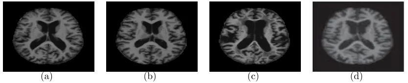
Figure 1.1 Sample Brain MRI Images from ADNI Database Presenting Different

Stages of Alzheimer’s Disease. (a) Normal/healthy controls (CN); (b)

Mild Cognitive Impairment(MCI); (c) Alzheimers Disease (AD). . 3

Figure 2.1 Relation Among AI, Machine Learning, and Deep Learning. . . . 12

Figure 2.2 Block Diagram of a Neural Network. . . 12

Figure 2.3 Illustration of a Convolutional Neural Network. . . 14

Figure 2.4 Local Connectivity of CNN. . . 15

Figure 2.5 Feature Map. . . 16

Figure 2.6 Max-Pooling Operation. Each Max is Taken Over 4 Numbers Ar-ranged in 2x2 Square. . . 17

Figure 2.7 The Major Components of A Magnetic Resonance Imaging System [1]. . . . 18

Figure 2.8 T1 and T2 Weighted Images of Brain [2]. . . 19

Figure 2.9 Structural MRI Images Presenting (a) Normal Control; (b) MCI; (c) AD. . . 20

Figure 2.10 Positron Emission Tomography (PET) Scanning Procedure [3]. . . 21

Figure 2.11 Example of Brain PET Images (a) Normal Control (b) MCI (c) AD. 22 Figure 4.1 Example of Different Brain MRI Images Presenting Different AD Stage. (a) Nondemented; (b) very mild dementia ; (c) mild dementia; (d) moderate dementia. . . 30

Figure 4.2 Block Diagram of Proposed Alzheimer’s Disease Detection and Clas-sification Framework. . . 31

Figure 4.3 Sample Images From OASIS Dataset. . . 33

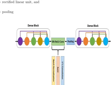
Figure 5.1 Illustration of Dense Connectivity with a 5-layer Dense Block. . . 39

(17)

Figure 5.3 Block Diagram of Proposed Alzheimer’s Disease Diagnosis

Frame-work. . . 40

Figure 5.4 Block Diagram of Individual Model M4. . . 45

Figure 5.5 Block Diagram of Individual Model M5. . . 46

Figure 5.6 Performance Comparison of the Proposed Model and the Variants. 49 Figure 5.7 Performance Comparison of the Proposed Model and the Baseline Deep CNNs. . . 50

Figure 5.8 Comparison of Accuracy on the OASIS Dataset. . . 50

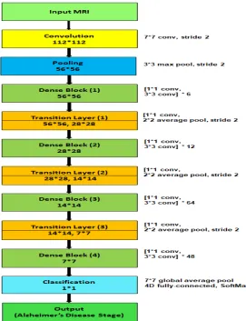
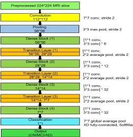
Figure 6.1 3D Brain MRI Preprocessing module. . . 54

Figure 6.2 Skull-Stripped MRI Slices Presenting Different AD Stages. (a)-(c) CN; (d)-(f) MCI; (g)-(i) AD. . . 55

Figure 6.3 Block Diagram of the Proposed Alzheimer’s Disease Diagnosis Frame-work. . . 55

Figure 6.4 Deep CNN Architecture Used for the Proposed Alzheimer’s Disease Diagnosis Framework. . . 56

Figure 7.1 Example of Brain PET images (a) Sagittal View (b) Coronal View (c) Axial View. . . 61

Figure 7.2 Proposed Synthetic Brain PET Image Generator. . . 62

Figure 7.3 Generator Architecture of the Proposed Model. . . 63

Figure 7.4 Discriminator Architecture of the Proposed Model. . . 64

Figure 7.5 Visualization of the Generator Output in the Training Process. . . 65

Figure 7.6 Real and Synthetic Brain PET Images of Normal Patient (a) Real (b) Synthetic. . . 66

Figure 7.7 Real and Synthetic Brain PET Images of MCI Patient (a) Real (b) Synthetic. . . 67

(18)

Figure 7.9 2D-Histograms of the Synthetic and Real Images. Top Row:

2D-Histogram of Real images. Bottom Row: 2D-2D-Histogram of Synthetic

Images. . . 70

Figure 8.1 Example of Brain PET Images (a) Normal Control (b) Mild Cognititve

Impairment (c) Alzheimer’s Disease. . . 74

Figure 8.2 Skull-Stripped PET Slices. . . 75

Figure 8.3 Alzheimer’s Disease diagnosis framework using PET data. . . 76

Figure 8.4 3D CNN Classifier for Alzheimer’s Disease and Mild Cognitive

Impair-ment diagnosis using PET data. . . 77

Figure 8.5 Relevance Heatmaps for Sensitivity Analysis (Backpropagation) Method

Averaged Over CN Patients. . . 78

Averaged Over MCI Patients. . . 80

Averaged Over AD Patients. . . 83

Figure 8.8 Relevance Heatmaps for Guided Backpropagation Method Averaged

Over CN Patients. . . 84

Over MCI Patients. . . 85

Over AD Patients. . . 86

Figure 8.11 Relevance Heatmaps for Occlusion Method Averaged Over CN

Pa-tients. . . 87

Figure 8.12 Relevance Heatmaps for Occlusion Method Averaged Over MCI

Pa-tients. . . 87

Figure 8.13 Relevance Heatmaps for Occlusion Method Averaged Over AD

(19)

Figure 8.14 Relevance Heatmaps for Brain Area Occlusion Method Averaged Over

CN Patients. . . 89

MCI Patients. . . 90

AD Patients. . . 91

Figure 8.17 Relevance Heatmaps for Layer-wise Relevance Propagation (LRP)

Method Averaged Over CN Patients. . . 92

Method Averaged Over MCI Patients. . . 93

Method Averaged Over AD Patients. . . 94

Figure 8.20 Visualization Comparison of the Relevance Heatmaps. (a) Sensitivity

Analysis ( Backpropagation). (b) Guided Backpropagation. (c)

Occlu-sion. (d) Brain Area OccluOcclu-sion. (e) Layer-wise Relevance Propagation

(20)

LIST OF ABBREVIATIONS

• GSU - Georgia State University

• CS - Computer Science

• AI - Artificial Intelligence

• ML - Machine Learning

• DL - Deep Learning

• NN - Neural Network

• CNN - Convolutional Neural Network

• MRI - Magnetic Resonance Imaging

• sMRI - Structural Magnetic Resonance Imaging

• AD - Alzheimer’s Disease

• MCI - Mild Cognitive Impairment

• CN - Normal Control

• CAD - Computer Aided Diagnosis

• ReLU - Rectified Linear Unit

• 3D - Three Dimensional

• RF - Radio–frequency

• TR - Repetition Time

(21)

• GM - Gray Matter

• WM - White Matter

• CSF - Cerebrospinal Fluid

• fMRI - Functional Magnetic Resonance Imaging

• PET - Position Emission Tomography

• SPECT - Single Photon Emission Computed Tomography

• DTI - Diffusion Tensor Imaging

• CT - Computed Tomography

• ROI - Region of Interest

• SVM - Support Vector Machine

• GLCM - Gray–Level Co-occurrence Matrix

• HC - Healthy Control

• PCA - Principal Component Analysis

• GAN - Generative Adversarial Network

• LRP - Layer-wise Relevance Propagation

(22)

Chapter 1

INTRODUCTION

In this chapter, we present the general introduction to this thesis intended to allow a

quick appraisal of its contents, contributions, supporting publications and structure.

1.1 AI-Assisted Disease Diagnosis

Artificial Intelligence (AI) has made substantial progress in recent days. AI is the area of

computer science that aims to mimic human cognitive functions and emphasize the creation

of intelligent machines. Today AI assisted models are performing incredible tasks with high

accuracy at a massive scale. AI has enabled us to build tools that can learn from experience,

adjust to new inputs and complete tasks with expert human-level performance. In this thesis,

we aim to use AI for solving various problems in the field of medical image analysis focusing

on improving performance for disease diagnosis.

Computer-aided diagnosis (CAD) refers to systems that provide information about

dis-ease assessment by interpreting medical images. AI can improve the performance of CAD

systems with discoveries and judgments leading to faster and more accurate diagnosis. AI

can handle a vast amount of information faster than any human with more accurate analysis.

Besides, AI can improve the accuracy by learning itself and acquiring expertise comparable

to specialists.

1.2 Medical Image Analysis

Medical image analysis focuses on extracting insights from images of biological tissue

with computational analysis. Medical Imaging creates visual representations of body

inte-rior for clinical assessment and uses several imaging techniques such as Computer

(23)

emission tomography (PET) etc. The scope of medical image analysis ranges from clinical

studies of medical imaging and disease in patients to neuroscience studies that target to find

scientific information such as human brain structure and functionality. Several

computa-tional methods such as signal processing, machine learning, biophysics etc. are used to built

applications for medical image analysis. In recent days deep learning techniques are helping

to identify, classify and qualify patterns in medical images with the advantages of learning

hierarchical feature representations directly from data instead of using hand-crafted features.

1.3 Classification in Medical Imaging

Image classification aims to assign an image to categories or classes of interest by

ana-lyzing its contents. In computer-aided diagnosis, image classification plays a significant role.

Classification in medical imaging refers to the task of analyzing an input image data and

assign it an output class indicating the presence of a disease or not. For example, classifying

patients as having Alzheimer’s Disease based on 3D brain MRI data.

1.3.1 Alzheimer’s Disease Diagnosis

Alzheimer’s Disease (AD) is the most prevailing type of dementia. The prevalence of

AD is estimated to be around 5% after 65 years old and is staggering 30% for more than

85 years old in developed countries. It is estimated that by 2050, around 0.64 Billion

peo-ple will be diagnosed with AD [4]. Alzheimer’s Disease destroys brain cells causing peopeo-ple

to lose their memory, mental functions and ability to continue daily activities. Initially,

Alzheimer’s Disease affects the part of the brain that controls language and memory. As a

result, AD patients suffer from memory loss, confusion, and difficulty in speaking, reading

or writing. They often forget about their life and may not recognize their family members.

They struggle to perform daily activities such as brushing hair or combing tooth. All these

make AD patients anxious or aggressive or to wander away from home. Ultimately, AD

(24)

There are three major stages in Alzheimer’s Disease - very mild, mild and moderate.

Detection of Alzheimer’s Disease (AD) is still not accurate until a patient reaches

mod-erate AD stage. For proper medical assessment of AD, several things are needed such as

physical and neurobiological exams, Mini-Mental State Examination (MMSE), and patient’s

detailed history. As AD is incurable, earlier diagnosis of AD can help for proper treatment.

For our research, we consider the automated diagnosis of Alzheimer’s Disease in 3D

struc-tural MRI brain scans and Positron Emission Tomography (PET) brain scans. We conduct

experiments using OASIS dataset and Alzheimer’s Disease Neuroimaging Initiative (ADNI)

dataset for classification of the Alzheimer’s Disease (AD), Mild Cognitive Impairment (MCI)

and CN (normal/healthy controls) to evaluate the proposed model. Mild Cognitive

Impair-ment (MCI) combines the very mild and mild stages of Alzheimer’s disease. Fig. 1.1 shows

some brain MRI images with different AD stages. As the disease progresses, Abnormal

pro-(a)

(b)

(c)

[image:24.612.168.463.381.644.2]

(25)

teins (amyloid-β [Aβ] and hyperphosphorylated tau) are accumulated in the brain of an AD

patient. This abnormal protein accumulation leads to progressive synaptic, neuronal and

axonal damage. The changes in the brain due to AD have a stereotypical pattern of early

medial temporal lobe (entorhinal cortex and hippocampus) involvement, followed by

pro-gressive neocortical damage [5]. Such changes occur years before the AD symptoms appear.

It looks like the toxic effects of hyperphosphorylated tau and/or amyloid-β [Aβ] gradually

erodes the brain, and when a clinical threshold is surpassed, amnestic symptoms start to

develop. Structural MRI (sMRI) and Positron Emission Tomography (PET) can be used

for measuring these progressive changes in the brain due to the AD. Our research work

fo-cuses on analyzing sMRI and PET data using deep learning model for Alzheimer’s Disease

diagnosis.

1.4 Feature Learning

Feature learning or representation learning refers to a set of methods that allows a model

to automatically identify the representations needed for feature detection or classification

from raw data. Feature learning aims to find an appropriate representation of data to

perform a machine learning task, eliminates the need to manual feature engineering and

allows a machine to learn the features themselves. Real world data - images and video

are complex and highly variable. For intelligent machines, it is necessary that they can

discover useful features or representations from the raw data themselves. Traditional

hand-crafted feature generation is expensive regarding time, cost and requires expert knowledge

and human labor. Moreover, they do not generalize well. Efficient feature learning techniques

can solve these issues and automate and generalize the learning process. Feature learning

algorithms have two categories: supervised and unsupervised feature learning. In Supervised

feature learning, the algorithm learns the feature from a labelled training dataset. On the

(26)

1.5 Deep Learning

Deep Learning is an area of Artificial Intelligence, specifically a part of Machine Learning

Algorithms. Recently, deep learning models have been famous for their ability to learn

fea-ture representations from the input data. Deep learning networks use a layered, hierarchical

structure to learn increasingly abstract feature representations from the data. Deep

learn-ing architectures learn simple, low-level features from the data and build complex high-level

features in a hierarchy fashion. Deep learning technologies have demonstrated revolutionary

performance in several areas, e.g., visual object recognition, human action recognition,

nat-ural language processing, object tracking, image restoration, denoising, segmentation tasks,

audio classification, brain-computer interaction, etc. Nowadays deep learning techniques are

being successfully applied for medical image analysis.

1.6 Objective

We developed computer-aided diagnosis models using deep learning technologies. We

explored a significant area in medical image analysis - classification. For classification task as

a case study, we developed automated models for Alzheimer’s disease diagnosis using brain

MRI and PET data. We worked for solving the class-imbalance problem in medical data and

developing efficient diagnosis models with limited training data. We propose solution to solve

limited dataset problem by generating synthetic medical images. We present approaches to

understand the decision of convolutional neural network to discriminate among samples of

different disease class.

1.7 Motivation

AI can offer several advantages over traditional analytics, and clinical decision-making

approaches. The health-care industry is a high priority sector where people expect the

highest level of service. Proper diagnosis of disease is crucial to treatment and saving a

(27)

an early stage, physicians can at least try to delay the harmful impact of the disease. On

the other hand, diagnosis is expensive and requires specialized expertise. In many countries

of the world, primary medical care is limited, and expert physicians are not available in time

of need. If we can build computer-aided-diagnosis systems that can automatically analyze

medical images and diagnosis disease with human-level expertise, it will reduce the cost of

treatment dramatically. Early diagnosis of disease will save the lives of millions of people

and bring exciting break-throughs in patient care.

While several research works have been done for analyzing natural images such as object

classification, recognition, tracking, segmentation etc., research in medical image analysis is

still limited. To mitigate the gap, we choose to focus on medical image analysis for developing

better disease diagnosis systems.

1.8 Challenges

For our research, we plan to use deep learning technologies for medical image analysis.

There are several challenges related to working with medical data. First, medical images

are generally private and having access to those data is challenging and often impossible.

Second, for natural image analysis such as object classification, millions of data are available

to train an automated classifier. On the other hand, in disease classification, typically

few hundreds data sample are available. Third, it requires specialized expertise to capture

and annotate the ground truth data for the learning process. Often availability of those

experts is limited. Fourth, the dataset is often imbalanced. When we develop an automated

disease diagnosis model, we require enough sample data from both the positive and negative

class. In medical image analysis, typically more than 90% data belongs to the positive class.

Additionally, there are heterogeneous image data available due to different image capturing

protocol. Several pre-processing steps are necessary so that the algorithm can work with

varying types of data.

Deep Learning models learn automatically from the input data without requiring any

(28)

model that has achieved tremendous success in image analysis task. In our research work,

we are going to use CNN for developing the automated diagnosis model. CNN requires a

vast training dataset for efficient training. But in medical image analysis, such large dataset

is not available. Designing an efficient classifier that can work with limited training data is

a significant challenge in medical image analysis.

Analyzing medical images requires significant expertise. As we are working for

Alzheimer’s Disease Diagnosis, we have seen that there is a similarity in the normal healthy

brain data of older people and the Alzheimer’s Disease data. It is very challenging to

dif-ferentiate between both. Diagnosing AD at an early stage is even more challenging, and

extensive knowledge and experience are required.

1.9 Contribution

The current thesis presents a multidisciplinary research efforts to investigate the

emerg-ing deep learnemerg-ing technologies for medical image analysis. We have developed several models

for Alzheimer’s disease diagnosis using deep learning technologies that outperform previous

state-of-the-art. We have presented preprocessing approaches for better analysis of MRI

data. We have demonstrated approaches that can solve the class-imbalance problem in

medical image analysis. We have experimented and introduced several ways to improve

the performance of a CNN classifier for disease diagnosis with limited training data. We

proposed solution to solve limited dataset problem by generating synthetic medical images

and presented approaches to understand the decision of convolutional neural network to

(29)

1.10 List of Publications

• Islam, J., Zhang, Y.: Visual sentiment analysis for social images using transfer learning

approach. In: 2016 IEEE International Conferences on Big Data and Cloud Computing

(BDCloud), Social Computing and Networking (SocialCom), Sustainable Computing

and Communications (SustainCom) (BDCloud-SocialCom-SustainCom), pp. 124–130.

IEEE (2016).

• Islam, J., Zhang, Y.: A novel deep learning based multi-class classification method for

Alzheimers Disease detection using brain MRI data. In: Zeng, Y., et al. (eds.) BI

2017. LNCS, vol. 10654, pp. 213–222. Springer, Cham (2017).

• Islam, J., Zhang, Y.: An ensemble of deep convolutional neural networks for Alzheimers

disease detection and classification. arXiv preprint arXiv:1712.01675 (2017).

• Islam, J., Zhang, Y.: Brain MRI analysis for Alzheimers disease diagnosis using an

ensemble system of deep convolutional neural networks. Brain Informatics. 5(2), 2

(2018).

• Islam, J., Zhang, Y.: Early diagnosis of Alzheimers disease: a neuroimaging study with

deep learning architectures. In: Proceedings of the IEEE Conference on Computer

Vision and Pattern Recognition Workshops, pp. 18811883 (2018).

• Islam, J., Zhang, Y.: Deep Convolutional Neural Networks for Automated Diagnosis of

Alzheimers Disease and Mild Cognitive Impairment Using 3D Brain MRI. In: Shouyi,

W., et al. (eds.) BI 2018. LNCS, vol. 11309, pp. 359–369. Springer, Cham (2018).

• Islam, J., Zhang, Y.: Towards Robust Lung Segmentation in Chest Radiographs with

Deep Learning. arXiv preprint arXiv:1811.12638 (2018).

Submitted manuscripts

• Islam, J., Zhang, Y.: A Robust EEG-based Brain-Machine Interface for Mental

(30)

• Islam, J., Zhang, Y.: GAN-based Synthetic Brain PET Image Generation. (Under

Review, 2019)

• Islam, J., Zhang, Y.: Understanding Behavior of 3D Convolutional Neural Network

for Alzheimer’s Disease and Mild Cognitive Impairment Diagnosis Using PET Data.

(31)

1.11 Thesis Outline

The remainder of this thesis is organized as follows. Chapter 2 presents background

study related to deep learning and medical image analysis. Chapter 3 reviews existing

approaches to Alzheimer’s Disease Diagnosis and Lung segmentation. Chapter 4, 5, and 6

present our proposed approaches for Alzheimer’s Disease diagnosis. Chapter 7 presents our

proposed approach to generate synthetic medical images. Chapter 8 describes our method

for understanding behavior of 3D Convolutional Neural Network for Alzheimer’s Disease and

Mild Cognitive Impairment diagnosis. Finally, Chapter 9 presents the directions for future

(32)

Chapter 2

BACKGROUND STUDY

In this chapter, we discuss an overview of some background ideas of the ensuing sections

of this thesis. To set the stage, we review feature learning algorithms and neural network

models. Next, we discuss in detail about Convolutional Neural Network (CNN) which is

the underlying architecture of the proposed diagnosis frameworks of this thesis. We briefly

describe Generative Adversarial Networks that were used to generate synthetic medical

im-ages. Finally, we present the theory behind Magnetic Resonance Imaging (MRI), Structural

MRI (sMRI) analysis, Positron Emission Tomography (PET), and PET analysis.

Artificial Intelligence (AI) is an area of computer science that focuses on the creation

of intelligent machines. AI algorithms simulate intelligent behaviour in computers that

can work and behave like a human. Machine Learning is a group of AI techniques that

use statistical methods to enable machines to learn with data, without being explicitly

programmed and improve with experiences. Deep Learning is a subset of machine learning

as shown in Figure 2.1. Deep Learning models solve problems by using neural networks ( a

series of algorithms modelled after the human brain).

2.1 Learning Algorithms

Machine Learning models are divided into two broad categories - supervised and

unsu-pervised algorithms. In suunsu-pervised learning, there is input data (X) and output variable (Y)

and the algorithm learns the mapping function from input to output.

f :X →Y; (2.1)

Y typically represents an instance from a fixed set of class. The target of the learning

(33)

Figure (2.1) Relation Among AI, Machine Learning, and Deep Learning.

comes, the model can predict the output class for it. For example, an algorithm trained on

the labelled dataset of benign or malignant tumours learns to identify patients with cancer

or not.

On the contrary, unsupervised algorithms learn to process data without any label and

can identify patterns without any guidance. For example, clustering algorithms can discover

the inherent groupings in the data, such as grouping customers by purchasing behaviour.

(34)

2.2 Neural Network

Neural networks or Artificial neural networks are a set of learning algorithms that

replicate the way humans learn. They consist of connected neurons or learning units with

some activation function a and parameters Θ = {ω, β}, where ω is a set of weights and β

is a set of biases. Neural networks are organized in layers consisted of neurons. Input data

is passed to the network via the ‘input layer’, which communicates to one or more ‘hidden

layers’ where the actual processing is done. The hidden layers transform the input and then

link to an ’output layer’ that produces the output. Figure 2.2 shows block diagram of a basic

neural network. The activation function is a linear combination of the input to the neurons

and the parameters:

a=σ(ωTx+b) (2.2)

Deep learning methods often use neural networks with lots of hidden layers and are

often referred to as deep neural networks.

2.3 Convolutional Neural Network

Convolutional neural network (CNN) is a feed-forward artificial neural network and

the most popular deep learning model. Artificial neural networks are systems of connected

neurons that exchange messages with each other. The connections have respective weights

that can be tuned based on experience. As a result, neural networks become adaptive to

inputs and capable of learning. Since regular neural networks have fully connected neurons,

so they do not scale well to full images. If an image is of size 28x28x3, a single fully connected

neuron in the first hidden layer will have 28*28*3 = 2352 weights. Now if the image is of

size 512x512x3, the weight would be 512*512*3 = 786,432 for a single neuron. Now it is very

much expected that the full network will have a lot of neurons. As a result, the parameters

will add up quickly too. So not only the full connectivity would be wasteful, but also the

high number of parameters would lead to overfitting.

(35)

nodes to the output nodes via the hidden nodes (if any). CNN assumes that inputs are images

and thus encodes specific properties to the architecture. As a result, the forward function

becomes more efficient, and the amount of parameters in the network reduces vastly too.

In a convolutional neural network, the neurons are arranged in three dimensions - weight,

height, and depth. So if the input image has size 28x28x3, then the input volume would have

dimension 28x28x3. A small region of the layer would be connected to the neurons of the

next layer. They won’t be connected fully to all neurons in the next layer. The input image

would be reduced to a single vector of class scores by the final output layer. The vector would

be arranged along the depth dimension. Each layer converts the 3D input volume to a 3D

output volume of neuron activations. The depth of the layer is equal to the number of color

channels in the image. Width and heights are determined by the dimension of the image.

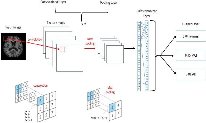
Each layer of a CNN uses a differentiable function to convert one volume of activations to

Figure (2.3) Illustration of a Convolutional Neural Network.

another. There are three main types of layers - Convolutional Layer, Pooling Layer, and

Fully-Connected Layer. These layers are stacked to form a full CNN architecture. The

neurons connected to the local regions of the input computes a dot product of their weights

[image:35.612.126.484.362.575.2]

(36)

layer performs a downsampling operation along the spatial dimensions - width and height.

The fully connected layer where each neuron is connected to all the numbers of the previous

volume computes the output class score. Thus, an input image is converted to a final class

score by layer by layer transformation of the original pixels. The convolutional and fully

connected layer has parameters such as weights and biases of neurons. The transformation of

these layers is a function of the activations of the input volume and these parameters. These

parameters are trained with gradient descent in such a way so that the output class score is

consistent with each training image. The pooling layers have fixed functions. There are two

other layers - ReLU layer and Loss layer. ReLU layer increases the nonlinear properties of

the decision function. Loss layer uses different loss functions for different tasks. For example,

to predict a single class of K mutually exclusive classes, Softmax loss is used.

Figure (2.4) Local Connectivity of CNN.

2.3.1 Local Connectivity

CNN enforces a local connectivity pattern between adjacent layer neurons and thus

utilizes spatially-local correlation. Figure 2.4 shows local connectivity in a CNN. Here the

inputs of hidden units of layer m are generated from a subset of units of layer m-1. The units

of layer m-1 have spatially adjacent receptive fields. Let us consider layer m-1 as input. Layer

m units are connected to 3 adjacent neurons in the layer. So we can say that the receptive

field width of layer m is 3. Receptive field width of layer m+1 is also 3 concerning layer m.

But with respect to the input layer, the receptive field width of layer m+1 is 5. Each unit

does not respond to variations outside of its receptive field with respect to the input layer.

(37)

local input pattern. Now if we stack multiple layers, then the filters would become global

gradually and response to a larger region of pixel space. As in the figure, we can see neurons

of hidden layer m+1 can encode a feature of width 5.

Figure (2.5) Feature Map.

2.3.2 Shared Weights

One crucial feature of CNN is each filter hi is replicated across the entire visual field.

Same weight and bias are shared by these replicated units, and a feature map is produced. By

sharing the same weights, CNN achieves shift-invariant property. So CNN can detect features

regardless of their position. Sharing weight thus allows CNN to achieve high performance

in recognition and detection problem. The need to learn free parameters is also decreased

significantly, so learning efficiency improves. It also reduces the required memory size. Figure

2.5 shows a feature map consisted of 3 units. We obtain a feature map by repeatedly applying

a function across the sub-regions of the input image that is the convolution of the image with

a linear filter and adding a bias term and applying a non-linear function,σ. The k–th feature

map at a given layer can be denoted as hk_{. If the filters of feature map h}k _{is determined by}

weights Wk and bias bk, then we can write:

hk_ij =σ((Wk∗x)ij +bk) (2.3)

2.3.3 Pooling

Pooling operation reduces the spatial size of the data representation and helps to reduce

(38)

two popular pooling operations. Max pooling is also known as down-sampling. The input

image is partitioned into a set of non-overlapping rectangles. Then for each sub-region, the

maximum value is computed. Since non-maximal values are eliminated, so computation for

upper layers are reduced. Max pooling also provides translation invariance. If we cascade a

max-pooling layer with a convolutional layer, we get eight directions to translate the input

image by a single pixel. Now if max-pooling is done in a 2x2 region, out of the eight possible

configurations, three will provide the same output at the convolutional layer. If the region

size is 3x3, 5 out of 8 regions will give the same output. Because of this robustness,

max-pooling is used to reduce the dimension of intermediate representations. Figure 2.6 presents

an example of max–pooling operation.

Figure (2.6) Max-Pooling Operation. Each Max is Taken Over 4 Numbers Arranged in 2x2 Square.

2.4 Generative Adversarial Networks

Generative Adversarial Networks (GANs) is a deep learning architecture that consisted

of two models - a generative model G and a discriminative model D. The generative model

captures the data distribution. The discriminative model estimates the probability that the

sample is drawn from the training data rather than the generative model. The two models

are simultaneously trained via an adversarial process. The architecture is inspired by game

theory and corresponds to a minimax two-player game. The training procedure of G is to

maximize the probability of D making a mistake [6].

(39)

percep-tron with parametersθg that depicts a mapping to the data space. To learn the generator’s

distribution ρg over the data space x, a prior ρz is defined on random input noise variables

z. The discriminator D (x, θd) is also a neural network that gets a sample the real dataset

or the generated synthetic dataset produced by G and outputs a single scalar value that

the input data comes from the real training dataset. The training process focuses on the

task that the discriminator D will maximize the probability of assigning correct labels to the

training examples and generated samples from G. At the same time, G is trained to generate

data samples similar to the real dataset so that D cannot differentiate them from actual

data. Similar to game theory, the discriminator D and the generator G play a two-player

mini-max game with following value function V(G, D):

min

G maxD V(D, G) = Ex∼ρdata(x)[logD(x)] +Ez∼ρdata(z)[log(1−D(z))] (2.4)

Where xis the real data andz is the input random noise. ρdata,ρz represent the

distri-bution of the real data and the input noise. D(x) represents the probability thatxcame from

the real data while G(z) represents the mapping to synthesize the real data. The generator,

G is a deeper neural network and have more convolutional layers and nonlinearities. The

noise vector z is upsampled while G learns the weights through backpropagation. At some

point, the generator starts producing data that is classified as real by the discriminator.

(40)

2.5 Magnetic Resonance Imaging

Magnetic Resonance Imaging (MRI) is a technique that creates a 3D representation of

body structures using magnetic fields and radio waves. Nowadays it is a standard practice

to use MRI to detect changes in the body caused by different diseases. Magnetic Resonance

Imaging was developed around 1980. MRI is a powerful imaging technique to visualizing

detailed structures in vivo. MRI technique uses magnetic manipulation of protons to acquire

images without ionizing radiation. In the MRI scanner, the patient is placed in a strong

mag-netic field that causes the hydrogen atoms (protons in the water molecules) in the patients

body to align either in parallel or anti-parallel to the magnetic field.

Figure 2.7 shows the major components of a Magnetic Resonance Imaging system.

Protons are randomly oriented within the water nuclei of the tissue.Radio-frequency (RF)

pulses emitted from the radio-frequency coils in the MRI system causes the proton to spin

on its axis. When the RF pulse is turned off, protons return to their resting alignment and

emit RF energy. The emitted signals are measured after a certain period following the initial

RF to produce the Three Dimensional (3D) grey-scale image. Proton spin relaxation rate

differs depending on their tissue type and decides the intensity level of the image. Different

types of images are created using a different sequence of RF pulses. Repetition Time (TR)

refers to the amount of time between consecutive pulse sequences applied to the same slice.

Time to Echo (TE) indicates the time between the transmission of the RF pulse and the

receipt of the echo signal [1].

(41)

T1 and T2 are two commonly used relaxation times for protons. T1 or longitudinal

relaxation time is the measure of time taken for spinning protons to realign with the external

magnetic field. It determines the rate at which excited protons return to equilibrium. T2

or transverse relaxation time is the measure of the time taken for spinning protons to lose

phase coherence among the nuclei spinning perpendicular to the main field. It determines

the rate at which excited protons reach equilibrium or go out of phase with each other [2].

Figure 2.8 shows T1 and T2 weighted images of brain. T1-Weighted MRI is produced with

short TE and short TR (TR<1000 ms, TE<30 ms ) while long TE and long TR (TR>2000

ms, TE >80 ms) is used to obtain T2-weighted images. In a T1-weighted brain MRI, the

Gray Matter (GM) is visible as a dark grey area, the White Matter (WM) is light grey, and

the Cerebrospinal Fluid (CSF) is black. On the other hand, in T2-weighted brain images,

GM is light grey, WM is dark grey, and CSF is bright.

(a) (b) (c)

Figure (2.9) Structural MRI Images Presenting (a) Normal Control; (b) MCI; (c) AD.

2.5.1 Structural MRI (sMRI)

Structural magnetic resonance imaging (sMRI) is used to examine the physical structure

of the brain. It translates the differences in the water content with different shades of grey

(42)

tissue contrast that helps to identify changes in the brain such as the presence of tumours.

For our research, we analyze sMRI for Alzheimer’s Disease diagnosis. Figure 2.9 shows

structural MRI images presenting different stages of Alzheimer’s Disease.

2.6 Positron Emission Tomography (PET)

Positron Emission Tomography is a class of nuclear medicine imaging. It is also known

as PET imaging or a PET scan. Nuclear medicine refers to a type of medical imaging

meth-ods that utilizes radioactive material in a small amount to diagnose and determine the stage

of a disease or treat a disease. Nuclear Medicine procedures are known for their ability to

pinpoint molecular activity within the body. So, they have the potential to diagnose the

disease in the earliest stage and find patient’s response to therapeutic interventions. These

procedures are used to diagnose different types of cancers, heart disease, gastrointestinal,

endocrine, neurological disorders and other abnormalities within the body. Radioactive

ma-terials known as radiopharmaceuticals or radiotracers are used to perform nuclear medicine

imaging procedures.

Positron Emission Tomography (PET) uses small amounts of radiotracers, a special

cam-Figure (2.10) Positron Emission Tomography (PET) Scanning Procedure [3].

(43)

(PET) measures the body changes at the cellular level by looking at blood flow, metabolism,

neurotransmitters, and radiolabelled drugs. PET may identify early onset of disease before

it is evident on other imaging tests. It performs quantitative analyses and finds relative

changes over time as the disease process evolves or in response to a specific stimulus [3].

Figure 2.10 presents the procedure to perform PET scan. Depending on the organ or tissue

to study, the tracer can be injected, swallowed or inhaled. A small amount of a radioactive

tracer is administered into a peripheral vein, and the radioactivity emitted is measured. The

tracer is injected as an intravenous injection usually labelled with oxygen-15, fluorine-18,

carbon-11, or nitrogen-13. The areas of the disease often demonstrate higher levels of

chem-ical activity and the tracer collects in areas of your body. On the PET scan, these areas

might show up as bright spots. The total radioactive dose is similar to the dose used in

Computed Tomography (CT).

(a) (b) (c)

Figure (2.11) Example of Brain PET Images (a) Normal Control (b) MCI (c) AD.

PET imaging tracers can correlate β-amyloid deposition in the brain. The amyloid

deposition in the brain can be detected years before the onset of clinical signs of Alzheimer’s

Disease. The PET imaging tracers can help in differentiating dementia syndromes at the

early stage. PET scans reflect the resting state cerebral metabolic rates of glucose that is an

indicator of neuronal activity. Cerebral glucose metabolic alterations have distinct patterns

that can be used to identify Alzheimer’s Disease symptoms. Fig. 2.11 shows some brain PET

(44)

(45)

Chapter 3

REVIEW OF THE STATE-OF-THE-ART

In this section, we review the related work focusing on Alzheimer’s Disease Diagnosis,

synthetic medical image generation and CNN Visualization.

3.1 Alzheimer’s Disease Diagnosis

Detection of physical changes in brain complement clinical assessments and has an

increasingly important role for early detection of AD. Researchers have been devoting

their efforts to Neuroimaging techniques to measure pathological brain changes related to

Alzheimer’s disease. Machine learning techniques have been developed to build classifiers

using imaging data and clinical measures for AD diagnosis [7], [8], [9], [10], [11], [12], [13],

[14], [15], [16]. These studies have identified the significant structural differences in the

re-gions such as the hippocampus and entorhinal cortex between the healthy brain and brain

with AD. Changes in cerebrospinal tissues can explain the variations in the behavior of the

AD patients [17], [18]. Besides, there is a significant connection between the changes in brain

tissues connectivity and behavior of AD patient [19]. The changes causing AD due to the

degeneration of brain cells are noticeable on images from different imaging modalities, e.g.,

structural and functional Magnetic Resonance Imaging (sMRI, fMRI), Position Emission

To-mography (PET), Single Photon Emission Computed ToTo-mography (SPECT), and Diffusion

Tensor Imaging (DTI) scans. Several researchers have used these neuroimaging techniques

for AD Diagnosis. For example, sMRI ([20], [21], [22], [23], [24], [25]), fMRI([26], [27]), PET

([28], [29]), SPECT ([30], [31], [32]), and DTI ([33], [34]) have been used for diagnosis or

prognosis of AD. Moreover, information from multiple modalities have been combined to

improve the diagnosis performance ([35], [36], [37], [38], [39], [40], [41], [42], [43], [44], [45],

(46)

A classic Magnetic Resonance Imaging (MRI) based automated AD diagnostic

sys-tem has mainly two building blocks - feature/biomarker extraction from the MRI data and

classifier based on those features/biomarkers. Though various types of feature extraction

techniques exist, there are three major categories - (1) voxel-based approach, (2) Region

of Interest (ROI)-based approach, and (3) patch-based approach. Voxel-based approaches

are independent of any hypothesis on brain structures [47], [48], [49], [50]. For example,

voxel-based morphometry measures local tissue (i.e., white matter, gray matter, and

cere-brospinal fluid) density of the brain. Voxel-based approaches exploit the voxel intensities as

the classification feature. The interpretation of the results are simple and intuitive in

voxel-based representations, but they suffer from the over-fitting problem. Since there are limited

(e.g., tens or hundreds) subjects with very high (millions) dimensional features [51], which

is a major challenge for AD diagnosis based on neuroimaging. To achieve more compact

and useful features, dimensionality reduction is essential. Moreover, voxel-based approaches

suffer from the ignorance of regional information.

Region of Interest (ROI)-based approach utilizes the structurally or functionally

pre-defined brain regions and extracts representative features from each region [21], [24], [27],

[28], [52], [53],[54]. These studies are based on specific hypothesis on abnormal regions of

the brain. For example, some studies have adopted gray matter volume [55], hippocampal

volume [56], [57], [58] and cortical thickness [21], [59]. ROI-based approaches are widely used

due to relatively low feature dimensionality and whole brain coverage. But in ROI-based

ap-proaches, the extracted features are coarse as they cannot represent small or subtle changes

related to brain diseases. The structural or functional changes that occur in the brain due

to neurological disorder are typically spread to multiple regions of the brain. As the

ab-normal areas can be part of a single ROI or can span over multiple ROIs, voxel-based or

ROI-based approaches may not efficiently capture the disease-related pathologies. Besides,

the Region of Interest (ROI) definition requires expert human knowledge. Patch-based

ap-proaches [20], [60], [61], [62], [63], [64], [65] divide the whole brain image into small-sized

(47)

identification, so the necessity of human expert involvement is reduced compared to

ROI-based approaches. Compared to voxel-ROI-based approaches, patch-ROI-based methods can capture

the subtle brain changes with significantly reduced dimensionality. Patch-based approaches

learn from the whole brain and better captures the disease related pathologies that results

in superior diagnosis performance. However, there is still challenges to select informative

patches from the MRI images and generate discriminative features from those patches.

A large number of research works focused on developing advanced machine learning

models for AD diagnosis using MRI data. Support Vector Machine SVM), Logistic Regressors

(e.g., Lasso, and Elastic Net), Sparse Representation based Classification (SRC), Random

Forest Classifier, etc. are some widely used approaches. For example, Kloppel et al. [50]

used linear SVM to detect AD patients using T1 weighted MRI scan. Dimensional reduction

and variations methods were used by Aversen et al. [66] to analyze structural MRI data.

They have used both SVM binary classifier and multi-class classifier to detect AD from

MRI images. Vemuri et al. [67] used SVM to develop three separate classifiers with MRI,

demographic and genotype data to classify AD and healthy patients. Katherine Gray [68]

developed a multi-modal classification model using random forest classifier for AD diagnosis

from MRI and PET data. Amulya et al. [69] used Gray-Level Co-occurrence Matrix (GLCM)

method for AD classification. Morra et al. [70] compared several model’s performances

for AD detection including hierarchical AdaBoost, SVM with manual feature and SVM

with automated feature. For developing these classifiers, typically predefined features are

extracted from the MRI data. However, training a classifier independent from the feature

extraction process may result in sub-optimal performance due to the possible heterogeneous

nature of the classifier and features [71].

Recently, deep learning models have been famous for their ability to learn feature

repre-sentations from the input data. Deep learning networks use a layered, hierarchical structure

to learn increasingly abstract feature representations from the data. Deep learning

architec-tures learn simple, low-level feaarchitec-tures from the data and build complex high-level feaarchitec-tures in a

(48)

in several areas, e.g., visual object recognition, human action recognition, natural language

processing, object tracking, image restoration, denoising, segmentation tasks, audio

classi-fication, brain-computer interaction, etc. In recent years, deep learning models specially

Convolutional Neural Network (CNN) have demonstrated excellent performance in the field

of medical imaging, i.e., segmentation, detection, registration, and classification [72]. For

neuroimaging data, deep learning models can discover the latent or hidden representation

and efficiently capture the disease-related pathologies. So, recently researchers have started

using deep learning models for AD and other brain disease diagnosis.

Gupta et al. [64] have developed a sparse autoencoder model for AD, Mild Cognitive

Impairment (MCI) and healthy control (HC) classification. Payan et al. [65] trained sparse

autoencoders and 3D CNN model for AD diagnosis. They also developed a 2D CNN model

that demonstrated nearly identical performance. Brosch et al. [73] developed a deep belief

network model and used manifold learning for AD detection from MRI images. Hosseini-As

et al. [74] adapted a 3D CNN model for AD diagnostics. Liu et al. [75] developed a deep

learning model using both unsupervised and supervised techniques and classified AD and

MCI patients. Liu et al. [76] have developed a multimodal stacked auto-encoder network

using zero-masking strategy. Their target was to prevent loss of any information of the image

data. They have used SVM to classify the neuroimaging features obtained from MR/PET

data. Sarraf et al. [77] used fMRI data and deep LeNet model for AD detection. Suk et

al. [20], [41], [78], [79] developed an autoencoder network-based model for AD diagnosis

and used several complex SVM kernels for classification. They have extracted low to mid

level features from magnetic current imaging (MCI), MCI-converter structural MRI, PET

data and performed classification using multi-kernel SVM. C´ardenas-Pe˜na et al. [80] have

developed a deep learning model using central kernel alignment and compared the supervised

pre–training approach to two unsupervised initialization methods, autoencoders and

Princi-pal Component Analysis (PCA). Their experiment shows that SAE with PCA outperforms

three hidden layers SAE and achieves an increase of 16.2% in overall classification accuracy.

(49)

pro-gression of cognitive decline. No treatment can stop or reverse the propro-gression of AD. So,

early diagnosis of AD is essential for preventive and disease-modifying therapies. Most of

the existing research work on AD diagnosis focused on binary classification problems, i.e.,

differentiating AD patients from healthy older adults. However, for early diagnosis, we need

to distinguish among current AD stages, which makes it a multi-class classification problem.

In our initial work [81], we developed a very deep convolutional network and classified the

four different stages of the AD - nondemented, very mild dementia, mild dementia, and

moderate dementia. We improved the previous model, developed an ensemble of deep

con-volutional neural networks [82], and demonstrated better performance on the Open Access

Series of Imaging Studies (OASIS) dataset [83]. Additionally, we developed an efficient deep

convolutional neural network based classifier [84] and demonstrated better performance on

the ADNI dataset [85].

3.2 Medical Image Synthesis

Medical Image synthesis and Generative Adversarial networks have got attention in

re-cent years. Costa et al. [86] used a fully-convolutional neural network to train on retinal

vessel segmentation images and then applied GANs for generating synthetic retinal images.

Dai et al. [87] used GANs for creating lung fields and heart segmentation images from chest

X-ray images. Shin et al. [88] utilized GANs for generating synthetic abnormal MRI images

with brain tumors. Nie et al. [89], proposed an auto-context model for brain CT and MRI

image refinement. Schlegl et al. [90] trained GANs for anomaly detection in retinal images.

Frid-Adar et al. [91] applied GANs for synthesizing liver lesion ROIs to apply in liver lesion

classification. Hu et al. [92] applied GANs to generate a MRI motion model. Mahapatra

et al. [93] synthesized high-resolution retinal fundus images using generative adversarial

networks. Nie et al. [89] generated synthetic pelvic CT images using GANs.

In our previous research works, we had to handle the limited dataset problem for

(50)

for Alzheimer’s Disease diagnosis. Besides, there are very few works done for PET image

synthesis. To mitigate these gaps, we propose a novel model to generate synthetic brain

Positron Emission Tomography (PET) images exploiting Generative Adversarial Networks

for three stages of Alzheimer’s Disease - Normal Control (CN), Mild Cognitive Impairment

(MCI), and Alzheimer’s Disease (AD).

3.3 CNN Visualization

Recently, several visualization methods for CNN interpretation have been proposed.

Some of these methods focus on synthesizing the image that maximizes the score of a given

unit in a pretrained CNN, while others invert feature maps of a conv-layer back to the input

image. Among the gradient-based methods, deconvnet with Occlusion Sensitivity [94],

Sensi-tivity analysis with backpropagation [95], Guided Backpropagation (GB) [96] demonstrated

notable performance. These methods compute the gradients of the score of the convolutional

neural network with respect to the input image. The gradients that maximize the neuron

score are used to estimate the image appearance.

Rieke et al. [97] compared four visualization methods to understand a CNN behavior

for AD diagnosis using MRI data. B¨ohle et al. [98] presented an approach utilizing

Layer-wise Relevance Propagation (LRP) [99] for CNN visualization for AD diagnosis. Korolev et

al. [100] applied the occlusion method to interpret a deep CNN. They mainly focused on

developing a 3D-CNN classifier and didn’t employ different visualization method. Yang et

al. [11] presented segmentation-based occlusion approach to find visual explanations that

can indicate a 3D-CNNs spatial attention on MRI brain scans when making predictions. To

the best of our knowledge, our work is the first to understand CNN behavior for Alzheimer’s

(51)

Chapter 4

A NOVEL DEEP LEARNING BASED MULTI-CLASS CLASSIFICATION

METHOD FOR ALZHEIMER’S DISEASE DIAGNOSIS

4.1 Introduction

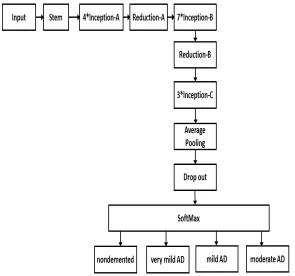
In this chapter, we describe our initial work and present a novel deep learning model

for multi-Class Alzheimer’s Disease detection and classification using Brain MRI Data. We

design a very deep convolutional network and demonstrate the performance on the Open

Access Series of Imaging Studies (OASIS) dataset [83]. Fig. 7.1 shows some brain MRI

images presenting different AD stage.

(a) (b) (c) (d)

Figure (4.1) Example of Different Brain MRI Images Presenting Different AD Stage. (a) Nondemented; (b) very mild dementia ; (c) mild dementia; (d) moderate dementia.

4.2 Method

In this section, the proposed Alzheimer’s disease detection and classification framework

would be presented. The proposed model is shown in Fig. 4.2. Our model is inspired by

Inception-V4 network [101]. After the preprocessing is done, the input is passed through

a stem layer. A stem layer includes several 3*3 convolution layers, 1*1 convolution layer,

[image:51.612.98.515.379.464.2]

(52)

and two expansion layers (1*1 convolution layer). Inception-A module has four

filter-expansion layers, three 3*3 convolution layer, and one average pooling layer. Inception-B

module has four filter-expansion layers, four 1*7 convolution layer, two 7*1 convolution layer

and one average pooling layer. Inception-C module has four filter-expansion layers, three 1*3

convolution layer, three 3*1 convolution layer and one average pooling layer. Reduction-A

module has one filter-expansion layer, three 3*3 convolution layer, and one 3*3 max-pooling

layer. The Reduction-B module has two filter-expansion layers, two 3*3 convolution layer,

one 1*7 convolution layer, one 7*1 convolution layer and one 3*3 max pooling layer. The

input and output of all these modules pass through filter concatenation process. We have

redesigned the final softmax layer for Alzheimer’s disease detection and classification. The

softmax layer has four different output class: nondemented, very mild, mild and moderate

AD. The network takes an MRI image as input and extracts layer-wise feature representation

from the first stem layer to the last drop-out layer. Based on this feature representation, the

input MRI image is classified to any of the four output classes.

[image:52.612.160.455.403.679.2]

(53)

To measure the loss of the proposed network, we have used cross entropy. The Softmax

layer takes the feature representation, fi and interprets it to the output class. A probability

score, pi is also assigned for the output class. If we define the number of Alzheimer’s disease

stages as m, then we get

pi =

exp(fi)

P

iexp(fi)

, i= 1, ..., m

and

L=−X

i

tilog(pi),

where L is the loss of cross entropy of the network. Back propagation is used to calculate

the gradients of the network. If the ground truth of an MRI image is denoted as ti, then,

∂L ∂fi

=pi−ti

There is numerous possible combination for the hyper-parameters of a network. It takes

a lot of time and effort to decide a stable hyperparameter set for a network. To reduce this

time, we have used hyperparameters of the Inception-V4 model [101] instead of random

initialization. The weights and biases of the inception-v4 model [101] pre-trained with

Ima-geNet database [102] provide our network an efficient hyperparameter set. As a result, the

model has a sense of better feature detector and can use that knowledge for learning features

from the small medical image dataset. We have trained our model with OASIS [83] dataset.

To prevent overfitting in the network, we have applied data augmentation technique such as

reflection and scaling.

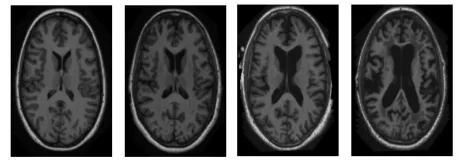
4.3 Data

OASIS dataset is prepared by Dr. Randy Buckner from the Howard Hughes Medical

Institute (HHMI) at Harvard University, the Neuroinformatics Research Group (NRG) at

Washington University School of Medicine, and the Biomedical Informatics Research

(54)

T1-weighted MRI scans are available. 100 of the patients having age over 60 are included in

the dataset with very mild to moderate AD. Fig. 4.3 shows some sample brain MRI images

from OASIS dataset.

Figure (4.3) Sample Images From OASIS Dataset.

4.4 Experiments

We have implemented the proposed deep CNN model for Alzheimer’s disease detection

and classification using Tensorflow [30] and Python on a Linux X86-64 machine with AMD A8

CPU, 16 GB RAM and NVIDIA GeForce GTX 770. We have applied data augmentations

techniques - scaling and reflection on the images. Since the dataset is small, 5-fold cross

validation is performed on the dataset. For each fold, We have used 70% as training data,

10% as validation data and 20% as test data. The input size of the Inception-V4 network

[101] is 299*299*3. To fit the MRI data, we have designed the input size of our network as

299*299*1. We have modified the Inception B and C module so that they can accept the

MRI data. The convolutional filter size of Inception-B is 1154 in the original network. We

made it to 1152 to fit the MRI data. The convolutional filter size of Inception-C is 2048 in

the original network. We made it to 2144 to fit the MRI data. The network is optimized

with the RMSProp [103] algorithm and early-stopping is used for regularization. The decay

[image:54.612.190.420.178.258.2]