Gross Worker Flows over the Business Cycle

Gross Worker Flows over the Business Cycle

November 2012

Abstract

We build a hybrid model of aggregate labor supply with predictions for gross flows across the three labor market states: employment, unemployment, and non-participation. We use this model to assess the role of labor supply over the business cycle. Our model is a decision-theoretic worker utility maximization problem aggregated up taking worker heterogeneity into account. Workers face two kinds of shocks: shocks to the return of the market (relative to home) activity and shocks to job availability. These shocks are not fully insurable, so workers also end up having different wealth levels as a result of their labor market experiences.

We calibrate the job availability parameters and the idiosyncratic market return pro-cess to match the average levels of gross flows across the three labor market states. Such a calibration implies that most workers are far from indifferent between working and not working. At the same time, a non-negligible group of workers is close enough to indiffer-ent that minor shocks can make them switch participation status. This group turns out to be key for understanding both gross flows and the movement of stocks over the cycle. We subject the economy to aggregate shocks both to the market return (wage) and to job availability. The resulting dynamics for gross flows (and, by implication, stocks) match the data very well. Both aggregate shocks are needed, and labor supply is an important determinant behind labor market dynamics, despite the rather modest pro-cyclicality of the participation rate.

∗

This paper was previously entitled “Is labor supply important for business cycles?”. We thank Marcelo Veracierto and seminar participants as well as conference participants at the Asian Meeting of the Econometric Society (2011), Atlanta Fed, Chicago Fed, HEC Montreal, Hitotsubashi Macro Econometrics Conference, Federal Reserve Board, National University of Singapore, Search and Matching Network Conference (2011), NBER Summer Institute (2011), NBER Conference on Macroeconomics Across Time and Space (2011), SED (2011), Oslo University, Norges Bank, European University Institute, Bank of Korea, St. Louis Fed, San Francisco Fed, NBER Economic Fluctuations and Growth Meeting (2011), University of Pennsylvania, University of Tokyo, and University of Washington for useful comments. We thank Joe Song for excellent research assistance. Krusell thanks the NSF for financial support, Mukoyama thanks the Bankard Fund for Political Economy for financial support, and Rogerson thanks the NSF and the Korean Science Foundation (WCU-R33-10005) for financial support. The views expressed in this paper are solely the responsibility of the author’s and should not be interpreted as reflecting views of the Board of Governors of the Federal Reserve System, Federal Reserve Bank of New York, or of any other person associated with the Federal Reserve System. Corresponding author: Richard Rogerson, Woodrow Wilson School, Princeton University, Princeton, NJ 08544; 609-258-4839,[email protected].

†

IIES, CAERP, CEPR, and NBER

‡

Federal Reserve Board and University of Virginia

§

Princeton University, NBER and AEI

¶

1

Introduction

Vastly different views exist concerning the importance of labor supply in accounting for business cycles. At one extreme, following the early work of Lucas and Rapping (1969), fluctuations in hours worked are seen as the optimal response of labor supply to fluctuations in prices (i.e., wages and interest rates). At the other extreme, following the early models of Mortensen and Pissarides, workers are viewed as passive, always desiring work but subject to the luck of the draw—hoping when unemployed to be one of the lucky ones who receives a job offer, and hoping when employed not to be one of the unlucky ones who is laid off. A striking feature of the literature is the extent to which it is dominated by models that correspond to one of the two extreme views. In this paper we use a hybrid model of aggregate labor supply to assess the importance of fluctuations in both prices and job availability in shaping fluctuations in aggregate labor market outcomes.

In our view, idiosyncratic factors are likely crucial for determining which households participate in the labor market at any point in time. We therefore specify a model that focuses on heterogeneity and that has implications for which workers, at any point in time, are in each of the three labor market states: employed (E), unemployed (U), and non-participation (N). We take a “macro approach” in assuming that households are all fundamentally the same so that their ex post differences are a function of shock realizations only. Our model generates predictions for gross flows across these three states and how these flows move over the business cycle. A key goal of our paper is to compare data on flows to those predicted by the model.

More specifically, we assume that households differ in three ways at any point in time: they have different payoffs of market work relative to not working, some have (access to) jobs and others do not, and some have more asset than others. Job opportunities arrive randomly to households—a key idiosyncratic factor. Workers are risk-averse but cannot insure directly; however, they can accumulate an asset in order to provide self-insurance. Asset wealth is

important in that there is a wealth effect on labor supply, capturing the natural notion a “the need of income” is a cause for increasing one’s labor supply. While stylized, we think this model captures the essence of the situation that most workers face throughout their life. Most workers are quite far from the boundary of indifference between working and not working: for example, those with high returns to market work typically very much prefer to work and those with low returns to market work typically prefer not to work. However, a non-negligible group of workers is close enough to indifferent that idiosyncratic or aggregate shocks can make them switch participation status over the near term. This group turns out to be key for understanding both gross flows and the movement of stocks over the cycle. It is thus important how our model places restrictions on the size and composition of this group. Our calibration—the selection of key parameters for utility, work payoff, and job availability—is designed to match the average gross flows. We then ask how these flows move over time when workers are subject to aggregate shocks.

The aggregate shocks we consider are of two kinds: “job availability shocks” and “price shocks”. We have two components to job availability shocks—one to the job-finding rate and one to the job-loss rate—and two components to the price shocks: a shock that raises everybody’s return to market activity and a shock to the interest rate. Thus, to calibrate we set the aggregate shocks equal to their averages and simulate outcomes for a large number of workers jointly and require that the result—a stationary distribution—delivers gross flows that roughly match their average in the data.

The aggregate labor market shocks to which we subject the model are calibrated to be empirically reasonable in magnitude. The resulting model, which will feature movements in gross flows and more generally movements in the distribution of the whole population across labor market states—is then used to ask three main questions. First, do the outcomes—flows and stocks—move like they move the data? Second, how important are each of the shocks to the different components of market conditions? And third, what role does labor supply

play?

We have three main findings. First, even with a rather stylized (but reasonable) aggregate shock process, our model does a surprisingly good job of accounting for all the key features of fluctuations inE,U, andN and in the gross worker flows between these three states. We support this finding with intuitive explanations for each gross flow in terms of its key deter-minants over the cycle. The intuitions, along with experiments using alternative parameter values, suggest that these results are rather robust.

Second, we find that both kinds of shocks—those to prices and those to job availability— play key roles in allowing the model to match the data. To most, it is not surprising that the latter are important for understanding the movements in unemployment. What is less obvious is that a model without aggregate price shocks fails to match the data. In particular in this case the participation rate becomes much too volatile and countercyclical.

The reason for this result is our third, and arguably most important finding: labor supply responses play a key role. Specifically, if we were to not allow non-participation, fluctuations in job availability alone would do a decent job of accounting for fluctuations inE,U andN. In particular, movements between E and U could be pinned down by appropriate choices of the job-finding and job-loss rates; moreover, by definition N would equal zero and not fluctuate, but since its volatility in the data is not so high, this would not be a major flaw. However, in the data N is far from zero and, more importantly, gross flows betweenN and each of E and U are substantial, volatile, and cyclical.1 _{Thus, it appears quite important}

to allow it to be chosen by households. And when labor supply responses to job availability shocks are allowed, the model predicts a strong dampening of their effect on employment. Intuitively, when it is hard to find a job, workers with a job stay on longer and workers without a job become less choosy. Thus, without any price movements, in particular wage movements, aggregate employment does not fall much at all as jobs become harder to find,

participation rises (becomes countercyclical), and the cyclical fluctuations in participation become large—three features that all are at odds with the data. This also explains the intuition why the model with a constant wage cannot match the data, as was mentioned above.

The presence of an empirically plausible labor supply response along the extensive margin— plausible in the sense of being consistent with average gross flows—has important implications for evaluating theories in which labor supply is not necessarily assigned a large role. Put somewhat differently, exogenously shutting down the participation margin hides the fact that such a model contains quantitatively important forces with counterfactual predictions.

Our paper is related to several others in the literature. Ham (1982) was an early attempt to rigorously study unemployment in a labor supply setting, showing that unemployment spells could not be interpreted as optimal labor supply responses. Consistent with his find-ings, our model features both an operative labor supply margin and unemployment, but unemployment is a departures from desired labor supply. There are a number of papers looking at gross flows, e.g., Clark and Summers (1979), Abowd and Zellner (1985), Poterba and Summers (1986), Blanchard and Diamond (1990), Davis and Haltiwanger (1992), Fujita and Ramey (2009), Elsby, Hobijn, and S¸ahin (2012), and Shimer (2012). The data section in the present paper effectively reinforces the empirical findings in this literature and mainly focuses on trying to construct a theory that can match the facts. Low, Meghir, and Pistaferri (2010) also study labor supply in a theoretical setting in which market conditions consist of both wages and job availability. Our study is very much in the spirit of theirs, though because our focus in on aggregate effects over the business cycle, our individuals are described in a more stylized manner (without regard to age, etc.). Our analysis is also related to several recent papers that seek to extend general equilibrium business cycle models of employment and unemployment to allow for a participation decision.2 _{Whereas our focus is on gross} 2_{These include Tripier (2004), Veracierto (2008), Christiano, Trabandt, and Walentin (2010), Gal´ı, Smets,} and Wouters (2011), Ebell (2011), Haefke and Reiter (2011), and Shimer (2011).

worker flows, none of these papers analyzes these flows. Alternatively, our model can be viewed as adding frictions to the labor supply component of Chang and Kim (2006), which features idiosyncratic shocks, indivisible labor, and incomplete markets. We discuss how the specific findings in our paper relate to some of these papers in greater detail in Section 6.

An outline of the paper follows. In the next section we document the key business cycle facts for gross worker flows among the three labor market states for the US over the period 1968–2009. Section 3 describes our theoretical framework. Section 4 describes how we investigate business cycle fluctuations and Section 5 presents our results. Section 6 discusses our paper relative to the related literature and Section 7 concludes.

2

Gross Worker Flows Over the Business Cycle

In this section we document the business cycle facts for gross worker flows that will be the focus of our analysis. We present estimates of gross worker flows using the matched Current Population Survey (CPS) data for the period 1968–2009 following an algorithm similar to that used elsewhere.3 _{While some of the patterns that we highlight have been documented}

in previous work (see. e.g., Blanchard and Diamond (1990) and Shimer (2012)), some details vary across studies and it is important for us to have a consistent set of measures for the exercises we carry out later.4

A model that successfully accounts for the behavior of gross worker flows will necessarily account for behavior of the three labor market stocks—employment (E), unemployment (U) and out of the labor force (N). Conversely, a model that cannot account for the behavior

3_{In particular, see Blanchard and Diamond (1990), Fujita and Ramey (2009), Elsby, Hobijn, and S¸ahin} (2012), and Shimer (2012).

4_{As noted earlier, despite some differences in the time period covered and the method used to identify} cyclical components, the facts that we have reported above are all consistent with the earlier study of gross worker flows by For example, Blanchard and Diamond (1990) focus on the component of the time series that is accounted for by what they call “aggregate demand shocks”, whereas we focus on the cyclical component as identified using the HP filter. They consider the time period 1968–1986, whereas we consider 1968–2009. And we characterize transition rates whereas they characterize the level of flows. This last feature can make some properties appear different. For example, whereas the transition rate fromU toE(we will denote it as

fU E) is strongly procyclical, the fact that the size of the unemployment pool is also countercyclical implies

of the three labor market stocks must necessarily miss on some aspects of the gross flows. Since it is somewhat simpler to describe the behavior of the stocks, we will find it useful later on to examine the properties of both the stocks and the flows in the models that we consider. For this reason, Table 1 presents summary statistics from the data for the business cycle properties for the stocks and the flows. We use u to denote the unemployment rate, U/(E+U), lf prto denote the labor force participation rate, (E+U)/(E+U+N), and fij

to denote the fraction of workers that move from stateiin the previous period to state j in the current period.5 _{The series are quarterly, produced by taking the quarterly average of}

monthly series, and all series are then logged and HP filtered. Further details regarding data sources and construction for labor market flows are provided in Appendix A.1.

Table 1

Cyclical Properties of Gross Worker Flows

Stocks Flows

E u lf pr fEU fEN fU E fU N fN E fN U

std(x)/std(Y) .68 7.6 .21 5.4 2.0 4.9 3.8 2.7 4.0 corrcoef(x, Y) .84 ₋.87 .46 ₋.82 .33 .78 .78 .64 ₋.70 corrcoef(x, x−1) .95 .92 .72 .73 .20 .84 .73 .41 .75

The patterns for the stocks are relatively well known. Employment is strongly procyclical, and the unemployment rate is strongly countercyclical. Although the labor force participation rate is procyclical, it is not as strongly cyclical as the other two series. The unemployment rate is the most volatile of the three series, and the labor force participation rate is the least volatile. All three series are highly autocorrelated.

Next we turn to the cyclical behavior of the gross flows, beginning with the flows between employment and unemployment. The flow rate fEU is strongly countercyclical whereas the

flow rate fU E is strongly procyclical. Both are very persistent, and they exhibit roughly

equal volatility.

5_{We do not make any correction for time aggregation when reporting statistics for the flows. Our model} will explicitly allow for some time aggregation, so the statistics in Table 1 will be the appropriate statistics to compare with the values generated by our model. We note, however, that applying time aggregation corrections do not change any of the qualitative patterns that we comment on below. Shimer (2011) examines these flows using data that are corrected for time aggregation but finds the same cyclical properties as we do. The analogous statistics for the series that are corrected for time aggregation are shown in Appendix A.2.

More interesting for our purposes are the flows that involve non-participation. Although the stock of non-participants does not vary that much over the business cycle relative to the other two stocks, Table 1 shows that the flows between non-participation and the other states exhibit pronounced movements at business cycle frequencies. Specifically, whereas the fluctuations in the participation rate are an order of magnitude smaller than the fluctuations in the unemployment rate, the fluctuations in the transition rates into and out of non-participation are of roughly the same order of magnitude as those in the much-studied flows betweenE and U. Looking only at the two flow rates into employment, fU E and fN E,one

would not be led to conclude that the participation rate plays only a minor role in accounting for employment fluctuations. The reason that the stock of participation does not move more over the cycle is because of the offsetting effect of an increasedU toN transition rate during good times.

Consistent with the earlier work of Blanchard and Diamond (1990), we see that flows involving U and N are very different. In particular, whereas the flow rate from E into U is strongly countercyclical, the flow rate from E intoN is weakly procyclical. And whereas the flow rate from N into E is procyclical, the flow rate from N into U is countercyclical. It is interesting to note at this stage that some of the cyclical properties revealed in Table 1 might reasonably be viewed as counterintuitive. Specifically, although the participation rate increases during good times, one of the flow rates out of participation, fEN, actually

increases during good times. Similarly, although the participation rate decreases during bad times, one of the flow rates into participation,fN U, actually increases during bad times.

Lastly, Table 1 indicates that the flow rate from U into N is procyclical, implying that this flow rate decreases during recessions. We note that this is contrary to an apparent piece of conventional wisdom that holds that unemployed workers are more likely to become discouraged during bad times. Note that this is not inconsistent with the fact that the stock of discouraged workers is higher during recessions: even with a constant flow rate between

unemployment and discouragement, the fact that the stock of unemployment is higher in recessions will also imply that the stock of discouraged workers is also higher.

For future reference we note two results in the recent work by Elsby, Hobijn, and S¸ahin (2012). They go one step further than we do here by looking at, among other things, classi-fication error and the role of worker attachment. First, they find that although classiclassi-fication error is particularly relevant for the average value of the U toN flow, it is not of first or-der importance for its cyclical properties. Second, they find that the composition of the unemployment pool shifts towards “more attached” workers during recessions. This factor accounts for roughly one-half of the decline in the U toN transition rate during recessions. The most important dimension of attachment turns out to be prior employment status. This mechanism will be present in the model that we present next.

3

Labor Supply and Gross Worker Flows

In this section we present our model of individual labor supply that predicts individual transitions among the three labor market states, and then explain how it can be used to understand aggregate gross worker flows.

3.1 A Model of Individual Labor Supply

Consider an individual with preferences given by:

Et

∞

X

t=0

βt[log(ct)−αet]

where ct ≥ 0 is consumption in period t, et ∈ {0,1} is time devoted to work in period

t, 0 < β < 1 is the discount factor and α > 0 is the disutility of work. A fundamental building block of our model is that an individual’s (net) return from work in the market is stochastic. In reality the relevant shocks could influence both the reward to market work and the opportunity cost of market work, but since it is ultimately the relative value of market work that matter, we consider only a single shock, which we model as an idiosyncratic shock

to market productivity,zt. We assume it follows an AR(1) stochastic process in logs:

logzt+1 =ρzlogzt+εt+1

where the innovation εt is a mean zero normally distributed random variable with standard

deviation σε. Because z will be mean-reverting in our calibration, some movements in the

return to market work will be predictable whereas some will not. A model with a richer description of heterogeneity (including both predictable components, such as age, and un-predictable ones, such as health shocks) is of interest, and our approach here should be viewed as a first step.

Much previous work on labor supply has assumed that the relevant market conditions that an individual faces are summarized by prices, most notably the wage rate (w) and the interest rate (r). A key innovation of our labor supply model is to expand the set of market conditions to also include two parameters, λ and σ, that describe labor market frictions. We will refer to λas the employment opportunity arrival rate and to σ as the employment separation rate. At this point we assume that market conditions are constant over time; when we consider business cycle fluctuations we will allow market conditions to fluctuate.

Events within a period unfold in the following way. If employed in period t₋1, the individual loses the employment opportunity at the beginning of period t with probability σ. Next, if the individual does not have an employment opportunity, he or she receives one with probabilityλ. At this point the individual makes decisions regarding labor supply and consumption, but can only choose et equal to 1 if they have an employment opportunity.

Given our timing assumption, if the individual suffers theσ shock at the beginning of period t, he or she can still be employed in periodt if a new opportunity is received.

The market structure is standard in the incomplete markets literature. The individual cannot borrow and there are no markets for insuring idiosyncratic risk, but can accumulate an asset, which we will denote by a. To capture the presence of various transfer programs that implicitly provide some insurance, we assume that there is a proportional tax τ on

labor earnings and a lump sum transferT. Combining these features, the individual’s period budget equation is given by:

ct+at+1 = (1 +r)at+ (1−τ)wztet+T.

Note that w is the wage per efficiency unit of labor services, andwzt is the observed wage

rate for this individual.

We formulate the individual’s optimal decision problem recursively. The individual’s state consists of employment opportunity status at the time that the labor supply decision is made, asset holdings, and productivity. Let W(a, z) be the maximum value for the individual if he or she works and letN(a, z) denote the maximum value if the individual does not work. Define V(a, s) by:

V(a, z) = max_{W(a, z), N(a, z)_}. The Bellman equations forW and N are given by:

W(a, z) = max

c≥0,a0_≥0{log(c)−α+βEz

0[(1−σ+σλ_w)V(a0, z0) +σ(1−λ_w)N(a0, z0)]}

s.t. c+a0 = (1 +r)a+ (1₋τ)wz+T and

N(k, z) = max

c≥0,a0_≥0{log(c) +βEs

0[λ_wV(a0, z0) + (1−λ_w)N(a0, z0)]}

s.t. c+a0 = (1 +r)a+T.

3.2 The Participation Margin in the Model

An important feature of our labor supply model is that frictions can prevent the individual from working in situations where he or she would like to work. This provides us with a method for distinguishing between the individual being unemployed versus not participating. We call the individual unemployed if he or she is not working but would have worked if presented with the opportunity (i.e., e= 0 and W(a, z) > N(a, z)). We call the individual out of the

labor force if he or she is not working and would not have worked even if presented with the opportunity (i.e., e= 0 and N(a, z)> W(a, z)).

Official statistics divide non-employed workers into the categories of unemployed and out of the labor force based primarily on how they answer a question regarding active search in the previous four weeks. Although our model does not feature a search decision, it can be mapped into this definition. Specifically, if active search is a discrete decision and the cost of search is very small, the decision to search effectively amounts to asking an individual if he or she would prefer working to not working.6

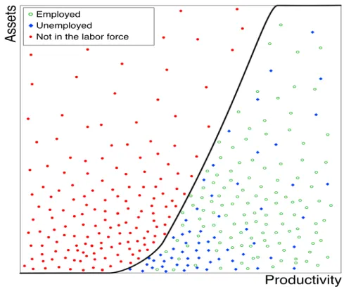
The individual will stochastically transit among the three labor market states—employment, unemployment and non-participation. Idiosyncratic productivity and assets determine whether an individual would like to work given the opportunity, and frictions influence whether an individual who prefers to work will be employed or unemployed. Figure 1 shows a stylized version of the optimal decision rule for participation and distribution of individuals across three labor market states that would come out of a model of the sort considered here.

The participation decision is captured by an upward-sloping curve in (a, z) space with the individual wanting to work, i.e., participating, for (a, z) combinations that are below the line. Specifically, Figure 1 says that higher productivity and lower assets both make it more likely that an individual will participate, holding all else constant. The former effect represents a standard intertemporal substitution effect: holding all else constant the individual prefers to participate when the return to market work (relative to the opportunity cost of working) is high. The latter effect represents an income effect: holding all else constant, the greater the wealth that an individual has, the less likely it is that he or she will work. For future

6

Given evidence from time use data on the amount of time devoted to search, we think it is reasonable to assume that the cost of active search is very small. In our earlier work we argued that a more natural way to connect the model to the data was to adopt a more inclusive definition of unemployment in the data, based on the desire to work rather than active search. Nonetheless, we found that the broader definition was not substantively important either in terms of the features in the data or the ability of the model to account for the data. We revert to the standard definition of unemployment in this paper because of the difficulty in getting a longer time series for flows between the states with the broader measure.

Figure 1: Stylized optimal decision rule for participation and the distribution of individuals across three labor market states.

reference it is important to note that the position of the participation boundary in Figure 1 is determined by the settings for market conditions.

3.3 Using the Model to Address Aggregate Gross Worker Flows

To this point we have talked about the situation of an individual worker and described how this individual will transition between the three labor market states. A natural way to use this model to examine the implications for aggregate gross worker flows is to assume that there are a large number of workers, each of whom is just like the individual we described above, and that all of the shocks are idiosyncratic. Given a set of market conditions, we could then look for a stationary distribution of the individuals. In this stationary distribution there would be an invariant distribution of individuals over the individual states: assets, idiosyncratic productivity and whether employed last period.

bound-ary in Figure 1 would be the same for all individuals. Given a participation boundbound-ary and the invariant distribution over pairs (a, z), we can determine the participation rate by integrating the distribution above the boundary. Gross flows between participation and non-participation occur when individuals transit across the boundary. Loosely speaking, holding the stochastic process for idiosyncratic shocks fixed, these flows will depend on how much mass is near the boundary. Additionally, for those individuals who are above the boundary and hence are par-ticipating, how they are distributed between employment and unemployment will influence the magnitude of the flows between these two states and non-participation.

One of the key exercises that we carry out in this paper is to examine how fluctuations in market conditions influence gross worker flows, specifically those that involve flows between participation and non-participation. Figure 1 offers a useful framework for organizing one’s thinking about this issue. In particular, the figure suggests that in response to a one time change in market conditions there will be two distinct effects on flows between participation and non-participation. First, and as noted previously, a one-time change in market conditions will lead to a one-time movement in the participation boundary. This will necessarily lead some individuals to change their participation status, even holding their individual state constant. But note that this effect is only present in the period of the change in market conditions. The second effect has to do with the changes in the mass of individuals who are near the boundary, and in particular, how those individuals who are located just above the boundary are distributed between E and U. Unlike the first effect, which was a one-time change in flows, this effect will be persistent. Additionally, this effect will have a dynamic component, since the distribution of individuals near the boundary between E and U will also have some dynamics. For example, suppose that the participation region expands. At the time of the change, all of those individuals who are just above the new participation boundary will necessarily be looking for jobs, since prior to the change they did not desire employment, and a fraction of them will not find a job immediately. But as time passes, the

dynamics of job finding, job loss and idiosyncratic shocks will lead to a stationary distribution for these individuals in which a smaller fraction of them are unemployed.

4

Fluctuations in Gross Worker Flows

Our main goal is to examine whether our labor supply model of gross worker flows can match the properties of fluctuations in gross worker flows exhibited in Table 1 when subjected to empirically reasonable aggregate shocks to “market conditions”, by which we mean prices and frictions. We emphasize that our goal here is not to find a full general-equilibrium model of what explains the variation in market conditions—what makes wages higher some times than other times and jobs easier to find some times than other times. This would necessitate taking a stand on the relative importance of different mechanisms in the aggregate economy and those mechanisms are not our priority here. Rather, we seek parsimonious representations of market conditions that influence households systematically in their labor supply decisions. In this section we describe the method that we use to achieve this goal.

4.1 Modeling Shocks to Market Conditions

There are a few different ways that one might proceed. One strategy would be to estimate the model using some type of simulated moments estimator on time series data. Rather than pursue that route we adopt a much simpler and more transparent approach that we think offers some important insights into the role that different driving forces play in shaping the cyclical properties of gross worker flows. Specifically, given that our focus is on business cycle fluctuations and that a key feature of business cycles is comovement among series, we effectively focus on perfectly correlated movements in market conditions that reflect business cycle movements and ask whether such movements can account for business cycle fluctuations in gross worker flows if the relative variances of the movements in each variable are set to empirically reasonable values.

a Markov process, with the prices and frictions all being functions of this aggregate state s. Relative to this specification we introduce one additional element, described below, that serves two purposes. First, it will provide a particular discipline to the movements in w and r. Second, it will provide for some feedback effects from frictions to prices, in the sense that if changes in frictions lead to increases in employment holding all else constant, we will impose that this leads to a reduction in wages due to a decline in the marginal product of labor. Although it will turn out that these feedback effects are minimal, we thought it was important to allow for them in some fashion.

We impose these connections between the various components of market conditions by positing an aggregate production function and requiring that changes inwandrare mutually consistent with changes in factor inputs under the assumption that factor prices are equal to marginal products. To generate shocks to w we assume that this aggregate production function is subject to total factor productivity (TFP) shocks, denoted byZ. So, rather than considering shocks to two prices and two frictional parameters, our method involves shocks to three values: a fictional aggregate TFP and the two frictions. We emphasize that we do not interpret the TFP shock in a literal sense; rather it is simply a vehicle to generate fluctuations in prices and impose some discipline on feedback effects from frictions to prices.7 _{By virtue}

of having a hypothetical aggregate production function in the background, we can generate time series for output and so report correlations of labor market variables with output. We describe the implementation of this procedure in more detail in the Appendix A.4.

4.2 Calibrating the Stationary Distribution

In this section we calibrate the parameters of our model so that in the stationary distribution with constant market conditions the flows of workers across labor market states does a good job of matching the average levels of gross worker flows in the data. The procedure draws

7

An interesting and perhaps simpler alternative would be to simply posit a fixed real returnrand assume a downward sloping labor demand function subject to a shock.

heavily on the procedure outlined in Krusell et al. (2011), so we just sketch it here.

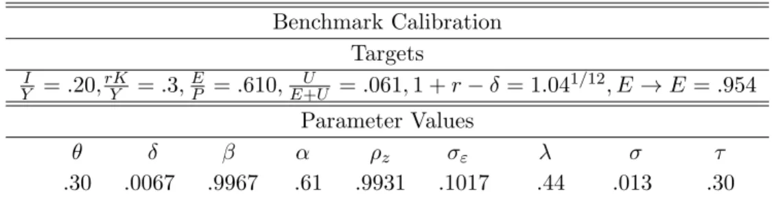
The model has ten parameters that need to be assigned: preference parameters β and α, idiosyncratic shock parameters ρz and σε, frictional parameters σ and λ, the tax rate τ,

the transfer T, and prices r and w. Because data on labor market transitions are available monthly, we set the length of a period to be one month. The wage rate per efficiency unit,w, can be normalized to one. As is standard in the macro literature, we setr so that the annual rate of return on assets is 4%. Given this rate of return and the model’s other parameters, the value of the discount factor β will influence the level of average asset holdings in the stationary distribution. In a general equilibrium setting this would in turn have implications for the value of r. Although our analysis is partial equilibrium in nature, we choose β so that the amount of capital accumulated in steady state would be consistent with an annual return of 4% assuming a standard production function.8 _{We setτ =.30 and then setT to be}

consistent with a balanced budget in the stationary distribution.9 _{The preference parameter}

α, which captures the disutility of working, is set so that the employment to population ratio in the stationary distribution is equal to .61. This is the value of the employment to population ratio for the population aged 16 and older for the period 1968–2009.10

It remains to choose values forλ,σ,ρzandσε. Recall that our idiosyncratic shock process

should be viewed as a composite of all idiosyncratic shocks that affect the static return to working versus not working. Shocks to wages are of course only one such component. However, since these are the shocks that we have the best measures of, our benchmark specification calibrates the shock process based on estimates of idiosyncratic wage shocks. Specifically, we choose values forρz andσεbased on Floden and Linde (2001), who estimated

8

Specifically, we calculate this by assuming a Cobb-Douglas production function with capital share equal to.3 and a monthly depreciation rate of.0067.

9

Following the work of Mendoza, Razin, and Tesar (1994) there are several papers which produce estimates of the average effective tax rate on labor income across countries. Minor variations in methods across these studies produce small differences in the estimates, but.30 is representative of these estimates.

10

We calibrate to values for the period 1968–2009 because this is the period for which we have consistent measures of labor market flows.

ρz =.92 and σε=.21 expressed on an annual basis.11

There is an intimate connection between λand the unemployment rate in the model. If λ= 1 then unemployment will be zero, since everyone always has the opportunity to work. We therefore chooseλso that the steady state unemployment rate matches the average value for the unemployment rate in the U.S. data for the period 1968–2009, which is .061. We choose σ to target the average flow rate out of employment over our sample period, which is 3.6%. We target this rate based on our belief that the employment state is the one subject to the least amount of measurement error.

Table 2 summarizes the calibrated values and the various targets used in the calibration. Table 2

Calibration Targets

E

P =.610, U

E+U =.061,1 +r = 1.04

1/12_{, E →E=.964}

Parameter Values

β α ρz σε λ σ τ

.9967 .61 .9931 .1017 .44 .013 .30

The labor market flows in our calibrated model and the data are displayed in Table 3. Table 3

Gross Worker Flows in the Data and the Model

US 1968-2009 Model

FROM TO FROM TO

E U N E U N

E 0.954 0.016 0.030 E 0.954 0.007 0.039 U 0.270 0.508 0.222 U 0.396 0.505 0.099 N 0.048 0.027 0.925 N 0.035 0.044 0.921

Overall the model does a reasonable job of capturing the salient features of the data. Specifically, it does a good job of capturing the degree of persistence in each of the three states. The one major discrepancy is that the model does not generate enough flows from U toN. Given our strategy of targeting the stock of workers inU, this necessarily implies that

11

Krusell et al. (2011) showed that the ability of the model to account for the flows between states remains relatively unchanged over a wide range of values ofρandσε. What mattered most was thatρwas reasonably

persistent (at least.5), but not too close to being a unit root (say less than .97), and that σε was not too

the other flow out ofU (i.e., the flow fromU toE) must also be off. It has long been known that that classification errors lead to spurious flows, especially between unemployment and not in the labor force (see, e.g., Poterba and Summers (1986)). The survey that Poterba and Summers used to estimate the extent of classification error on transition rates was discontin-ued shortly thereafter, so one cannot use their procedure to produce an adjusted time series. More recently, Elsby, Hobijn, and S¸ahin (2012) devise another procedure for purging the data of spurious flows that one can carry out over a longer time period. They estimate that the “true” transition rate from U toN is equal to .14. In Appendix A.2 we show that with an empirically plausible amount of measurement error the model does a much better job of matching the flows betweenU andN. While classification error is important in matching the average behavior of flows in the data, we also show in Appendix A.2 that it is not important for our key findings about business cycle fluctuations. And as noted previously, the work by Elsby, Hobijn, and S¸ahin (2012) shows that classification error does not have an important impact on cyclical properties.

4.3 Calibrating Shocks to Market Conditions

Having described the procedure that we will follow to examine the model’s implications for business cycle fluctuations in gross worker flows, it remains to describe how we determine the parameters of the stochastic process for market conditions. As is standard in the business cycle literature with heterogeneous agents, we assume that the shocks to market conditions follow a two state Markov process. We will refer to one state as the “good” state and the other state as the “bad” state. The good state will have a high value ofZ (and hence also for wandr), a high value for the employment arrival rateλ, and a low value for the employment separation rate σ. We denote the two possible realizations for the market conditions shock as (ZG_{, λ}G_{, σ}G_{) and (Z}B_{, λ}B_{, σ}B_{). We parameterize the TFP shock as Z}G _{= 1 +ε}Z_{, and}

ZB _{= 1−ε}Z_{, and the other two shocks as λ}G _{= λ}∗ _+ελ_{, λ}B _{= λ}∗ _−ελ_{, σ}G _{= σ}∗ _−εσ_,

transition rates. We assume that the transition matrix for the Markov process is symmetric, with diagonal element denoted by ρ.

In our model, both the level and fluctuations in fU E closely mimic the level and

fluctu-ations in λ. For this reason we choose the value ofελ _{so that the fluctuations inf}

U E in the

simulated model match the standard deviation of the fluctuations infU E found in US data.

This leads toελ _{=.069. Controlling for λ, which influences the impact of time aggregation}

on measured fEU, the level and fluctuations infEU closely follow the level and fluctuations

inσ, so we chooseεσ _{=.00051 so as to match the fluctuations in f} EU.

We choose the value ofεZ_{so as to target the volatility of wages. While market conditions}

are defined by the value ofw, the wage per efficiency unit of labor services, this is not directly observable in the data. Instead, what we observe in the data is the average value of the wage payment per unit of time, which we will refer to as ¯w. In our model this is given by the ratio of total wage payments to the level of employment. This is the concept of wages that we target in our calibration. Gertler and Trigari (2009) report that the relative standard deviation of real hourly wages for production workers relative to nonfarm business output is .52. Our benchmark model yields a ratio of .49 for this statistic. It turns out that when we match this value our model will generate employment fluctuations that are the same as those found in the data. This requires εZ _=.0287.

In our model we can clearly distinguish between fluctuations in the wage per efficiency unit of labor services, which we denoted by w, and fluctuations in the value of the average wage observed in the economy, which we will denote by ¯w. A sizable literature (see, e.g., Bils (1985), Keane, Moffitt, and Runkle (1988) and Solon, Barsky, and Parker (1994)) has argued that cyclical fluctuations in ¯w are significantly less than fluctuations in w due to cyclical changes in the composition of the employment pool. Because our model has heterogeneous workers we can assess the extent of this bias in our benchmark model. We report the details later, but note here that in our benchmark model the size of the negative composition bias

is substantial.

5

Results in the Benchmark Model

In this section we report the results of our study. We begin by examining the ability of the model to account for cyclical movements in stocks, and then move on to examine cyclical movements in gross worker flows.

5.1 Cyclical Properties of Stocks

We begin by assessing the ability of the model to match the cyclical movements in the three labor market stock variables—employment, unemployment rate and the participation rate. Table 4 shows the results for the benchmark model and the data.

Table 4

Behavior of Stocks in Benchmark Model

Volatilities Correlations Autocorrelations std(x) corrcoef(x, Y) corr(x, x−1)

u lf pr E u lf pr E u lf pr E Data .12 .003 .011 −.87 .46 .84 .92 .72 .95 Model .13 .004 .011 ₋.98 .56 .97 .80 .68 .78

As noted earlier, the value of wage fluctuations that we targeted in our benchmark spec-ification turns out to generate exactly the same fluctuations in employment as found in the data. However, it is noteworthy that the model also does a good job of accounting for the size of fluctuations in both unemployment and participation. Moreover, it also correctly accounts for the fact that employment is strongly procyclical, the unemployment rate is strongly countercyclical, and the labor force participation rate is weakly procyclical. While the model slightly understates persistence in unemployment and employment, its prediction for the persistence of quite accurate.

To understand the economic forces underlying these movements in labor market stocks, it is instructive to separately consider the role of price versus job availability shocks. Table

5 presents results for the wage shocks and friction shocks taken separately.12

Table 5

Behavior of Stocks to Price and Job Availability Shocks

Volatilities Correlations Autocorrelations std(x) corrcoef(x, Y) corr(x, x−1)

u lf pr E u lf pr E u lf pr E

data .12 .003 .011 −.87 .46 .84 .92 .72 .95

wage shocks .03 .010 .011 ₋.55 .94 .96 .37 .71 .75

job availability shocks .11 .007 .002 ₋.90 ₋.80 .45 .79 .72 .52 The striking finding in Table 5 is that neither price nor job availability shocks individually are capable of reproducing the key cyclical features found in the data. Specifically, with job availability shocks only we see that participation not only fluctuates too much but is strongly countercyclical instead of weakly procyclical. Although this specification does a good job of matching fluctuations in the unemployment rate, employment fluctuations are very small relative to their value in the data. In contrast, with wage shocks only, participation becomes procyclical, but still fluctuates too much relative to the other series. And although employment fluctuates the same as in the data, unemployment hardly fluctuates at all.

We conclude that in the context of our model of gross labor market flows, both price and job availability shocks are essential in accounting for the patterns found in the data. Although our analysis is only partial equilibrium in nature, this finding has important implications for the mechanisms that can drive labor market fluctuations over the business cycle in a general equilibrium setting. For example, the fact that the model with friction shocks only cannot match the behavior of labor market stocks suggests that models in the spirit of Mortensen and Pissarides featuring TFP or some other supply shocks but with perfectly rigid wages are not sufficient to capture the behavior of the three labor market stocks. Previous researchers such as Hall (2005) and Shimer (2005) had argued that this class of models offered a good account of labor market dynamics in the context of a model in which participation is fixed

12_{As noted earlier, even in the job availability shocks only case, our method will allow for changes in prices} induced by changes in factor inputs. It turns out that these effects are very small, so that this case effectively corresponds to a case in which prices are constant.

exogenously. Although participation does not fluctuate too much over the cycle in the data, our analysis shows that exogenously shutting down this margin is far from innocuous for understanding employment fluctuations. Why does the presence of the participation margin have such large effects on employment fluctuations in the face of shocks to frictions? This is the question we turn to next.

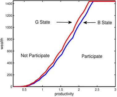
As a first step in exploring the underlying economic mechanism, consider how the par-ticipation region adjusts as job availability parameters change from their level in the bad aggregate state to their level in the good aggregate state. We analyze this separately for the job availability shocks and wage shocks. Figure 2 illustrates this by plotting the participa-tion boundary for the two different realizaparticipa-tions of the aggregate job availability shocks when prices are constant (that is, corresponding to the third row of Table 5), evaluated at the mean level of the other individual states.

Figure 2: Cut-off wealth and productivity levels for the model with job availability shocks only

0.5 1 1.5 2 2.5 3

0 200 400 600 800 1000 1200 1400

productivity

wealth

Not Participate Participate G State B State

The important message from Figure 2 is that when job availability worsens, thereby making it more difficult to obtain employment, individuals respond by expanding the set of

individual states in which they will work.13 _{This manifests itself in two ways: individuals who}

are employed will be less likely to move out of employment in response to idiosyncratic shocks, and some individuals who are not employed will decide to accept employment opportunities under conditions that they previously would not.

This effect is intuitive. A key desire for individuals in this economy is to arrange the timing of work to coincide with periods of high individual productivity. Frictions interfere with an individual’s ability to achieve the desired timing. When frictions become more severe, individuals respond by expanding the set of conditions under which they will work if given the opportunity, i.e., by becoming less choosy about when they work. The implication is that participation will be countercyclical in the presence of shocks to frictions. While the magnitude of this effect will depend on the density of individuals around the boundary of the two regions, this figure illustrates the main economic mechanism at work. It is important to emphasize that the magnitude of this effect depends critically on the size of income and substitution effects in labor supply. In particular, a model with linear utility and hence no income effects will underestimate the desire of individuals to work more in response to changes that lower income.

The second class of business cycle models that the results in Table 5 cast doubt on are those implicit in standard real business cycle models. Standard real business cycle models such as Hansen (1985) contain no frictions and do not allow one to separate the non-employed into the unemployed and non-participants. Our model does permit this, but the price shocks only row in Table 5 shows that if job availability is constant over the business cycle, then the model does not deliver sufficient movement in unemployment. One recurring critique of real business cycle models has been that they do not account for unemployment, and our analysis supports this critique. To understand the underlying economics, it is again instructive to examine how decision rules and flows are affected by the wage shocks when job availability is

13_{In Krusell et al. (2010) we demonstrated that this effect was quantitatively important in terms of steady} state outcomes. Here we see that the effect is quantitatively significant in a business cycle context as well.

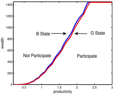
constant (that is, corresponding to the second row in Table 5). Figure 3 plots the behavior of the decision rule for participation that is equivalent to Figure 2.

Figure 3: Cut-off wealth and productivity levels for the model with price shocks only

0.5 1 1.5 2 2.5 3

0 200 400 600 800 1000 1200 1400

productivity

wealth

G State B State

Participate Not Participate

This figure illustrates the standard intertemporal substitution effects present in standard real business cycle models: when wages are high individuals choose to work more, which corresponds to expanding the set of individual states in which they desire to work. This is the effect that leads to procyclical employment and participation. To the extent that the employment responses reflect standard intertemporal substitution, it may seem a curiosity that unemployment in this exercise does fluctuate countercyclically. We return to this issue later when we discuss our results in relation to those in Veracierto (2008).

To summarize, we have shown that our model of gross worker flows can account for fluctuations in the three labor market stocks given empirically reasonable fluctuations in prices and job availability. Of particular importance is the finding that neither job availability or price shocks alone can generate the business cycle patterns found in the data.

5.2 Cyclical Properties of Gross Flows

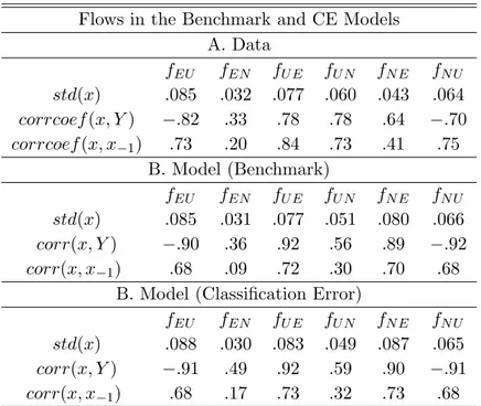
Having established that our labor supply model of gross worker flows can account for cyclical properties of labor market stocks given empirically reasonable shocks to market conditions, we now raise the bar in evaluating the model’s ability to account for the key features of the data and ask whether it can also account for the cyclical behavior of gross worker flows. Table 6 shows the results for the cyclical properties of transition probabilities in our benchmark model. For ease of comparison, we also repeat the properties of the data that were previously reported in Table 1.

Table 6

Gross Worker Flows in the Benchmark Model A. Data

fEU fEN fU E fU N fN E fN U

std(x) .085 .032 .077 .060 .043 .064 corrcoef(x, Y) −.82 .33 .78 .78 .64 −.70 corrcoef(x, x−1) .73 .20 .84 .73 .41 .75

B. Model

fEU fEN fU E fU N fN E fN U

std(x) .085 .031 .077 .051 .080 .066 corr(x, Y) −.90 .35 .92 .56 .89 −.92 corr(x, x−1) .68 .09 .72 .30 .70 .68

This table shows that the model does a good job of accounting for the key patterns. It captures the countercyclicality of unemployment inflows (EU and N U flow rates), procycli-cality of unemployment outflows (U Eand N U flow rates) and mild procyclicality of the EN flow rate. The model delivers a volatility and correlation (with output) for fN E that are

somewhat too high. We discuss this shortcoming in more detail below.

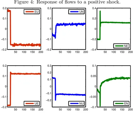
To examine the economics behind the cyclicality of the gross flows it is instructive to focus on the transition dynamics in the various flows when the economy has been in the bad state for many periods and then receives a good shock that persists for many periods. Figure 4 shows the responses of the transition rates as the economy moves from bad times to good times.

Figure 4: Response of flows to a positive shock.

50 100 150 200

−0.2 −0.1 0 0.1 0.2 EU

50 100 150 200

−0.2 −0.1 0 0.1 0.2 UN

50 100 150 200

−0.4 −0.2 0 0.2 0.4 NE

50 100 150 200

−0.2 −0.1 0 0.1 0.2 UE

50 100 150 200

−0.2 −0.1 0 0.1 0.2 0.3 NU

50 100 150 200

−0.1 −0.05 0 0.05 0.1 EN

5.2.1 Understanding the Flows between E and U

We begin with the flows between E and U, which are the simplest. To move from U toE across adjacent periods requires that two things happen: the individual must receive a work opportunity (which happens with probability λ) and not suffer an idiosyncratic shock that changes their desire to work. The change in the probability of the second event as we move from bad to good market conditions is of second order importance. So the dominant effect is the increase in λ, implying an increase in the transition rate from U toE.

To move from E toU across adjacent periods, three things must happen: a worker must suffer a separation, not receive a new employment opportunity, and not suffer an idiosyncratic shock that changes their desire to work. Again, the change in the probability of the third event is of second order importance. The probability of the first two events isσ(1₋λ), which is clearly lower in the good state, implying a decrease in the E toU flow rate.

In this context, and as a side issue, it is interesting to assess the relative importance of the changes in σ and λon the observed change in the flows between E and U. To do this we simulate the model with shocks to only one friction at a time and compute summary

statistics for the gross flows. The results are in Table 7. Table 7

Contribution of the Shocks: Flows std(x) corrcoef(x, Y) fEU fU E fEU fU E

Data .085 .077 −.82 .78 All .085 .077 ₋.90 .92 λ .069 .076 −.66 .73 σ .033 .011 ₋.48 ₋.02

The interesting result here is that even when there are only shocks to λ, so that σ is constant, the model accounts for roughly 80% of the volatility infEU. This reflects the time

aggregation that is implicit in our model: when λis low it is more likely that a worker who experiences an employment separation will remain in the unemployment state. Note that in the specification with only shocks to σ there is also an effect on the transition rate from U toE. This may at first seem somewhat surprising. However, this effect is due to a one-time effect associated with changes in the value of σ. The nature of the effect is that during good times (i.e., whenσdecreases), some people move from participation to non-participation due to the fact that as it becomes easier to work when one desires, one becomes more particular about timing periods of work with high values of the idiosyncratic shocks. As a result, during the period in whichσ changes from high to low, some of the previously unemployed move to non-participation and hence even though they receive employment opportunities they choose not to work. This causes a one-time reduction infU E. The fact that it is a one-time reduction

is evident in the very low correlation betweenfU E and output in the case of shocks only to

σ.

5.2.2 Understanding the Flows between E and N

Returning to the transition dynamics in Figure 4, we next consider the change in the tran-sition rate from N to E. Note that there is a persistent increase in this flow, but that the increase in the initial period of the shock is even larger than the persistent effect. The per-sistent increase is due to the change in frictions. To move from N to E two things must

happen: the individual must experience a change in their idiosyncratic shock that makes them want to work, and they must also receive an employment opportunity.14 _{Once again,}

the change in the probability of receiving an offer is the dominant effect, so that when λ increases, so does the probability of transiting from N to E. To understand why the initial effect is significantly larger, note that when market conditions change to the good state, the participation region for individual workers expands. Hence, in the initial period the pool of potential workers who transition fromN toE includes not only those who transit across the boundary between the participation and non-participation region, but also those who enter the participation region because of the change in the position of the boundary. Because the effect of the change in the boundary only occurs in the initial period of the change, this causes an initial spike in theN toE flow.

Next we consider the movement from E toN. Note that the persistent effect is positive whereas the immediate effect is negative. To understand why the immediate and persistent effects are of different sign it is important to isolate the two separate effects that we noted earlier: the effect due to the one-time change in the participation boundary versus the persis-tent and dynamic effect associated with the changing mass of employed individuals who are close to the participation boundary. In the stationary distribution, with a fixed decision rule that defines the boundary between the participation region and the non-participation region, the flow from E toN occurs when an employed individual crosses the boundary. The flow is therefore determined by the mass of employed individuals that are close to the boundary. When the economy is hit with a positive shock to market conditions, the participation region expands, thereby making it less likely that an employed individual who is initially near the older boundary will actually exit the participation region.

The second effect has to do with changes in the mass of employed individuals who are

14

As explained in the theoretical section above, there are also predictable movements over time across the boundary due to asset accumulation (inE) or decumulation (in N), as well as a drift inz toward its mean. These are both small quantitatively and so we do not focus on them in this discussion.

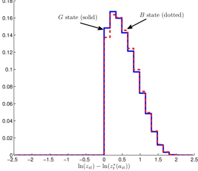
near the boundary. As noted earlier, this effect will have a dynamic component since the distribution of employed individuals “fills in” the area between the two boundaries over time. The long run effect is purely determined by the movement of employed individuals across the boundary in the new stationary distribution. In good times, it turns out that there are relatively more marginal workers in the employment pool, and these workers are more likely to experience a transition to out of the labor force. In order to illustrate this point, we draw Figures 5 to 7 that describe the distribution of workers, in terms of the distance from the participation boundary, in good state and in bad state.

Figure 5: The distribution of “distance to indifference”: E workers

−2.5 −2 −1.5 −1 −0.5 0 0.5 1 1.5 2 2.5

0 0.02 0.04 0.06 0.08 0.1 0.12 0.14 0.16 0.18

ln(zit)−ln(z∗t(ait))

Gstate (solid) Bstate (dotted)

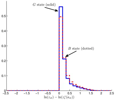
In the model, a worker’s situation described as a point in (a, z) space. In order to describe the distribution of workers’ distance from the participation boundary in a one-dimensional metric, we measure the distance in terms of “z-equivalence”. In particular, we ask each worker (worker i at time t) a question: “how much does your ln(zit) have to be higher to

Figure 6: The distribution of “distance to indifference”: U workers

−2.5 −2 −1.5 −1 −0.5 0 0.5 1 1.5 2 2.5

0 0.1 0.2 0.3 0.4 0.5

ln(zit)−ln(z∗t(ait))

Gstate (solid)

Bstate (dotted)

Figure 7: The distribution of “distance to indifference”: N workers

−2.5 −2 −1.5 −1 −0.5 0 0.5 1 1.5 2 2.5

0 0.05 0.1 0.15 0.2 0.25

ln(zit)−ln(z∗t(ait))

Gstate (solid)

ln(zit)−ln(z∗t(ait)), wherezt∗(a) is the level ofzthat makes a worker with wealthaindifferent

at timet(i.e. the function representing the participation boundary att). Then we count the number of workers whose ln(zit)−ln(z∗t(ait)) fall into each bin (the total number of people

in each state is normalized to one).

Each figure has two histograms: one for the good aggregate state and one for the bad aggregate state.15 _{Looking at the E pool (Figure 5), we see that there are more marginal}

workers—workers with a short distance to the boundary—in good times than in bad times. The reason why there are more marginal workers in good times is the change in job availabil-ity. If the employment opportunity arrival rate is relatively high, then new hires will be a greater fraction of all employment. New hires in our model are disproportionately composed of individuals who are close to the boundary, that is, individuals who previously did not want to work but received an idiosyncratic shock that pushed them over the boundary. Because individuals who are close to the boundary are more likely to receive a new realization that causes them to cross the boundary, the result is that we now have greater flows from E to N.

5.2.3 Understanding the Flows between N and U

Finally, consider the flows between N and U. First, the change in the flow from N to U is basically the mirror image of the change in the N to E flow, since this reflects the case in which an individual changes their desire to work but does not receive a work opportunity.

As for the flow from U to N, the reasoning is similar to that for the E to N flows. In particular, the immediate effect is a decrease due to the expansion in the size of the partic-ipation region. The persistent effect is again positive for reasons involving the composition of the unemployment pool. Referring back to Figure 6, we see that there are more marginal workers in good times. Specifically, since in the good state unemployed workers leave for

15_{In order to look at the “long-run” effect, both periods are chosen so that each is after 80 consecutive} periods of the same aggregate state.

employment more quickly, the pool of unemployed individuals is relatively more dominated by individuals who have just entered unemployment. Since employed workers are less likely to enter unemployment in good times, new entrants to unemployment are dominated by in-dividuals that transition from N to U. But these individuals are more likely to be close to the boundary, making them more susceptible to a transition that puts them back in the N state. The reason that the persistent effect is relatively larger in this case than in the case of the E toN flow has to do with the fact that the persistence in the unemployment state is much lower than the persistence in the employment state, so that the composition effects are relatively more important. This model feature is consistent with Elsby, Hobijn, and S¸ahin (2012), who show that the composition of the unemployed pool shifts towards more “attached” workers during recessions, where the most important dimension of attachment is prior employment status. They show that this mechanism accounts for around 1/3 to 2/3 of the decline in U toN flow rate during recessions.

We noted earlier that the volatility of fN E in the model is significantly larger than it

is in the data, and that its correlation with output is is also somewhat high relative to the data. Looking at Figure 4, it is apparent that one of the sources of the large volatility is the large initial jump in fN E that occurs immediately upon impact of the new realization of

market conditions. While we do not pursue it here, it is perhaps reasonable to think that this movement of individuals from out of the labor force into employment may be spread over a slightly longer period, and if this were the case, then the standard deviation would presumably drop considerably. This would also diminish somewhat the correlation between fN E and output.

The above discussion has focused on describing the intuition for the qualitative patterns found in Figure 4. These qualitative patterns can in turn be connected with the correlations that we see in Table 6. We conclude that the economics implicit in the model that is responsible for these patterns is quite straightforward, and for this reason we think the results

are a robust feature of our simple model of worker flows. Of course, the extent to which the model can reproduce the quantitative features of fluctuations in gross flows depends not only on the qualitative patterns but also the quantitative magnitudes of the various effects. It is reasonable to think that a key factor for the quantitative results is the mass of individuals that are near the participation boundary. In this regard, the discipline in our quantitative work derives from the fact that our steady state model is consistent with the average level of gross flows. In this sense, our model captures the amount of workers that are close to the boundary.

5.3 Fluctuations in Wages and Composition

When we discussed calibrating shocks to wages we noted that there were several different notions of wages that were of interest and that had received attention in the literature. Here we report the properties of different wage measures. Results are reported in Table 8.

Table 8 Behavior of Wages

Volatility: std(x)/std(Y) Correlation: corrcoef(x, Y)

w w¯ wnew w w¯ wnew

Benchmark .63 .49 .77 .99 .97 ₋.14

As noted earlier, in our benchmark model, the standard deviation of the average wage relative to output is .49. Table 8 shows that this is roughly 20% lower than the volatility of the wage per efficiency unit of labor services, which has a standard deviation relative to output of.63. Both of these measures are highly correlated with output. The reason for this difference is that during good times, the participation region expands to include individuals with lower values of idiosyncratic productivity. Interestingly, fluctuations of the average wage for all new hires is significantly more volatile—by roughly 50% so—than the average wage. Note that this is due entirely to composition effects and is not because wage setting differs for new hires relative to existing workers. Haefke, Sonntag, and van Rens (2008) documented that wages of new hires are more volatile than wages for existing workers and

argued that this had important implications for wage setting and the equilibrium fluctuations in standard matching models. Gertler and Trigari (2009) cautioned that this conclusion might be premature if composition effects were significant. In our benchmark model these composition effects are large. Note, however, that the wage series for new hires in our model is not very highly correlated with output.

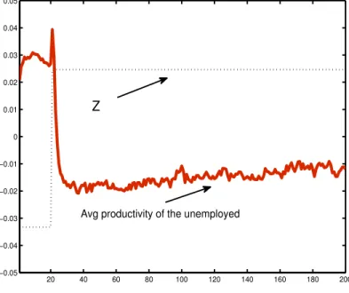
The above discussion of wage fluctuations is ultimately about composition changes in the employment pool. There is also a literature on the cyclical composition of the unemployment pool. Consistently with earlier arguments in Solon, Barsky, and Parker (1994), recent work by Mueller (2010) argues that the average quality of an unemployed worker rises significantly (by 2-3%) in recessions. His measure of the productivity of an unemployed worker is based on the worker’s most recent wage as employed (typically 8 months earlier). Our model reproduces these findings. Figure 8 shows the change in the average worker productivity for all unemployed workers as the economy experiences the same transition as pictured in Figure 4.

Figure 8: Response of average productivity of unemployed workers to a positive shock.

20 40 60 80 100 120 140 160 180 200 −0.05

−0.04 −0.03 −0.02 −0.01 0 0.01 0.02 0.03 0.04 0.05

Avg productivity of the unemployed