Testing deviations from Lambda CDM with growth rate measurements from six large-scale structure surveys at z=0.06-1

(1)

Testing deviations from

CDM with growth rate measurements from six

large-scale structure surveys at

z

=

0 .

06–1

Shadab Alam,

1,2‹

Shirley Ho

1,2

and Alessandra Silvestri

3 1_{Department of Physics, Carnegie Mellon University, 5000 Forbes Ave., Pittsburgh, PA 15217, USA}

2_{McWilliams Center for Cosmology, Carnegie Mellon University, 5000 Forbes Ave., Pittsburgh, PA 15217, USA} 3_{Institute Lorentz, Leiden University, PO Box 9506, NL-2300 RA Leiden, the Netherlands}

Accepted 2015 December 12. Received 2015 December 5; in original form 2015 September 27

A B S T R A C T

We use measurements from thePlancksatellite mission and galaxy redshift surveys over the last decade to test three of the basic assumptions of the standard model of cosmology,CDM (cold dark matter): the spatial curvature of the universe, the nature of dark energy and the laws of gravity on large scales. We obtain improved constraints on several scenarios that violate one or more of these assumptions. We measurew0= −0.94±0.17 (18 per cent measurement) and 1 +wa =1.16±0.36 (31 per cent measurement) for models with a time-dependent

equation of state, which is an improvement over current best constraints. In the context of modified gravity, we consider popular scalar–tensor models as well as a parametrization of the growth factor. In the case of one-parameterf(R) gravity models with aCDM background, we constrainB0<1.36×10−5_(1σ_{C.L.), which is an improvement by a factor of 4 on the current} best. We provide the very first constraint on the coupling parameters of general scalar–tensor theory and stringent constraint on the only free coupling parameter of Chameleon models. We also derive constraints on extended Chameleon models, improving the constraint on the coupling by a factor of 6 on the current best. The constraints on coupling parameter for Chameleon model rule out the value ofβ1 =4/3 required forf(R) gravity. We also measure γ = 0.612 ± 0.072 (11.7 per cent measurement) for growth index parametrization. We improve all the current constraints by combining results from various galaxy redshift surveys in a coherent way, which includes a careful treatment of scale dependence introduced by modified gravity.

Key words: gravitation – galaxies: statistics – cosmological parameters.

1 I N T R O D U C T I O N

Since its development a century ago, General Relativity (GR) has consistently provided a very successful framework to describe the evolution of our Universe (Peebles1980; Davis & Peebles1983). Nowadays, the prediction of GR for the growth of the large-scale structure that we observe around us is reaching great precision as cosmic microwave background (CMB) measurements are provid-ing us with impressively accurate estimates of the cosmological pa-rameters (Planck Collaboration2015a). Yet, the excitement about the advances of observational cosmology is accompanied by the awareness that we face some major challenges. While the standard cosmological model, based on the laws of GR, provides a very good fit to existing data, it relies on a universe of which we

_E-mail:_{[email protected]}

stand only∼5 per cent of the content. The remaining energy budget comes in the form of dark matter (∼27 per cent), responsible for the clustering of structure, and the cosmological constant(Einstein

1915,∼68 per cent), responsible for the phase of accelerated ex-pansion recently entered by the universe. In particular, the physical understanding of cosmic acceleration represents one of the most important challenges in front of modern physics. While is in good agreement with available data, e.g. baryon acoustic oscilla-tions (BAO; Cole et al.2005; Eisenstein et al.2005; H¨utsi2006; Kazin et al.2010; Percival et al.2010; Reid et al.2010; Anderson et al.2014a,b; Aubourg et al.2015), supernovae (SNe; Perlmutter & Schmidt2003; Conley et al.2011; Goobar & Leibundgut2011; Suzuki et al.2012; Rodney et al.2014) and CMB (Planck Collabo-ration2015a;WMAP9, Bennett et al.2013) observations, it suffers from the coincidence and fine tuning problems (Weinberg1989; Carroll2001). Several alternatives tohave been proposed in the two decades since the discovery of cosmic acceleration (Riess et al.

2016 The Authors

at Leiden University on December 14, 2016

http://mnras.oxfordjournals.org/

(2)

1998; Perlmutter et al.1999), and they can be roughly divided into two classes. The first class, to which we will refer asmodified grav-ity (MG), corresponds to modifications of the laws of gravity on large scales, designed to achieve self-accelerating solutions when matter becomes negligible (Silvestri & Trodden2009; Clifton et al.

2012); alternatively, one can introduce a dynamical degree of free-dom, commonly dubbeddark energy(DE; first coined by Huterer & Turner1999), which is smoothly distributed and starts to domi-nate the evolution of the Universe at late times (Copeland, Sami & Tsujikawa2006).

Undoubtedly, one of the important tasks for modern cosmologists is to perform precision tests of the standard model of cosmology (CDM,cold dark matter) and identify areas of tension. In a joint effort, one needs to also explore the parameter space of alter-native models. Even though with the current constraints from data, any departure fromCDM is likely to be small and challenging to detect, we are in a unique position to test GR, and the other assumptions of CDM, to unprecedented precision with modern observational probes. The three basic assumptions ofCDM which are popularly tested are the curvature of the universe, the nature of DE and the laws of gravitational interaction on large scales. The curvature of the universe can be explored by allowing a curvature density parameter,K, to be different from zero and free to vary.

As for the nature of DE, we will focus on smoothly distributed models where it suffices to test for the deviation of the equation of state parameter,w, from−1, which is the value it assumes if the acceleration is driven by. We will consider both a constant

wand a time-dependent one, resorting to the popular Chevallier– Polarski–Linder (CPL) parametrization in terms ofw0andwa, i.e.

w=w0+wa₁₊z_z (Chevallier & Polarski2001; Linder2003).

Fi-nally, we will explore the nature of gravity by replacing GR with various MG models, including Chameleon-type scalar–tensor the-ories and popular parametrizations of the growth rate. All these alternatives that we consider in our analysis affect, in one way or another, the rate at which large-scale structures grow. Models of smoothly distributed DE, which does not cluster, modify only the background dynamics of the universe, but this still has an impact on the rate at which structure forms. On the other hand, models of MG generally modify both the background and perturbation dynamics, leading to a significant effect on the growth rate.

Modern galaxy redshift surveys have successfully measured the growth rate using redshift space distortions (hereafter RSD; Kaiser

1987), which is the distortion induced in the galaxy correlation function by the peculiar velocity component of the galaxy red-shift. Hence, on linear scales, RSD offers a handle both on the distribution of matter overdensity and peculiar velocity of galaxies. Recent galaxy redshift surveys have provided the measurement of

fσ8(z) up to redshiftz=0.8, wherefis the growth rate, i.e. the

logarithmic derivative of the growth factor, andσ8is the rms

am-plitude of matter fluctuations in a sphere of radius 8h−1_{Mpc. In}

this paper, we will test all the three assumptions ofCDM listed above using thePlanckCMB measurement (Planck Collaboration I

2014a) and latest RSD measurement from BOSS CMASS (Alam et al.2015b), SDSS LRG (Samushia, Percival & Raccanelli2012), 6dFGRS (Beutler et al.2012), 2dFGRS (Percival et al.2004), Wig-gleZ (Blake et al.2011a) and VIMOS Public Extragalactic Redshift Survey (VIPERS; de la Torre et al. 2013). It is difficult to use the measurement from different surveys as they have different as-sumptions. We have looked into these assumptions and possible systematic while combining results from the different survey and also proposed a way to test scale dependence for MG models using these results.

2 T H E O RY

In exploring the power of RSD data to constrain deviations from the standard cosmological scenario, we consider several alternative models, divided into DE models that modify the background expan-sion history without introducing any clustering degree of freedom and those that instead modify only the dynamics of perturbations while keeping the background fixed toCDM. In the former case, we consider one- and two-parameter extensions of the standard scenario, corresponding to different equations of state for DE or a non-zero spatial curvature. More specifically, we consider awCDM universe, where the equation of state for DE is a constant parameter that can differ from theCDM valuew= −1; a (w0,wa)CDM

universe, in which the equation of state for DE is a function of time and is approximation to exact solutions of the scalar field equation of motion, i.e. the CPL parametrizationw=w0+wa(1−a); a

oCDM universe which can have a spatial curvature different from zero, parametrized in terms of the corresponding fractional energy densityK. In the case of models that modify the equations for

the evolution of perturbations, we analyse Chameleon-type scalar– tensor theories,f(R) gravity and a time-dependent parametrization of the growth rate.

We use the publicly available Einstein–Boltzmann solverMGCAMB

(Hojjati, Pogosian & Zhao2011)1_{to evolve the dynamics of scalar}

perturbations and obtain predictions to fit to our data set for all the models considered, except for the (w0,wa)CDM case. The latter

needs to be treated instead through the PPF module (Fang, Hu & Lewis2008) inCAMB.2 While the implementation of the

non-clustering DE models is trivial, in the following we shall describe in more detail the implementation of the MG models.

2.1 Scalar–tensor theories

Going beyond simple extensions of the standard model and non-clustering DE models, one needs to take into consideration also the modifications to the equations for cosmological perturbations. Given the cosmological probes that we consider in our analysis, it suffices for us to focus on linear scalar perturbations. In this context, it is possible to generally parametrize deviations from the standard cosmological scenario in the dynamics of perturbations by means of two functions of time and scale introduced in the set of Einstein and Boltzmann equations for metric and matter perturbations. More precisely, in the absence of anisotropic stress, one can write the Poisson and anisotropy equations as follows:

k2_{= −} a 2

2M2 P

μ(a, k)ρ ,

=γslip(a, k), (1)

whereρ≡ρδ+3aH

k (ρ+P)vis the comoving density

perturba-tion of matter fields and we have selected the conformal Newtonian gauge withandrepresenting the perturbation to, respectively, the time–time and space–space diagonal component of the metric. And then combine them with the unmodified Boltzmann equations for matter fields.

We shall focus on scalar–tensor theories where the metric and the additional scalar degree of freedom obey second-order equa-tions of motion and will adopt the parametrization introduced in (Bertschinger & Zukin 2008, BZ) to describe the corresponding

1_{http://www.sfu.ca/aha25/MGCAMB.html} 2_{http://camb.info}

(3)

form of (μ,γslip), i.e.

μ= 1+β1λ

2 1k2as

1+λ2 1k2as

,

γslip =

1+β2λ22k 2_as

1+λ2 2k2as

(2)

where we have adopted the convention of Zhao et al. (2009) and

β1,β2are dimensionless constants representing couplings,λ1,λ2

have dimensions of length ands>0 to ensure that at early times GR is recovered. This parametrization gives a very good represen-tation of scalar–tensor theories in the quasi-static regime, where time derivatives of the perturbations to the metric and scalar de-gree of freedom are neglected with respect to their spatial gradients on sub-horizon scales (Zhao et al.2009; de Felice, Mukohyama & Tsujikawa 2010; Hojjati et al. 2012; Amendola et al. 2013; Silvestri, Pogosian & Buniy2013). This is a good approximation given the observables that we are considering. Additionally, equa-tion (2) sets the evoluequa-tion of the characteristic length-scales of the models to a power law in the scale factor. This is of course a choice of parametrization for the time dependence of the mass scale of the scalar degree of freedom, and other choices are possible. Neverthe-less, as we will discuss in the following, it is a good approximation for several scalar–tensor models, and data are not that sensitive to the specific choice of the time dependence.

Equations (2) are built-in inMGCAMBand allow us to easily extract predictions for scalar–tensor models on aCDM background for different observables, including the growth rate.

2.2 Chameleon models

Chameleon models are a class of scalar–tensor theories for which the additional scalar field has a standard kinetic term and is conformally coupled to matter fields as follows:

S=

d4x−g˜

M2 P

2 R˜ − 1 2g˜

μν_{( ˜}∇μ_φ_{) ˜}∇ν_φ−_V₍_φ₎

+Si

χi,e−καi(φ)g˜μν

, (3)

whereαi(φ) is the coupling between the scalar fieldφ and the

ith matter species. The coupling(s) in general can be a non-linear function(s) of the fieldφ; however, since the value of the fieldφ

typically does not change significantly on the time-scales associated with the epoch of structure formation, we will assume it to be linear in φ. Since we are dealing with clustering of matter in the late universe, it is safe to consider one coupling, i.e. to dark matter, that amounts to neglecting differences between baryons and dark matter, or simply neglecting baryons, which is safe for the observables under consideration.

In the quasi-static regime, (μ,γslip) for Chameleon-type theories

can be well represented by a simplified version of equation (2) for which

1+ 1 2

dα

dφ

2 =β1=

λ2 2

λ2 1

=2−β2

λ2 2

λ2 1

, 1≤s≤4. (4)

Therefore, the effects of Chameleon-type theories on the dynam-ics of linear scalar perturbations on sub-horizon regimes can be described with good accuracy in terms of three parameters:{β1,

λ1,s}. The last condition in equation (4) is broadly valid for

mod-els with runaway and tracking-type potentials (Zhao et al.2009). Following a convention which is commonly used forf(R) theories, let us express the length-scaleλ2

1in terms of a new parameterB0,

which corresponds to the value of the inverse mass scale today in units of the horizon scale (Song, Hu & Sawicki2007):

B0≡

2H2 0λ21

c2 , (5)

so that we will work with{β1,B0,s}.

Let us notice that Chameleon theories as defined in action (equa-tion 3) have necessarilyβ1≥1. However, in previous analysis of

Chameleon models under the BZ parametrization, such theoretical prior has not been generally imposed and a wider range ofβ1has

been explored (see e.g. Hojjati et al.2011; Di Valentino et al.2012). Hence, in our analysis we will consider both the case withβ1>1 and

the case for whichβ1is allowed to be smaller than unity, to facilitate

comparison. We will refer to the former as theChameleonmodel, and the latter as the extended Chameleon model (eChameleon). We shall emphasize that we consider the eChameleon as a purely phenomenological model within equation (2), without linking it to action (equation 3), since it would not be viable case of the latter. While the eChameleon might correspond to a very special subcase of the parametrization (equation 2), it still represents a possible choice for (μ,γslip) and, as we will discuss in Section 6, it will be

interesting to see what data can say about it.

2.3 f(R) gravity

f(R) theories of gravity correspond to the simple modification of the Einstein–Hilbert action by the addition of a non-linear function of the Ricci scalar. In the past decade, they have been extensively explored as candidate models for cosmic acceleration (see e.g. Silvestri & Trodden 2009; de Felice et al. 2010and references therein). They represent a subcase of the larger class of models de-scribed by action (equation 3), corresponding to a universal fixed coupling αi=

√

2/3φ and are therefore well represented in the quasi-static regime by the functions (2) and conditions (4). How-ever, the fixed couplingαi=

√

2/3φimplies thatβ1=4/3, and

viablef(R) models that closely mimicCDM have been shown to correspond tos∼4 (Zhao et al.2009; Hojjati et al.2012). Therefore, the number of free parameters in equations (2) can be effectively reduced toλ1, which is then expressed in terms ofB0. The latter is in

fact the only free parameter needed to label the family off(R) mod-els that reproduce a given expansion history, in our case theCDM one, and can be usually reconstructed via the so-called designer ap-proach (Song et al.2007; Pogosian & Silvestri2008). Alternatively, one could adopt the recently developed EFTCAMB package for an

exact implementation of designerf(R) models that does not rely on the quasi-static approximation (Hu et al.2014; Raveri et al.2014).3

The latter method allows one to choose different background histo-ries; however, for the data and cosmology involved in our analysis,

MGCAMBprovides enough accuracy.

2.4 Growth index parametrization of the growth rate

In the cosmological concordance model, as well as in non-clustering DE models, the growth rate of structure is well approximated by

f ≡ d lnδm

d lna ≈m(a)

6/11

, (6)

where m(a)≡ρm(a)/3MP2H2(a), ρm is the background

den-sity of matter and δm ≡ δρm/ρm. This inspired the following

3_{http://wwwhome.lorentz.leidenuniv.nl/}_∼_hu/codes/

(4)

Table 1. Measurement off(z)σ8(z) from various galaxy redshift surveys covering redshift between 0.06 to 0.8.

z fσ8(z) 1/k(h−1Mpc) Survey

0.067 0.42± 0.05 16.0–30 6dFGRS(2012)

0.17 0.51± 0.06 6.7–50 2dFGRS(2004)

0.22 0.42± 0.07 3.3–50 WiggleZ(2011)

0.25 0.35± 0.06 30–200 SDSS LRG (2011)

0.37 0.46± 0.04 30–200 SDSS LRG(2011)

0.41 0.45± 0.04 3.3–50 WiggleZ(2011)

0.57 0.462± 0.041 25–130 BOSS CMASS

0.6 0.43± 0.04 3.3–50 WiggleZ(2011)

0.78 0.38± 0.04 3.3–50 WiggleZ(2011)

0.8 0.47± 0.08 6.0–35 VIPERS(2013)

parametrization for deviations in the growth of structure (Wang & Steinhardt1998; Linder2005; Linder & Cahn2007)

f =m(a)γ, (7)

whereγ is commonly referred to as growth index (not to be con-fused with theγslip defined above, which represents instead the

gravitational slip).

The idea behind this parametrization is that of capturing indepen-dently inmandγthe information from, respectively, the expansion

and the growth history. Since in our analysis we fix the background toCDM,m(a) is determined by that and the only parameter of

interest will beγ. While for models of MG and clustering DE in generalγwill be a function of time and scale, in several cases for the regime of interest it can still be safely approximated by a constant, which can differ significantly from theCDM value. See Linder & Cahn (2007) for more details and some forms ofγin alternative theories of gravity.

In our analysis, we will assume thatγ is constant and explore constraints on it after extracting predictions for the CMB and growth of structure fromMGCAMB.

3 O B S E RVAT I O N S

We use measurements of CMB angular power spectrum(Cl) from

Planck2013 (Planck Collaboration XV2014b) combined with the measurement off(z)σ8(z) from various redshift surveys covering

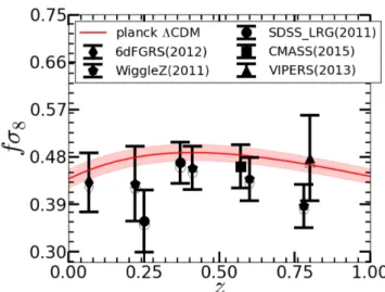
betweenz=0.06 and 0.8 listed in Table1as our main data points. Fig.1shows the measurements used with and without corrections andPlanck2013 prediction. We briefly describe each of the surveys andfσ8measurements in the following sections.

3.1 6dFGRS

The 6dFGRS (6 degree Field Galaxy Redshift Survey) has observed 125 000 galaxies in near-infrared band across 4/5th of southern sky (Jones et al.2009). The surveys covers redshift range 0< z <0.18, and has an effective volume equivalent to 2dFGRS (Percival et al.

2004) galaxy survey. The RSD measurement was obtained using a subsample of the survey consisting of 81 971 galaxies (Beutler et al.2012). The measurement offσ8was obtained by fitting 2D

correlation function using streaming model and fitting range 16–30 Mpch−1_{. The Alcock–Paczynski (AP) effect (Alcock & Paczynski}

1979) has been taken into account and it has a negligible effect (Beutler et al.2012). The final measurement usesWilkinson Mi-crowave Anisotropy Probe7 (WMAP7; Bennett et al.2013) likeli-hood in the analysis. To be able to use thisfσ8measurement, we

Figure 1. The measuredfσ8from different surveys covering redshift range 0.06< z <0.8. The empty markers represent the reported measurement of fσ8and the filled markers are for the corrected values forPlanckcosmology. The red band shows thePlanckCDM 1σprediction.

need to account for the transformation to thePlanckbest-fitting cosmology (Planck Collaboration I2014a).

3.2 2dFGRS

The 2dFGRS (2 degree Field Galaxy Redshift Survey) obtained spectra for 221 414 galaxies in visible band on the southern sky (Colless et al.2003). The survey covers redshift range 0< z <0.25 and has an effective area of 1500 square degrees. The RSD mea-surement was obtained by linearly modelling the observed distortion after splitting the overdensity into radial and angular components (Percival et al.2004). The parameters were fixed at different val-uesns=1.0,H0=72. The results were marginalized over power

spectrum amplitude andbσ8. We are not using this measurement

in our analysis for two reasons. First, the survey has a huge over-lap with 6dFGRS which will lead to a strong correlation between the two measurements. Secondly, the cosmology assumed is quite far fromWMAP7 andPlanckwhich may cause our linear theory approximation used to shift the cosmology to fail.

3.3 WiggleZ

The WiggleZ Dark Energy Survey is a large-scale galaxy redshift survey of bright emission line galaxies. It has obtained spectra for nearly 200 000 galaxies. The survey covers redshift range 0.2< z <

1.0, covering effective area of 800 square degrees of equatorial sky (Blake et al.2011b). The RSD measurement was obtained using a subsample of the survey consisting of 152 117 galaxies. The final result was obtained by fitting the power spectrum using the Jennings, Baugh & Pascoli (2011) model in four non-overlapping slices of redshift. The measured growth rate isfσ8(z)=(0.42±

0.07, 0.45±0.04, 0.43±0.04, 0.38±0.04) at effective redshift

z=(0.22, 0.41, 0.6, 0.78) with non-overlapping redshift slices of

zslice=([0.1, 0.3], [0.3, 0.5], [0.5, 0.7], [0.7, 0.9]), respectively. We

can assume the covariance between the different measurements to be zero because they have no volume overlap.

(5)

3.4 SDSS LRG

The Sloan Digital Sky Survey (SDSS) Data Release 7 (DR7) is a large-scale galaxy redshift survey of luminous red galaxies (LRGs; Eisenstein et al.2011). The DR7 has obtained spectra of 106 341 LRGs, covering 10 000 square degrees in redshift range 0.16< z <

0.44. The RSD measurement was obtained by modelling monopole and quadruple moment of galaxy auto-correlation function using linear theory. The data were divided in two redshift bins: 0.16< z <0.32 and 0.32< z <0.44. The measurements of growth rate are

fσ8(z)=(0.3512±0.0583, 0.4602±0.0378) at effective redshift

of 0.25 and 0.37, respectively (Samushia et al.2012). These mea-surements are independent because there is no overlapping volume between the two redshift slices.

3.5 BOSS CMASS

SDSS Baryon Oscillation Spectroscopic Survey (BOSS; Dawson et al.2013) targets high-redshift (0.4< z <0.7) galaxies using a set of colour–magnitude cuts. The growth rate measurement uses the CMASS (Reid et al.2016; Anderson et al.2014b) sample of galaxies from Data Release 11 (Alam et al.2015a). The CMASS sample has 690 826 LRGs covering 8498 square degrees in the redshift range 0.43< z <0.70, which correspond to an effective volume of 6 Gpc3_{. The}_f_σ

8is measured by modelling the monopole

and quadruple moment of galaxy auto-correlation using convolution Lagrangian perturbation theory (Carlson, Reid & White2013) in combination with Gaussian streaming model (Wang, Reid & White

2014). The reported measurement of growth rate isfσ8=0.462±

0.041 at effective redshift of 0.57 (Alam et al.2015b).

We are also using the combined measurement of growth rate (fσ8), angular diameter distance (DA) and Hubble constant (H)

measured from the galaxy auto-correlation in CMASS sample at an effective redshift of 0.57 (Alam et al.2015b). The measurement and its covariance are given below and it is called eCMASS,

f σ8=0.46, DA=1401, H =89.15

CeCMASS=

⎛ ⎜ ⎜ ⎜ ⎜ ⎜ ⎜ ⎝

0.0018 −0.6752 −0.1261

−0.6752 550.61 45.881

−0.1261 45.881 14.019

⎞ ⎟ ⎟ ⎟ ⎟ ⎟ ⎟ ⎠

. (8)

3.6 VIPERS

VIPERS (de la Torre et al.2013) is a high-redshift small-area galaxy redshift survey. It has obtained spectra for 55 358 galaxies covering 24 square degrees in the sky from redshift range 0.4< z <1.2. The measurement of growth factor uses 45 871 galaxies covering the redshift range 0.7< z <1.2. Thefσ8measurement is obtained by

modelling the monopole and quadruple moments of galaxy auto-correlation function between the scale 6 and 35h−1_{Mpc. They}

have reportedfσ8=0.47±0.08 at effective redshift of 0.8. The

perturbation theory used in the analysis has been tested against

N-body simulation and shown to work at mildly non-linear scale below 10h−1_{Mpc (de la Torre et al.}₂₀₁₃_).

3.7 PlanckCMB

Planckis a space mission dedicated to the measurement of CMB anisotropies. It is the third generation of all sky CMB experiment followingCOBEandWMAP. The primary aim of the mission is to measure the temperature and polarization anisotropies over the entire sky. ThePlanckmission provides a high-resolution map of

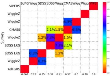
Figure 2. Correlation matrix between all the measurements used in our analysis. We have estimated the correlation as the fraction of overlap volume between two surveys to the total volume of the two surveys combined.

CMB anisotropy which is used to measure the cosmic variance-limited angular power spectrumCT T

at the last scattering surface.

ThePlanckmeasurements help us constrain the background cos-mology to unprecedented precision (Planck Collaboration I2014a; Planck Collaboration XVI2014c; Planck Collaboration2015a). We are using the CMB measurements fromPlancksatellite in order to constrain cosmology. We have assumed thatPlanckmeasurements are independent of the measurement of growth rate from various galaxy redshift surveys.

3.8 Correlation matrix

We use the measurements of fσ8 from six different surveys.

Although these surveys are largely independent, and in some cases they probe different biased tracers, they are measuring in-herently the same matter density field. Therefore, the parts of the survey observing the same volume of sky cannot be treated as in-dependent. We have predicted an upper limit to the overlap volume using the data from different surveys. We have estimated the frac-tional overlap volume between any two samples as the ratio of the overlap volume to the total volume of the two samples. We estimate the correlation between two measurements as the fractional overlap volume between the two measurements. Fig.2shows our estimate of the correlation between the surveys. The four measurements of WiggleZ survey cover the redshift range between 0.1 and 0.9 and hence show most correlation with other measurements like SDSS LRG and CMASS in the same redshift range.

4 P OT E N T I A L S Y S T E M AT I C S

The collection offσ8data points that we are using in this

analy-sis contains measurements from several different surveys, obtained during the last decade, each with a different pipeline. Furthermore, often the latter implicitly assumes a GR modelling, which does not take into account the different predictions for the growth factor in modified theories of gravity. It is important to account for some cru-cial differences in order to use these measurements in our analysis. We have looked at following different aspects of measurements and theoretical prediction before using them in our analysis.

(6)

4.1 Fiducial cosmology of the growth rate (fσ8)

The measurements offσ8have been obtained over the time when we

had transition fromWMAPbest-fitting cosmology (Hinshaw et al.

2013) to thePlanckbest-fitting cosmology (Planck Collaboration I

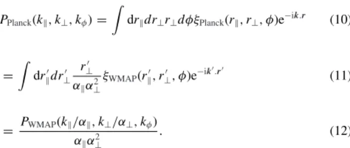
2014a). Since we are usingPlancklikelihood (Planck Collaboration XV2014b) in our analysis, we have decided to convert all the mea-surements toPlanckcosmology. The three-dimensional correlation function can be transformed fromWMAPto thePlanckcosmology using AP effect (Alcock & Paczynski1979),

ξPlanck(r, r⊥, φ)=ξWMAP(αr, α⊥r⊥, φ), (9)

where α is the ratio of the Hubble parameters (α=

HPlanck/HWMAP) andα⊥ is the ratio of the angular diameter dis-tances (α⊥=DAWMAP/DAPlanck). Ther,r⊥are pair separations along

the line of sight and perpendicular to the line of sight, andφis the angular position of pair separation vector in the plane perpendic-ular to the line of sight from a reference direction. In practice, the correlation function is isotropic alongφ. We can calculate the corresponding power spectrum by applying Fourier transform to correlation function,

PPlanck(k, k⊥, kφ)=

drdr⊥r⊥dφξPlanck(r, r⊥, φ)e−ik.r (10)

=

drdr_⊥ r

⊥

αα2

⊥

ξWMAP(r, r_⊥, φ)e−ik

_._r

(11)

= PWMAP(k/α, k⊥/α⊥, kφ)

αα2

⊥

. (12)

The Kaiser formula for RSD gives the redshift space correlation function as Ps

g(k, μ)=b 2_P

m(k)(1+βμ2)2(Kaiser1987). Using

the linear theory Kaiser prediction and the above approximation betweenWMAPandPlanckpower spectrum, we can get a relation to transform the growth function fromWMAPtoPlanckcosmology,

1+βPlanckμ2

1+βWMAPμ2 =C

PPlanck(k, μ)

PWMAP(k, μ)

(13)

=C

1

αα2

⊥

, (14)

whereCis the ratio of isotropic matter power spectrum withWMAP

and Planckcosmology integrated over scale used inβ measure-ment, C= k2 k1 dk Pm WMAP(k)

Pm Planck(k)

, (15)

with k(,⊥)=k(,⊥)/α(,⊥). When the right-hand side of

equa-tion (14) is close to 1, then we can approximate the above equaequa-tion as follows:

βPlanck=βWMAPC

μ2

1

αα2

⊥

. (16)

The ratio μ2

μ2 can be obtained using simple trigonometry which

gives following equations, where the last equation is approximation forα2

≈α2⊥,

μ2

μ2 =

1

α2

⊥

α2

+(α2⊥−α2)μ2

≈ α α⊥ 2 . (17)

We can substitute equation (17) in equation (16) in order to get the required scaling forf(growth factor) assuming that bias measured is proportional to theσ8of the cosmology used,

βPlanck=βWMAPC α α2 ⊥ (3/2) (18)

f σ_8Planck=f σ_8WMAPC

α

α2

⊥

(3/2)

σ8Planck

σWMAP 8

2

. (19)

We have tested prediction of equation (19) against the measure-ment offσ8reported in table 2 of Alam et al. (2015b) at redshift

0.57 using bothPlanckandWMAPcosmology. In principle, the bias in the measurements offσ8should be corrected for the each step of

MCMC to the chosen cosmology. But, we choose not to incorporate that and apply only an overall correction. Because the corrections are negligible compared to the error on measurements.

4.2 Scale dependence

GR predicts a scale-independent growth factor. One of the impor-tant features of the MG theories we are considering is that they predict a scale-dependent growth factor which has a transition from high to low growth at certain scale which depends on the redshift

zand the model parameters. The measurements we use from the different surveys assume a scale-independentfσ8and uses

charac-teristic length-scale while analysing data. In order to account for all these effects, we have done our analysis in two different ways. In the first method, we assume that the measurements correspond to an effectivekand in the second method, we treat the average theoretical prediction over range ofkused infσ8analysis.

Figs 11 and12 show the parameter constraint for Chameleon models andf(R) gravity. The grey and red contours result from using two different model predictions to test the scale dependence. The grey contours correspond to the model where we averagefσ8

overkused in respectivefσ8analysis and red contours correspond

tofσ8evaluated atk=0.2hMpc−1. It is evident from the plots that,

at the current level of uncertainty, we obtain very similar constraint and hence do not detect any significant effect of scale dependence offσ8.

4.3 Other systematics

The measurements offσ8are reported at the mean redshift of the

surveys. But the galaxies used have a redshift distribution which in principle can be taken into account by integrating the theoretical prediction. This should be a very small effect because thefσ8(z) is

relatively smooth and flat (see Fig.1and Huterer et al.2015) for the redshift range of the survey and also because the survey win-dow for every individual measurement is small. Another important point is the assumption of GR-based modelling for the measure-ment. We have looked at the modelling assumption for each of the measurements. All measurements offσ8except WiggleZ and

VIPERS allow the deviation from GR through AP effect (Alcock & Paczynski1979) which justifies our use ofMGmodels. The inclu-sion of AP in WiggleZ and VIPERS will marginally increase the error on the measurements. Different surveys use different ranges of scale in the RSD analysis. This will be important especially while analysingMGmodels. To account for the different scales used, we evaluate the prediction for each survey averaged over the scale used in the respective analysis.

(7)

5 A N A LY S I S

We have measurement offσ8from various surveys covering redshift

range 0.06–0.8 (see Table1). We first correct these measurements for the shift fromWMAPcosmology toPlanckcosmology as de-scribed in Section 4.1. The next step is to evaluate prediction from different MG theories by evolving a full set of linear perturbation equations. The theoretical predictions forfσ8are generally scale

and redshift dependent (see Section 4.2). Therefore, we consider two cases for theoretical prediction: (1) evaluatefσ8at effective

kand (2) evaluatefσ8averaged over range ofkused in

measure-ments. We also predictCT T

l for different MG theories. Finally, we

define our likelihood, which consists of three parts, one by matching

Plancktemperature fluctuationCT T

l , second by matching growth

factor from Table1and third by using eCMASS data as shown in equation (8). Therefore, we define the likelihood as follows:

L=LPlanckLf σ8LeCMASS (20)

Lf σ8=e

−χ2

f σ8/2 (21)

χf σ28=f σ8C

−1

f σ8T. (22)

Thefσ8is the deviation of the theoretical prediction from the

measurement andC−1_{is the inverse of covariance which has}

diago-nal error for different surveys and correlation between measurement as described in Section 3.8. Note that we do not includefσ8from

CMASS while using eCMASS withfσ8(z) to avoid double

count-ing. This likelihood is sampled using modified version ofCOSMOMC

(Lewis & Bridle2002; Hojjati et al.2011). We sample over 6 cos-mology parameters{bh2,ch2, 100MC,τ,ns, log(1010As)}and

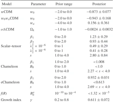
all 18Plancknuisance parameters as described in Planck Collab-oration I (2014a) with the respective extension parameters or MG parameters. The priors we have used on all the parameters are the same as the priors in Planck Collaboration I (2014a), and the priors we used on the parameters of MG model are given in Table2.

6 R E S U LT S

We have combined CMB data set and measurements of growth from various redshift surveys in order to constrain the parame-ters of standard cosmology (CDM), extended cosmology models andMG. Our analysis gives consistent constraints for the standard

CDM parameters{bh2,ch2, 100MC,τ,ns, log(1010As)}as

shown in Table3. Fig.3shows the constraint onm–σ8plane for

CDM,wCDM,oCDM, scalar–tensor model, Chameleon grav-ity, eChameleon,f(R) and growth index parametrization. These are our best constraints obtained usingPlanck+eCMASS+ fσ8(z).

Fig.4shows the theoretical predictions offσ8(z) for each of the

models considered in this paper.

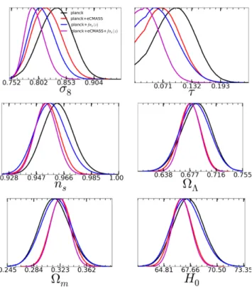
6.1 CDM

Fig.5shows the one-dimensional marginalized likelihood for stan-dardCDM cosmology. The black line shows the constraints from

Planck 2013 alone. The red, blue and magenta lines are pos-terior obtained for the data set combinationsPlanck+eCMASS,

Planck+fσ8(z) and Planck+eCMASS+fσ8(z), respectively. Our

parameter constraints are completely consistent with thePlanck

2013 results. Adding measurements of the growth rate toPlanck

Table 2. The list of extension parameters for all the models used in our analysis. For each parameter, we provide their symbol, prior range, central value and 1σerror.

Model Parameter Prior range Posterior

wCDM w0 −2.0 to 0.0 −0.873±0.077

w0waCDM w0 −2.0 to 0.0 −0.943±0.168 wa −4.0 to 4.0 0.156±0.361

oCDM k −1.0 to 1.0 −0.0024±0.0032

β1 0 to 2.0 1.23±0.29

β2 0 to 2.0 0.93±0.44

Scalar–tensor λ21×10−6 0 to 1 0.49±0.29 λ22×10−6 0 to 1 0.41±0.28

s 1.0 to 4.0 2.80±0.84

β1 1.0 to 2.0 <1.008

Chameleon B0 0 to 1.0 <1.0

s 1.0 to 4.0 2.27<s<4.0

β1 0 to 2.0 0.932±0.031

eChameleon B0 0 to 1.0 <0.613

s 1.0 to 4.0 2.69<s<4.0 f(R) Ba

0 10−10to 10−4 <1.32×10−5

Growth index γ 0.2 to 0.8 0.611±0.072

a_{We have tried using both logarithmic and linear prior on}_B

0 for thef(R) model and obtained similar results for the upper limit onB0. But, our final results are obtained using logarithmic prior onB0because the linear prior never converged due to huge range and strong constraint.

data does not improve the results (see Fig.5) due to already tight constraints fromPlanckobservations (see Fig.1).

6.2 DE equation of state (wCDM)

We have looked at thewCDM, i.e. the one-parameter extension of

CDM where the DE equation of state is a constant,w. Fig.6shows the two-dimensional likelihood ofw0andm. The grey contours

arePlanck-only constraint (w0= −1.27±0.42), red contours are

Planckand eCMASS (w0= −0.92±0.10) and blue contours show

Planckcombined with eCMASS and growth factor measurements (w0= −0.87±0.077). We obtainw0= −0.87±0.077 (8.8 per cent

measurement) which is consistent with the fiducial value ofw=

−1 forCDM. The constraint we obtained is similar in precision as compared to BAO only, but has different degeneracy. Therefore, combined measurement of growth rate and anisotropic BAO for all of these surveys will help us improve the precision ofw0.

6.3 Time-dependent DE (w0waCDM)

ThewCDM model which proposes a constant DE is limited in its physical characteristics. Many models propose time-dependent DE which is popularly tested using linear relationw(z)=w0+wa₁₊z_z,

withw0and waas free parameters. This model has been shown

to match exact solutions of distance, Hubble, growth to the 10−3

level of accuracy (de Putter & Linder2008) for a wide variety of scalar field (andMG) models. The dynamical evolution ofw(z) can change the growth factor significantly and leave an imprint on the CMB. The combination of CMB and collection of growth factor at different redshifts is a unique way to test the time-dependent DE model.

Fig.7shows the 1σ and 2σ region for (w0,wa). The grey

con-tour is from the Plancktemperature power spectrum data alone

(8)

Table 3. The list of standardCDM parameters used in our analysis. For each parameter, we provide its symbol, prior range, central value and 1σerror. We have used the same prior asPlanck2013 on these parameters. We have also marginalized over all the nuisance parameters ofPlancklikelihood. We report the results for each of the models analysed in this paper.

Models bh2 ch2 100θMC τ ns ln (1010As)

Prior range 0.005–0.10 0.001–0.99 0.50–10.0 0.01–0.8 0.9–1.1 2.7–4.0

CDM 0.0219±0.0002 0.1208±0.0020 1.0410±0.0006 0.0442±0.0236 0.953±0.0068 3.0007±0.0450 wCDM 0.0221±0.0003 0.1183±0.0028 1.0414±0.0006 0.0911±0.0449 0.9615±0.0097 3.0884±0.0843 w0waCDM 0.0221±0.0003 0.1181±0.0029 1.0415±0.0007 0.0906±0.0454 0.9619±0.0099 3.0871±0.0850

oCDM 0.0220±0.0003 0.1191±0.0031 1.0413±0.0007 0.0518±0.0278 0.9582±0.0094 3.0118±0.0514 Scalar–tensor 0.0221±0.0003 0.1199±0.0020 1.0412±0.0006 0.0333±0.0198 0.9591±0.0071 2.9769±0.0377 Chameleon 0.0219±0.0002 0.1205±0.0020 1.0411±0.0006 0.0390±0.0222 0.9539±0.0067 2.9894±0.0425 eChameleon 0.0218±0.0003 0.1222±0.0023 1.0409±0.0006 0.1313±0.0467 0.9537±0.0079 3.1780±0.0914 f(R) 0.0221±0.0004 0.1182±0.0033 1.0414±0.0008 0.0733±0.0354 0.9607±0.0101 3.0526±0.0663 Growth index (γ) 0.0218±0.0003 0.1214±0.0023 1.0409±0.0006 0.0699±0.0400 0.9525±0.0075 3.0534±0.0788

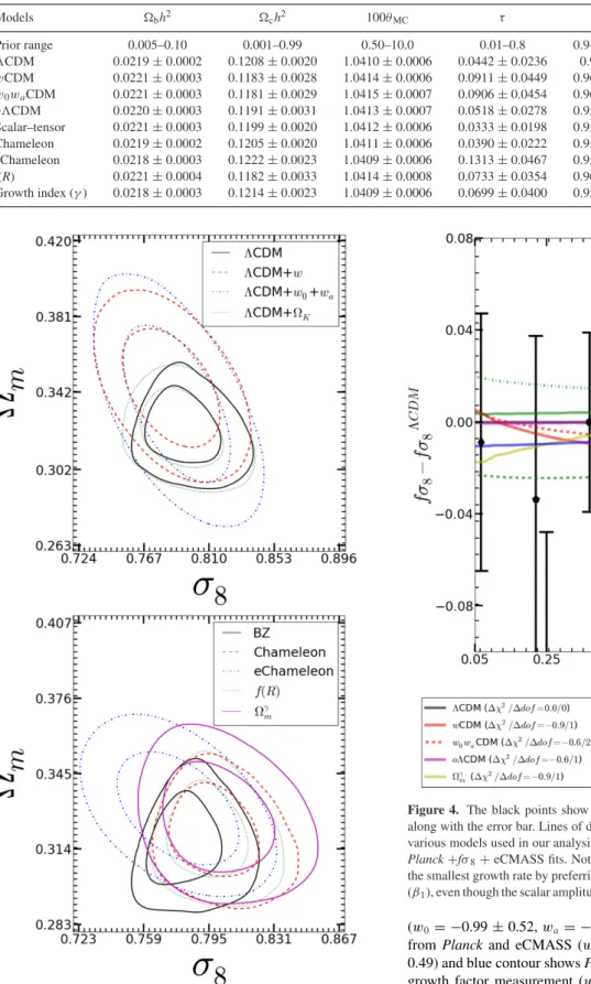
Figure 3. The 1σand 2σregions for each of the models considered in this paper in them–σ8plane. It shows that the posterior likelihood is consistent for each of the models in this parameter space. The top plot shows the models which are extension toCDM and the bottom plot shows theMGmodels.

Figure 4. The black points show the correctedfσ8used in our analysis, along with the error bar. Lines of different colours show the best fit for the various models used in our analysis. The best fit andχ2_{are for the case of} Planck+fσ8+eCMASS fits. Notice that the eChameleon model predicts the smallest growth rate by preferring lower values of the coupling constant (β1), even though the scalar amplitude of primordial power spectrum is high.

(w0= −0.99±0.52,wa= −1.50±1.46). The red contours are

fromPlanck and eCMASS (w0= −1.23± 0.26,wa =0.63±

0.49) and blue contour showsPlanckcombined with eCMASS and growth factor measurement (w0= −0.94±0.17,wa =0.16±

0.36). TheCDM prediction of (w0,wa)=(−1, 0) is completely

consistent with our posterior. We have obtained constraint on

w0= −0.94±0.17 (18 per cent measurement) and 1+wa=1.16 ±0.36 (31 per cent measurement) which is stronger constraint than

(9)

Figure 5. CDM: we use GR as the model for gravity to determine the growth factor and fit forfσ8(z) and eCMASS measurement withPlanck likelihood. The black line shows the constraints fromPlanck2013 alone. The red, blue and magenta lines are posterior obtained for the data set combi-nationsPlanck+eCMASS,Planck+fσ8(z) andPlanck+eCMASS+fσ8(z), respectively. The two most prominent effects are in optical depthτ and scalar amplitude of primordial power spectrumAs, which is also reflected in the derived parameterσ8and mid-redshift of reionizationzre.

Figure 6. wCDM: the two-dimensional posterior likelihoodwandmfor wCDM. The grey contour is forPlanck(w0= −1.27±0.42); red contour is combined constraint fromPlanckand eCMASS (w0= −0.92±0.10). The blue contour represents constraint from combiningPlanckwith eCMASS andfσ8(z) (w0= −0.87±0.077).

Figure 7. w0waCDM: the two-dimensional posterior likelihood ofw0and wa for time-dependent DE model. The grey contour is forPlanck(w0=

−0.99±0.52,wa = −1.50±1.46); red contour is combined constraint

fromPlanckand eCMASS (w0= −1.23±0.26,wa=0.63±0.49). The

blue contour represents results from combiningPlanckwith eCMASS and fσ8(z) (w0= −0.94±0.17,wa=0.16±0.36).

the current best measurement ofwa= −0.2±0.4 from Aubourg

et al. (2015).

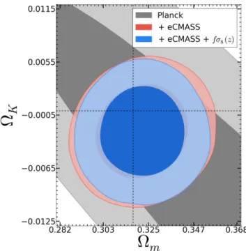
6.4 Spatial curvature (oCDM)

We consider a model with spatial curvature parametrized withK

as free parameter calledoCDM along withCDM parameters. Fig.8shows the posterior for theKandmplane. The grey contour

is from thePlancktemperature power spectrum data alone (k= −0.060±0.047). The red contours are fromPlanckand eCMASS (k= −0.0024±0.0034) and blue contour showsPlanckcombined

with eCMASS and growth factor measurements (k= −0.0024±

0.0032). TheCDM prediction ofk=0 is completely

consis-tent with our posterior. We have obtained constraint on 1+k=

0.9976±0.0032 (0.3 per cent measurement) which is competitive with the current best measurements (Aubourg et al.2015). It will be interesting to see if combined RSD and BAO at all redshifts will give any improvement on the precision of curvature.

6.5 Scalar–tensor gravity (BZ parametrization)

The general scalar–tensor theories of gravity are analysed using five-parameter model called BZ parametrization. The five five-parameters of scalar–tensor gravity (β1,β2,λ1,λ2,s) are constrained along with

the standardCDM parameters usingPlanck,fσ8(z) and eCMASS

measurements. BZ model predicts a scale-dependent growth rate (fσ8(k,z)), whereas the measurements are at some effectivek. In

order to incorporate thek-dependence in our analysis, we use the two different approaches described in Section 4.2. Fig.9shows two-dimensional posterior in the plane (β1,β2). The green contour is

combined constraint fromPlanckand eCMASS (β1=1.18±0.29,

β2=0.95±0.43). The grey contour is the combined constraint

fromPlanckandfσ8(z) with averaged overk(β1= 1.24± 0.3,

(10)

Figure 8. oCDM: the two-dimensional posterior likelihood ofkand

mforoCDM. The grey contour is forPlanck(k= −0.060±0.047);

red contour is combined constraint from Planck and eCMASS (k = −0.0024±0.0034). The blue contour represents results from combining Planckwith eCMASS andfσ8(z) (k= −0.0024±0.0032).

Figure 9. BZ: the two-dimensional posterior likelihood ofβ1–β2for five-parameter scalar–tensor theory parametrized through the BZ form of equa-tion (2). The green contour is the combined constraint fromPlanckand eCMASS (β1 =1.18±0.29,β2 = 0.95± 0.43). The grey contour is the combined constraint fromPlanckandfσ8(z) with averaged overk(β1

= 1.24 ± 0.3,β2 = 0.96 ± 0.45); red contour is the combined con-straint fromPlanckandfσ8(z) at effectivek=0.2hMpc−1(β1=1.24

±0.3,β2 =0.95±0.45). The blue contour represents results from the combination of Planck, fσ8(z) and eCMASS (β1 = 1.23 ± 0.29, β2=0.93±0.44).

β2=0.96±0.45); the red contour is the combined constraint from

Planckandfσ8(z) at effectivek=0.2hMpc−1(β1=1.24±0.3,

β2= 0.95±0.45). The blue contour represents results from the

combination ofPlanck,fσ8(z) and eCMASS (β1=1.23±0.29,β2 =0.93±0.44). We obtain the following joint constraint on the five BZ parameters:β1=1.23±0.29,β2=0.93±0.44,λ21(×10−6)=

0.49±0.29,λ2 2(×10−

6₎₌₀_.₄₁_±₀_._{28 and}_s₌_2.80_±_{0.84. By}

looking at the joint 2D likelihood for (β1,β2) in Fig.9, we notice

that there is a strong degeneracy between the two parameters which reflects the degeneracy betweenμandγfor the observables that we are using. Similar results have been found in Hojjati et al. (2012) and Planck Collaboration (2015b). For the next models that we will discuss,β1andβ2are not independent and this will allow data to

place more stringent constraints.

While the constraints on the length-scale of the scalar field (λ1,

λ2) and (s) are very broad, the one on the coupling,β1andβ2, is the

first ever constraint obtained on these parameters for general scalar– tensor gravity. The discrepancy in the strength of the constraints on the coupling and on the length-scale can be linked to the fact that data strongly prefer values of the coupling constants close to 1. For such values, the scale and time dependences in (μ,γ) become less important and therefore are loosely constrained. We will encounter this again in the Chameleon andf(R) gravity cases.

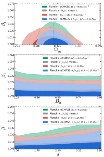
6.6 Chameleon gravity

The three parameters of Chameleon gravity (β1, B0, s) are

con-strained along with the standardCDM parameters usingPlanck,

fσ8(z) and eCMASS measurements. Chameleon models predict a

scale-dependent growth rate (fσ8(k,z)), whereas the measurements

are at some effectivek. In order to incorporate thek-dependence in our analysis, we use the two different approaches described in Section 4.2. Fig.10 shows the two-dimensional posterior in the plane (m,β1), (B0,β1) and (s,β1). The grey and red contours

show the posteriors from combined data set ofPlanckand growth rate measurements. The red contours are likelihood while eval-uating the growth rate at an effective k (β1 < 1.010), whereas

grey contours are for the case when we use an effective growth rate, averaged over the scales used in the actualfσ8measurement

(β1<1.010). The green contour is combined constraint fromPlanck

and eCMASS (β1< 1.013). Finally, the blue contours show the

posterior from combined data ofPlanck, eCMASS and growth rate (β1<1.008). We obtain the following joint constraint on the three

Chameleon parameters:β1<1.008,B0<1.0 and 2.27<s<4.

While the constraints on the length-scale of the scalar field,B0and

sare very broad, the one on the coupling,β1, is very strong and

predictsβ1= 1 to 0.8 per cent, bringingμto its GR value. As

we already discussed for the scalar–tensor case, the discrepancy in the strength of these constraints is due to the fact that data prefer values of the coupling constant close to 1, for which the time and scale dependences of (μ,γslip) become negligible. This is even more

the case for Chameleon models, where the theoretical prior forces

β1> 1, which corresponds to enhanced growth, and data

conse-quently require very small values for this coupling, pushingμvery close to its GR value.

We have also looked at the extended Chameleon model where we allowβ1to be less than 1 following previous analysis of this model.

Fig.11shows the two-dimensional posterior in the plane (m,β1).

The red contours are likelihood while evaluating the growth rate at an effectivek(β1=0.940±0.032), whereas grey contours are for

the case when we use an effective growth rate, averaged over the scales used in the actualfσ8measurement (β1=0.936±0.032).

(11)

Figure 10. Chameleon theory: the two-dimensional posterior likelihood for Chameleon gravity. The green contour is the combined constraint from Planckand eCMASS (β1 < 1.013). The grey contour is the combined constraint fromPlanckandfσ8(z) with averaged overk(β1<1.010); the red contour is the combined constraint fromPlanckandfσ8(z) at effective k=0.2hMpc−1(β1<1.010). The blue contour represents results from the combination ofPlanck, eCMASS andfσ8(z) (β1<1.008).

The green contour is combined constraint fromPlanck and eC-MASS (β1=0.932±0.04). Finally, the blue contours show the

posterior from combined data ofPlanck, eCMASS and growth rate (β1=0.932±0.031). We obtain the following joint constraint on

the three eChameleon parameters:β1=0.932±0.031,B0<0.613

and 2.69< s< 4. Like in the more general scalar–tensor case, while the constraints on the length-scale of the scalar field,B0and

sare very broad, the one on the coupling,β1, is a huge

improve-ment on the previous constraint ofβ1=1.3±0.25 (19.2 per cent

measurement) usingWMAPCMB, SNe and ISW data set (Hojjati et al.2011). Let us notice that when we constrain jointly the three eChameleon parameters, data select a region in the parameter space which corresponds toβ1<1, i.e. to suppressed growth. This region

excludes standard Chameleon models, includingf(R) theories, for whichβ1>1 and the growth is enhanced. After all, as we have

seen above and will see in the next section, the same data place very stringent constraints on Chameleon andf(R) models, forcing them to be very close toCDM (see Figs11and12). Hence, the combination of data sets that we employ favours models with a suppressed growth rate, which adopting the BZ parametrization can be obtained withβ1<1; a suppressed growth was favoured also

Figure 11. eChameleon theory: the two-dimensional posterior likelihood ofβ1andmfor extended Chameleon gravity. The green contour is the combined constraint fromPlanckand eCMASS (β1=0.932±0.04). The grey contour is the combined constraint fromPlanckandfσ8(z) with aver-aged overk(β1=0.940±0.032); red contour is combined constraint from Planckandfσ8(z) at effectivek=0.2hMpc−1(β1=0.936±0.032). The blue contour represents results from the combination ofPlanck,fσ8(z) and eCMASS (β1=0.932±0.031).

Figure 12. f(R) gravity: the two-dimensional posterior likelihood ofB0and mforf(R) gravity. The green contour is combined constraint fromPlanck and eCMASS (B0 < 3.43× 10−5). The grey contour is the combined constraint fromPlanckandfσ8(z) with averaged over k(B0 <2.77× 10−5); the red contour is the combined constraint fromPlanckandfσ8(z) at effectivek=0.2hMpc−1_(B

0<1.89×10−5). The blue contour represents results from the combination ofPlanck,fσ8(z) and eCMASS (B0<1.36× 10−5_).

(12)

by the data set used in Planck Collaboration (2015b), although in that case the authors employed a time-dependent parametrization. Theoretically viable scalar–tensor models with a suppressed growth are discussed in Perenon et al. (2015), where they are analysed via a scale-independent parametrization in the effective field theory language.

6.7 f(R) theory

We consider one-parameter (B0) model of f(R) gravity. The

pa-rameter B0 parametrizes the deviation from CDM. The model

approaches GR whenB0is zero. Similar to Chameleon theory,f(R)

gravity predicts a scale-dependent growth rate (fσ8(k,z)). Fig.12

shows the two-dimensional posterior inB0andmplane. The green

contour is combined constraint fromPlanckand eCMASS (B0<

3.43×10−5_{). The grey and red contours show posterior from}

com-bined data set ofPlanckand growth rate measurements. The red contours are likelihood while evaluating the growth rate at an effec-tivek(B0<1.89×10−5), whereas grey contours are for the case

when we use effective growth rate, which is averaged over scales used in the actualfσ8measurements (B0<2.77×10−5). The blue

contours show the posterior from combined data of Planck, eC-MASS and growth rate (B0 <1.36×10−5). We obtainedB0 <

1.36×10−5₍₁_σ _{C.L.), which is an improvement by a factor of}

4 on the most recent constraint from large-scale structure ofB0=

5.7×10−5₍₁_σ_{C.L.; Xu}₂₀₁₅_{). Our constraint is competitive with}

the constraint from Solar system tests and clusters (Hu & Sawicki

2007; Schmidt, Vikhlinin & Hu2009; Cataneo et al.2015).

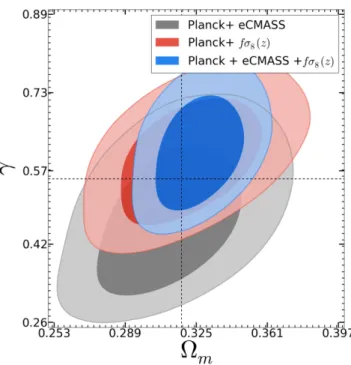
6.8 Growth index (γ) parametrization

The standard cosmological model, based on GR, predicts a precise value for the growth factor in the linear regime, i.e.f =0.55

m . In

order to test deviations from GR, we have parametrized the growth factor using growth indexγ(Linder & Cahn2008) asf =γ

m. The

marginalized two-dimensional likelihood form andγ is shown

in Fig.13. The grey contour is combined constraint fromPlanck

and eCMASS (γ = 0.477± 0.096). The red contours show the constraint obtained using Planckand fσ8(z) measurement (γ =

0.595 ±0.079) and the blue contours are for combined data set of Planck withfσ8(z) and eCMASS (γ = 0.612 ± 0.072). We

have obtainedγ = 0.612 ± 0.072 (11.7 per cent measurement) completely consistent with the GR prediction.

7 D I S C U S S I O N

We have constrained the parameters of the standard cosmological model,CDM, as well as those of various extensions using the cur-rent measurements of growth rate between redshift 0.06 and 0.83 (Fig.4), eCMASS andPlanck2013. We have been careful with sev-eral important details while combining results from various surveys and different cosmologies of measurements. We have first showed that the standardCDM parameter space has a consistent posterior, independent of the model considered except for Chameleon grav-ity. Next, we focused on each model and analysed the constraint on its extension parameters. As for the standard model,CDM, using the growth factor we do not improve constraints on any of its parameters because the growth rate is already highly constrained withPlanckmeasurement for the standard model of cosmology. It is impressive to notice thatCDM, without any extra parameter, is completely consistent with the measurements offσ8from very

different galaxy types and redshifts. In the case of the extension

Figure 13. Growth index (γ): the two-dimensional posterior likelihood ofγ andmfor growth index parametrization. The grey contour is the combined constraint fromPlanckand eCMASS (γ=0.477±0.096). The red contour is the combined constraint fromPlanckandfσ8(z) (γ=0.595±0.079). The blue contour represents results from the combination ofPlanck,fσ8(z) and eCMASS (γ=0.612±0.072).

where the DE equation of state is constant but free to vary,wCDM, we obtainw0= −0.87±0.077 (8.8 per cent measurement). This is

a 3.7 times improvement on the precision compared toPlanck-only measurementw= −1.27±0.42 (33 per cent measurement) and comparable to the 8 per cent measurement of Samushia et al. (2012). Our measurement prefersw <−1 at the 1σ level. We have also noticed that the growth rate and BAO have slightly different degen-eracy forwCDM. This shows the potential to improve the constraint onwby combining the growth rate and BAO measurements from a range of galaxy redshift surveys. However, one difficulty in doing so is to model the correlation between the measurement of growth rate and BAO.

We also report one of the best measurements on the parameters of the model with a time-dependent equation of state,w0waCDM. We

have measuredw0= −0.94±0.17 (18 per cent measurement) and

1+wa=1.16±0.36 (31 per cent measurement). This represents a

significant improvement onwacompared to all other measurements

(Aubourg et al.2015; Planck Collaboration I2014a). The measure-ments offσ8, H and DA in eCMASS help to constrain CDM

parameters, while the evolution of the growth rate over a large red-shift range, obtained through measurements offσ8(z) at multiple

redshifts, improves the constraint on evolving DE. This hints at the potential of using combined growth rate and anisotropic BAO as a function of redshifts, when future surveys like eBOSS andEuclid

(Laureijs et al.2011) will provide much stronger growth rate and BAO constraints at much higher redshifts. We have also looked at the possibility of a non-zero curvature for the universe,oCDM, finding 1+ k =0.9976±0.0032 (0.3 per cent measurement),

which is the same as the best constraint reported in Samushia et al. (2012). We notice that the optical depth (τ) and amplitude of scalar power spectrum (As) are relatively low foroCDM, which predicts

smaller redshift of reionization (zre=7.20±2.81) but is above the