Quantum-assisted Finite-element Design Optimization
Dyon van Vreumingen1, 3 , Florian Neukart1, 3, *, David Von Dollen1 , Carsten Othmer2, Michael Hartmann2, Arne-Christian Voigt2, and Thomas B¨ack3
1Volkswagen Group Region Americas, USA
2Volkswagen Group Research, Germany
3Leiden Institute for Advanced Computer Science, Leiden University, The Netherlands
*Corresponding author: Florian Neukart ([email protected])
August 13, 2019
Abstract
Quantum annealing devices such as the ones produced by D-Wave systems are typically used for solving optimization and sampling tasks [1–15], and in both academia and industry the characterization of their usefulness is subject to active research. Any problem that can naturally be described as a weighted, undirected graph may be a particularly interesting candidate [16,17], since such a problem may be formulated a as quadratic unconstrained binary optimization (QUBO) instance, which is solvable on D-Wave’s Chimera graph architecture.
In this paper, we introduce a quantum-assisted finite-element method for design optimization. We show that we can minimize a shape-specific quantity, in our case a ray approximation of sound pressure at a specific position around an object, by manipulating the shape of this object. Our algorithm belongs to the class of quantum-assisted algorithms, as the optimization task runs iteratively on a D-Wave 2000Q quantum processing unit (QPU), whereby the evaluation and interpretation of the results happens classically. Our first and foremost aim is to explain how to represent and solve parts of these problems with the help of a QPU, and not to prove supremacy over existing classical finite-element algorithms for design optimization.
Keywords: quantum computing, quantum physics, finite-element, design optimization, QUBO
1
Introduction
According to the laws of quantum mechanics, a quantum mechanical system, which
is in the ground state (state of minimal energy) of a time-independent system, also remains in the ground state if a change to it happens only slowly, i.e. adiabatically.
This is known as the adiabatic theorem. The idea of adiabatic quantum computing
is to construct a system having a ground state that is still unknown at that time, which corresponds to solving a particular problem, and another one whose ground
state is easy to prepare experimentally. Subsequently, the easy-to-prepare system
is adiabatically transferred to the system whose ground state one is interested in, and then measured. If the transition is slow enough, one can obtain a
minimum-energy solution to the problem. D-Wave’s QPUs deploy a system described by the
two-dimensional Ising spin hamiltonian [16, 17]:
Hh,J(s) =
n
X
i=1 hisi+
X
hi,ji
Jijsisj. (1)
Here,s is a vector of nspins, si∈ {−1,1}, which carry an individual energy weight
hi and are interconnected through 2-local couplingsJij. The sum in the second
term of the hamiltonian runs over only those spin pairs which are connected, as
Jij = 0 for uncoupled spin pairs. As such, the hamiltonian is characterised by the
linear weight vectorh and the coupling matrix J. The search for the minimum spin configurationsmin for the Ising hamiltonian is known to be NP-hard [15, 18].
It is generally preferable for a computational application to work with {0,1}
-valued bits of information as opposed to spins, which can be achieved through the
transformation xi = 12(si+ 1). This formulation of the Ising spin problem, which is
polynomially reducible to the original form and vice versa, is known as aquadratic
unconstrained binary optimization problem, or QUBO for short, and can be solved
by the QPU in the same fashion as a conventional Ising model. The equivalence between the two problem classes implies that any problem to be solved with the
D-Wave QPU may be formulated either as a QUBO instance or directly as an Ising model. The objective quantity that the QPU minimizes in the QUBO case is given
by the quadratic form [16, 17]
ObjQ(x) =x>Qx, (2)
wherexis anN-sized vector of{0,1}-valued variables, and Q is anN×N real-valued upper triangular matrix containing the (adjusted) linear weights in the diagonal,
and the couplings in the off-diagonal entries.
representing the binary variables, are the nodes, and the couplings the edges. The
initial configuration is set up such that all qubits are in uniform superposition,
|xii= √12(|0i+|1i). During the annealing cycle, the state is evolved according to
the energy landscape described by Q. Eventually, when the system reaches the
ground state, a minimum solution to the QUBO problem is found.
In this work, we demonstrate a method for using the QPU as an optimizer for a
finite-element design problem. That is, we seek to optimize the shape of a 3D body
defined by a finite number of elements against certain physical circumstances, by expressing the physical interaction of the elements in a QUBO form, and having
the QPU find the minimum-energy configuration corresponding to a (sub)optimal
shape. The next sections describe and discuss the problem in the framework of finite-element methods, as well as our approach to the problem and the observed
results.
This paper is structured as follows. Sections 2 and 3 briefly discuss the research field of finite-element methods, the problem we address and its context in vehicle
engineering, and how the two relate in our work. Section 4 outlines our method for
solving the problem, including a detailed description of the QUBO formulation and the procedure that our proposed algorithm follows. Section 5 showcases the results
in terms of shape optimization that we obtained by executing the algorithm, and
examines a number of features and limitations of the algorithm that appear from these results. Lastly, we present our conclusions in section 6 and give an outlook on
possible future work in section 7.
2
Finite-element methods
Finite-element methods (FEM) are a general group of numerical methods used
in various physical tasks. Most well-known is the application of FEM in the investigation of the strength and deformation of solids with a geometrically complex
shape, because here the use of classical methods, e.g. beam theory, proves to be
too time-consuming or impossible. Logically, the FEM is based on the numerical solution of a complex system of differential equations. The computation domain,
e.g. the solid, is divided into finitely many subdivisions of a simple form, creating
a mesh of the original solid using a finite number of corner points (‘vertices’) and faces (‘elements’ or ‘simplices’). The physical behaviour of this meshed solid can be
more easily calculated with well-known elementary functions due to its simplified
geometry. The physical behaviour of the whole body is modelled in the transition from one element to the next, through very specific problem-dependent continuity
certain point in the component at a given time. The search for the motion function is
thus returned to the search for the values functions’ parameters. By using more and more parameters such as more and/or smaller elements and higher order functions,
the accuracy of the approximate solution can be improved. The development of
the FEM was possible in essential stages only by the development of powerful computers, since it requires considerable computing power. Therefore, this method
was formulated from the outset to be processed on computers. Further information
can be found in the work by Pepper et al. [19].
3
Quantum-assisted finite-element method for design
optimization
With the algorithm we introduce in the following sections, we are able to find designs
based on a quantity that we minimize. One practical example concerns minimizing
the wind noises on an external mirror of a vehicle, and another one is minimizing the noises through vibrations caused by the engine or different road conditions in
a vehicle. The areas to optimize are commonly obtained with a complex
finite-element simulation, and evolutionary algorithms have proven to be very valuable for searching the design space [20–23]. As one part of the wind noise prediction
simulation chain, we can compute acoustic sources on the mirror surface. This is an
instance of a so-called acoustic scattering problem, which has to be solved in order to extract only those sources which are most relevant (noise-causing) at the position
of the passengers. Solving the scattering problem is very time-consuming, especially
in real vehicle applications, where the number of elements can be in the order
of millions. Even for relatively few, a direct solver implementing straightforward
matrix inversion quickly runs into memory and computation time limits. Thus, we are after finding an algorithm that scales better with an increasing number of
elements. The present state of quantum computing does not allow us to compete
with classical algorithms in terms of number of elements or speed, as the currently newest version of the QPU, containing approximately 2048 qubits, can only reliably
find minor embeddings for shapes with up to 50 elements. Of course, we can split a
QUBO instance with more than 50 elements and process problems of arbitrary size, but this significantly increases the required computation time.
In the introduced algorithm, we start with an initial shape and intend to find
a shape that deflects sound waves emitted by an acoustic monopole source such that the sound pressure within an area at another position around the shape is
minimized. In the same instance, our algorithm must be form-preserving, as in the
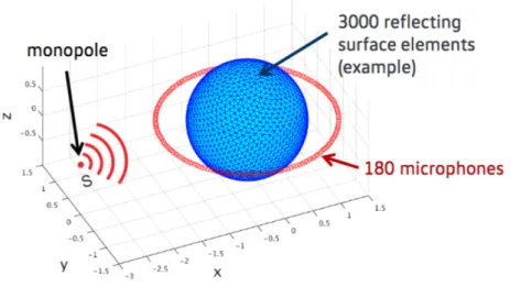
end the shape should still resemble the initial design. In the scenario we describe, the initial shape is a spherical mesh with finitely many triangular surface elements
(simplices), which is hit by sound waves emitted from an acoustic monopole (see
fig. 1). Fig. 1 shows microphones positioned around the shape, and the objec-tive is to minimize the sound pressure at any position of choice, by altering the
sphere’s shape. As the size of the current D-Wave QPU is limited to 2048 qubits
and each qubit bears only 6 connections to neighboring qubits, we make a num-ber of assumptions and approximations in order to make this problem feasible
for submission to the QPU with a reasonable number of elements. More
com-plex formulations however are possible, but adding more interactions would require more qubits, allowing processing of fewer elements within reasonable execution time.
4
Approach
In the definition of the sound scattering problem, we make one major simplification
to ensure that the resulting formulation is a finite-element method that is
well-suited for the QPU, which is to approximate sound waves as rays (i.e. straight lines in 3D space). That is, propagation of sound waves is treated similarly to
the propagation of light as done in graphical raytracing [24, 25], ignoring wave
effects and interference altogether. The most important reason for this is that it allows us to consider each element separately in terms of its contribution to
the measured sound pressure, as it avoids the necessity to construct a wave-based
a highly complex situation that cannot be described without distant (i.e.
non-neighbouring) element-element coupling. Since we seek to devise a QPU-assisted finite-element method for optimising a shape, finding a way to describe a ‘first-order
approximation’ with only neighbour couplings is more important than figuring out a
very accurate scattering solution. Since we know that sound waves in reality reflect linearly off a surface identically to light rays, we use this as the approximation to
base our quantum-assisted algorithm on.
The algorithm is a 3D search routine, which iteratively considers different candidate positions for each vertex in the shape (not to be confused with a qubit node
in the QPU graph), and then lets the QPU decide which vertex arrangement causes
the least number of rays to be reflected towards a microphone. This microphone is represented by a rectangularly bounded plane positioned next to the shape (see fig.
2). In each iteration, the routine assigns to each vertexK ‘mutations’, which are
small random deviations from the original vertex position; that is, for each vertex
vi in the set V of vertices, it considers vi+ dvi1,· · ·,vi+ dviK with dvij small. Each vertex is encoded by K qubits, and the |1i state of thej-th corresponding
qubit indicates that mutationj was assigned to this vertex (if the state is|0i, this particular mutation was not assigned). For each simplex, the partial loss `, being
the amount of pressure received from this simplex, is computed separately for each
of the K3 simplex configurations created from the vertex mutations (i.e. three vertices per simplex, andK mutations for each vertex). The QUBO matrix Q is
then constructed so that it contains, for each vertex, the loss information associated
with the simplices neighbouring the vertex. Based on this information, the QPU will choose the minimal loss vertex configuration among the ones supplied, and
use these as the input for the next iteration. This continues for a given number of iterations, or until convergence is observed.
A more detailed description of the QUBO formulation is provided in the next
section.
4.1 QUBO problem formulation
DefineS as the set of all simplicessdetermining the shape, N =|V|andC as the
set of all configurations c over the entire shape, wherec is a list of vertex mutation
assignments{(i, j)}, withi∈ {1, . . . , N}andj∈ {1, . . . , K}, indicating assignment of mutationj to vertexi(i.e. vi 7→vi+ dvij). Each configuration is a complete list, in that every vertex is assigned a mutation. Define a loss function L(S, c), which
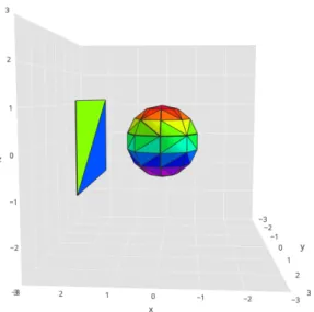
Figure 2. A rigid sphere, which serves as the initial shape, and a rectangular area at which the sound pressure must be minimized. The mere purpose of the colour scheme is visual aid.
simplicess∈S for configuration c,
L(S, c) =X
s∈S
`(s, c), (3)
and a loss partition functionZ(S, C), the sum of the loss function over all
configu-rations:
Z(S, C) =X
c∈C
L(S, c) =X
c∈C
X
s∈S
`(s, c). (4)
In this form, Z is a function of KN configurations. Now, we observe that this sum can be rewritten by visiting all edges (v,w) in the edge setE, and considering for each edge the two simplices adjacent to that edge. Since each simplex has three
edges, this means each simplex is counted thrice, so we divide this new total by 3,
to obtain:
Z(S, C) = 1 3
X
c∈C
X
(v,w)∈E
X
s∈S(v,w)
`(s, c), (5)
where S(v,w) is the set of the two simplices adjacent to edge (v,w).
configurations that are nonequivalent with respect to this simplex to sum over
(represented by the set Cs), and multiply the result byKN−3:
Z(S, C) = K
N−3
3
X
(v,w)∈E
X
s∈S(v,w)
X
c∈Cs
`(s, c). (6)
This representation of the partition function now gives us an intuitive way to define a QUBO matrix Q for this problem. This instance is to be minimized by a{0,1}
-valued vectorxrepresenting a configurationc(x), whose entry corresponding to the mutation assignment (i, j) is 1 ifvi is assigned mutationjand 0 otherwise, as stated before. That is, we view each entryxij as representing whether mutation (i, j) is
included in the configuration list ofc(x) (in which casexij = 1) or not (implying
xij = 0). The edge pairs naturally correspond to the off-diagonal terms of this
matrix: for any edge pair (vi1,vi2) with mutations (i
1, j1) and (i2, j2) respectively,
we only need to sum over the partial loss values for all possible configurations
regarding the two neighbouring simplices. If we define ˆ`(s, j1, j2, k) to be the partial loss from a simplex s adjacent to edge (vi1,vi2) (that is, s ∈S
(vi1,vi2)) when its
third, off-edge vertex is assigned mutation k(whilevi1 is assigned mutation j1 and
vi2 is assigned mutationj2), we thus obtain the following matrix form:
Qi1j1
i2j2 =α
X
s∈S
(vi1,vi2 )
K
X
k=1
ˆ
`(s, j1, j2, k). (7)
Here, α is an energy scaling factor that absorbs theKN−3/3 in front of the sum in eq. 7 (in practice, thisKN−3 will turn out to be huge, so adjustment is necessary). In this form of Q, each entry fixes an edge, and a configuration for both vertices
of this edge. Since Q contains K rows and K columns for each vertex, it is an
N K×N K matrix.
Lastly, it is important to make sure the QPU returns a result vectorxsuch that each vertex is being assigned only one mutation in the corresponding configuration
c(x). Since x is binary, this is equivalent to requiring
∀i: 0 =
K X
j=1
xij−1
2
=−
K
X
j=1
xij+ 2 K
X
j=1
K
X
j0>j
xijxij0 + 1. (8)
A straightforward way to enforce this requirement is by adding it as a penalty term
recent paper on QPU traffic flow optimization [15]:
˜
L(S,x) =L(S, c(x)) +λX
i
K X
j=1
xij−1
2
. (9)
In the QUBO matrix, this directly translates to adding−λto the diagonal elements
Qijij and adding 2λ to the off-diagonal elements Qijij0 (j0 > j) corresponding to
vertex vi. Provided λ is large enough, this measure guarantees the QPU sets exactly one of the bits xi1, . . . , xiK to 1, as any infeasible assignment would cause
an increase in loss that would be higher than any possible gain from selecting a
different configuration.
4.2 Algorithm
With an overview of the procedure in our approach, and an explanation of the QUBO formulation, we can now turn to the algorithm itself. This iterative algorithm
executes the following steps.
1. First, we generate the low-resolution mesh of an initial spherical shape. The
vertices of this shape are conveniently represented as rectangular lattice points in the (θ, φ) space of spherical coordinates (the radius r may be chosen equal
to unity without loss of generality). The edges of the mesh can then by
found by Delaunay tessellation of this lattice. With the method of Delaunay triangulation, points in theR2 plane are transformed into triangles so that
there are no other points within the circumscribed circle of each triangle. The
A B
method is used, for example, to optimize calculation networks for many
finite-element methods. As a result, the triangles of the edge set have the largest possible internal angles; mathematically speaking, the smallest interior angle
over all triangles is maximized. This feature is very desirable in computer
graphics because it minimizes rounding errors. The algorithm responsible for computing Delaunay tessellations is explained in detail by Dobkin et al. [26].
Given the vertices and edges in spherical coordinate space, a 3D spherical
shape is constructed by the coordinate mapxi = sinθicosφi,yi = sinθisinφi,
zi= cosθi. The convex hull of this shape is created around these 3D dots by
drawing a face for all triangles, and the outward normal for each triangle is
calculated. After this initial setup, the sequence of iterations starts.
2. As the first step in each iteration,K vertex mutations are computed for each
vertex. The mutations are chosen probabilistically such that dvij is within a sphere of decreasing radius Ri =βρit−µ, withtthe current iteration and µ
a constant. That is, each dvij is picked with (uniformly) random tangential and azimuthal angles, and uniformly random radius in the interval [0, Ri).
Here, ρi is a shape-dependent bound for each vertex, whose purpose is to
prevent the shape from becoming chaotic1. The factor β acts as a control parameter setting the step size of the algorithm. Furthermore, in addition to this (1, K)-like search method (in analogy to (1, λ) search in evolutionary
strategies, with selection occuring in step 5), we implement an option for
(1 + [K−1]) search by allowing dvi1=0 for all verticesi.
3. For each simplex s, we compute the K3 partial loss values ˆ`(s, i, j, k). These
are determined by casting a set number of rays towards that simplex when its
first vertex is in mutationi, its second in mutationjand its third in mutation
k, and counting the fraction of rays that hits the rectangular microphone
plane.
4. From these partial loss values, theN K×N K-size QUBO matrix Q is computed as defined in the previous section. This matrix is then submitted to the QPU.
5. The QPU returns an N K-size bitstring xcontaining the preferred mutations of each vertex that yield minimal loss among all configurations. As mentioned
in section 4.1, this bitstring is of the form [x11, x12, . . . , x1K; x21, . . . x2K; . . . ;
xN1, . . . , xN K], where for each vertexi, only one of the bitsxi1, . . . , xiK is 1,
1
indicating the chosen preferred mutation for this vertex, and the others are 0.
The shape is subsequently adapted according to this bitstring.
6. Steps 2–5 are repeated as often as necessary.
In the following, we show and discuss some of the resulting shapes that we have
obtained from running this algorithm.
5
Experimental results and discussion
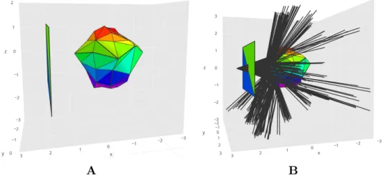
In our first experiment, we consider the situation with the monopole source sitting at
(2.5,0,0). The microphone is atx≈2 and is approximately bounded byy∈[−2,2],
z ∈ [−1.15,1.15]. See figure 3. We run the algorithm with K = 3, β = 0.7 and
µ = 0.18. At this point, we conduct (1, K) search by having the routine choose
dvi0 randomly, as described in section 4.2. For the computation of the partial loss values associated with the triangles, we sample 50 rays casted toward each triangle.
It must be noted that often either all or none of the rays end up intersecting the
microphone plane; however sampling more rays reduces potential variance in the partial loss calculations, making the algorithm more robust.
The resulting shape as determined by the algorithm is shown in figure 4. As one can see, the algorithm is successful in achieving its goal of minimizing the sound
pressure, expressed in the amount of sound rays, at the microphone. It has found
a way to adjust the front triangles such that each ray will either scatter in the
A B
negative xdirection or, if scattered backwards in the positive xdirection, travels
around the microphone plane. This is clearly a consequence of the sharp tip the shape has obtained, which was absent in the case of the sphere.
It is worth noting that the rear of the sphere, at the far away end from the
microphone, was deformed into a seemingly random structure. This is caused by the fact that no rays would hit this side in the first place; as such the quantum algorithm
has no information about it (meaning the quadratic QUBO entries corresponding
to those triangles are zero) and will choose a random vertex in each iteration. As such, it would make sense, in a further version of this algorithm, to prune these
}
Flattened ExtrudingA B
C D
triangles in order to allow processing of more detailed shapes (containing more
elements) on the QPU. In this work, however, we chose not to do this as our wish was to investigate the effect of the algorithm on the entire shape. After all, our
problem was inspired by external vehicle mirror design, which does not allow for
cut shapes. The values forβ andµwere chosen by trial-and-error search, by testing a small set of combinations covering β∈[0.3,1.0] andµ∈[0.15,0.20]. We noticed
that a too low step size renders the algorithm incapable of sufficiently adapting
the shape within the given number of iterations, as it usually gets stuck in a local, suboptimal point, which cannot be optimized any further. This seems to occur in
particular with (1 + [K−1]) search. On the other hand, a too high step size usually
(especially in the case of (1, K) search) produces a too irregular shape. A good example showing the consequence of choosing a too low step size can be seen in
figure 5. Here, we moved the monopole to (0,3,2) and chose a step size control
β = 0.3. We observe that although two sources of loss have been eliminated, one seems to be persistent. The result in figure 5(d) with only two triangles having
nonzero partial loss (which, even though not shown in the figure, is lower than
that of the sphere in fig. 5(c)) is most likely considered as a local optimum by the algorithm, meaning it chooses not to depart from there.
6
Conclusions
In this work, we have presented a finite-element method for optimizing a
three-dimensional shape under given physical criteria. By formulating an approximation
of this finite-element problem in a QUBO form, and by embedding the corresponding matrix on the QPU as specified, we have been able to show that it is possible to
successfully carry out finite-element design optimization on a D-Wave QPU. We
have shown that by supplying an initial shape we can optimize the geometry to minimize a specified quantity, such as sound pressure, at a target area around the
shape or the vibration of single elements, and in the same instance partially preserve
the geometry. This is important, as if we supply the design of an outside mirror of a vehicle and intend to minimize the noise at the passenger’s positions, we still
want to end up with a design that captures all the properties a mirror must have.
Furthermore, we have demonstrated how to usefully combine the computing power of a classical computer with that of a quantum computer. That is, we
calculate the sound pressure on an initial geometry classically and have the QPU
7
Future work
For the next version of the algorithm, we intend to find a formulation that will
incorporate additional constraints on the final shape. In addition, we would like to add wave behaviour corrections to increase the degree of realism in the model,
or alternatively, discard the ray-casting approximation and find a way to model
sound waves directly. Additionally, we wish to explore scalability of the algorithm, as we should be able to process shapes with more elements by splitting the QUBO
matrix with theqbsolvdecomposing solver tool [27], instead of having the D-Wave
software find minor embeddings for shapes with few elements. This will be of use in the future, when we expect new D-Wave QPU generations. With these new chips
having more couplers between the qubits, we will be able to embed shapes with
more elements and hopefully determine smoother geometries. We will continue to focus on laying the foundation for solving practically relevant problems by means of
quantum computing, quantum simulation, and quantum optimization [16, 17, 28–33].
Acknowledgments
Thanks go to VW Group CIO Martin Hofmann and VW Group Region Americas
CIO Abdallah Shanti, who enable our research.
References
[1] Marcello Benedetti, John Realpe-G´omez, Rupak Biswas, and Alejandro Perdomo-Ortiz. Estimation of effective temperatures in quantum annealers for
sampling applications: A case study with possible applications in deep learning.
Physical Review A, 94(2), 2016.
[2] Vadim N. Smelyanskiy, Davide Venturelli, Alejandro Perdomo-Ortiz, Sergey Knysh, and Mark I. Dykman. Quantum Annealing via Environment-Mediated
Quantum Diffusion. Physical Review Letters, 118(6), 2017.
[3] Davide Venturelli, Dominic J. J. Marchand, and Galo Rojo. Quantum Annealing
Implementation of Job-Shop Scheduling. jun 2015.
[4] Zhang Jiang and Eleanor G. Rieffel. Non-commuting two-local Hamiltonians
for quantum error suppression. Quantum Information Processing, 16(4), 2017.
tunneling through quantum Monte Carlo simulations. Physical Review Letters,
117(18), 2016.
[6] B. O’Gorman, R. Babbush, A. Perdomo-Ortiz, A. Aspuru-Guzik, and
V. Smelyanskiy. Bayesian network structure learning using quantum annealing.
The European Physical Journal Special Topics, 224(1):163–188, 2015.
[7] Eleanor G. Rieffel, Davide Venturelli, Bryan O’Gorman, Minh B. Do, Elicia M. Prystay, and Vadim N. Smelyanskiy. A case study in programming a
quan-tum annealer for hard operational planning problems. Quantum Information
Processing, 14(1), 2014.
[8] Davide Venturelli, Salvatore Mandr`a, Sergey Knysh, Bryan O’Gorman, Rupak
Biswas, and Vadim Smelyanskiy. Quantum optimization of fully connected spin glasses. Physical Review X, 5(3), 2015.
[9] A. Perdomo-Ortiz, J. Fluegemann, S. Narasimhan, R. Biswas, and V.N. Smelyanskiy. A quantum annealing approach for fault detection and
diagno-sis of graph-based systems. The European Physical Journal Special Topics,
224(1):131–148, 2015.
[10] Sergio Boixo, Troels F. Rønnow, Sergei V. Isakov, Zhihui Wang, David Wecker,
Daniel A. Lidar, John M. Martinis, and Matthias Troyer. Evidence for quantum annealing with more than one hundred qubits. Nature Physics, 10(3):218–224,
2014.
[11] Ryan Babbush, Alejandro Perdomo-Ortiz, Bryan O’Gorman, William Macready,
and Alan Aspuru-Guzik. Construction of Energy Functions for Lattice
Het-eropolymer Models: Efficient Encodings for Constraint Satisfaction Program-ming and Quantum Annealing. InAdvances in Chemical Physics, volume 155,
pages 201–244. 2014.
[12] J.A. Smolin and G. Smith. Classical signature of quantum annealing. Frontiers
in physics, 2(52), 2014.
[13] Alejandro Perdomo-Ortiz, Neil Dickson, Marshall Drew-Brook, Geordie Rose,
and Alan Aspuru-Guzik. Finding low-energy conformations of lattice protein models by quantum annealing. Scientific Reports, 2, 2012.
[14] Los Alamos national laboratory. D-Wave 2X quantum computer, 2016.
[15] Florian Neukart, Gabriele Compostella, Christian Seidel, David von Dollen,
[16] Florian Neukart, David Von Dollen, and Christian Seidel. Quantum-assisted
cluster analysis. mar 2018.
[17] F. Neukart, C. Seidel, G. Compostella, and D. Von Dollen. Quantum-enhanced
reinforcement learning for finite-episode games with discrete state spaces.
Frontiers in physics, 5(71), 2017.
[18] A. Lucas. Ising formulations of many NP problems. Frontiers in physics, 2(5), 2014.
[19] D.W. Pepper and J.C. Heinrich. The finite element method: basic concepts and applications with MATLAB, MAPLE and COMSOL. CRC press, 3 edition,
2017.
[20] A. Sanz-Garc´ıa, A.V. Pern´ıa-Espinoza, R. Fern´andez-Mart´ınez, and F.J.
Mart´ınez-de Pis´on-Ascac´ıbar. Combining genetic algorithms and the finite
element method to improve steel industrial processes. Journal of Applied Logic, 10(4):298–308, 2012.
[21] T B¨ack, D B Fogel, and Z Michalewicz. Handbook of Evolutionary Computation.
Evolutionary Computation, 2:1–11, 1997.
[22] Thomas B¨ack, Peter Krause, and Christophe Foussette. Automatic
Metamod-elling of CAE Simulation Models. ATZ worldwide, 117(5):36–41, 2015.
[23] Fabian Duddeck. Multidisciplinary optimization of car bodies. Structural and
Multidisciplinary Optimization, 35(4):375–389, 2008.
[24] Arthur Appel. Some techniques for shading machine renderings of solids. In
Proceedings of the April 30–May 2, 1968, spring joint computer conference on
- AFIPS ’68 (Spring), page 37, 1968.
[25] Turner Whitted. An improved illumination model for shaded display.
Commu-nications of the ACM, 23(6):343–349, 1980.
[26] David P. Dobkin, C. Bradford Barber, and Hannu Huhdanpaa. The quickhull
algorithm for convex hulls. ACM Transactions on Mathematical Software, 1996.
[27] D-Wave systems. Qbsolv, a decomposing solver, 2018.
[28] Florian Neukart and Sorin-Aurel Moraru. On Quantum Computers and
Artifi-cial Neural Networks. Signal Processing Research, 2(1), 2013.
[29] Florian Neukart and Sorin Aurel Morar. Operations on quantum physical
[30] Sven Eisenkr¨amer. Volkswagen trials quantum computers, 2017.
[31] Florian Neukart. Quantum physics and the biological brain. In Reverse
Engineering the Mind, pages 221–229. 2017.
[32] Anna Levit, Daniel Crawford, Navid Ghadermarzy, Jaspreet S. Oberoi, Ehsan
Zahedinejad, and Pooya Ronagh. Free energy-based reinforcement learning using a quantum processor. may 2017.
[33] Daniel Crawford, Anna Levit, Navid Ghadermarzy, Jaspreet S. Oberoi, and
Pooya Ronagh. Reinforcement learning using quantum boltzmann machines.
arXiv preprint arXiv:1612.05695v2, pages 1–17, 2016.
[34] T. B¨ack and S. Khuri. An evolutionary heuristic for the maximum independent set problem. In Proceedings of the First IEEE Conference on Evolutionary
Computation. IEEE World Congress on Computational Intelligence, pages
531–535. IEEE.
[35] D-Wave systems. Quantum computing: how D-Wave systems work, 2017.
[36] D. Korenkevych, Y. Xue, Z. Bian, F. Chudak, W. G. Macready, J. Rolfe, and
E. Andriyash. Benchmarking quantum hardware for training of fully visible Boltzmann machines.
[37] Dmytro Korenkevych, Yanbo Xue, Zhengbing Bian, Fabian Chudak, William G.
Macready, Jason Rolfe, and Evgeny Andriyash. Benchmarking Quantum
Hardware for Training of Fully Visible Boltzmann Machines. Frontiers in physics, 2(5), nov 2016.
[38] T. Lanting, A. J. Przybysz, A. Yu Smirnov, F. M. Spedalieri, M. H. Amin,
A. J. Berkley, R. Harris, F. Altomare, S. Boixo, P. Bunyk, N. Dickson, C.
En-derud, J. P. Hilton, E. Hoskinson, M. W. Johnson, E. Ladizinsky, N. Ladizin-sky, R. Neufeld, T. Oh, I. Perminov, C. Rich, M. C. Thom, E. Tolkacheva,
S. Uchaikin, A. B. Wilson, and G. Rose. Entanglement in a quantum annealing
processor. Physical Review X, 4(2), 2014.
[39] Martijn Van Otterlo and Marco Wiering. Reinforcement learning and Markov decision processes. Reinforcement Learning, pages 3–42, 2012.