http://www.jscdss.com Vol.6 No.4 August 2019: 1-9 Article history:
Accepted 8 May 2019 Published online 8 May 2019
Journal of Soft Computing and Decision
Support Systems
A Method for Deploying Relay Nodes in Homogeneous Wireless Sensor
Networks Using Particle Optimization Algorithm
Behnaz Mahdian a, Mohsen Mahrami a,*, Mohsen Mohseni a a
Department of Computer Engineering, Malard Branch, Islamic Azad University, Malard, Iran
* Corresponding author email address: [email protected] Abstract
There are many methods for deploying relay nodes in wireless sensor networks with the aim of increasing network lifetime and reducing energy consumption. To overcome the issue, in this research, we first set the set of probe points for the establishment of relay node s, since our goal is to minimize the number of relay nodes and increase the coupling between relays and sensors. This problem is NP-hard, so in order to solve this problem in a short time, the particle optimization algorithm using a weighted multifunctional function as a meta-burgh solution was used. We used this algorithm for determining the number and location of the placement relay nodes to reduce the number of nodes and increase network lifetime and network performance. We evaluated this proposed method for both theoretical analysis and numerical results. The results showed that the proposed approach provide better results compared to the greedy algorithms and particle optimizations.
Keywords: Wireless Sensor networks, Relay node, Particle optimization algorithm.
1. Introduction
A wireless sensor network is a network that includes a large number of low-cost sensor nodes with limited energy, which it is responsible for receiving information from the environment, analyzing and processing them, as well as sending sensory data to other nodes. Communication between sensors is usually wireless. Each sensor works independently and without human intervention. The sensor is physically very small and there are limitations in processing power, memory capacity and power supply which these limitations create some problem. Although the use of wireless sensor networks is increasing, the design of these networks is a major challenge. To enhance the network performance, various parameters for improvement are considered including area coverage, life span and reliability (Kuila et al., 2013) which can be significantly improved with the exact deployment of the node. The problem of deploying nodes in a wireless sensor network has been solved with different methods and algorithms, in order to improve performance. In a wireless sensor network, taking into account the limitation in energy of the batteries of sensors, it is possibile for a large number of nodes to be damaged during propagation. As well as network nodes have energy constraints and cannot be recharged, therefore, optimal protocols are needed to reduce energy consumption and increase lifespan. One of the methods used in this field is the deployment of the additive relay node. This problem is solved by some
optimization methods. Evolutionary algorithms are also used, in order to select optimal location for add-on sensors, which these methods increase the network lifetime (Liu et al., 2016).
2. The proposed method
We propose a method using particle optimization algorithm. There is a systematic property in particle collective intelligence particle optimization algorithm, that the agents co-operates locally in this system and the collective behavior of all agents leads to the convergence at a point close to the optimal overall solution. The strength of this algorithm is that it does not need an overal control. Each particle (agent) in this algorithm has a relative autonomy that can move across the solution space and have to cooperate with other swarms (agents). A well-known algorithm for collective intelligence is Particle Swarm Optimization (PSO).
PSO is a group of optimization algorithms that operate on the basis of random population generation. This algorithm is based on the modeling and simulation of the flying of a bunch of birds (in group) or movement a bunch of fishes (in group). A group of particle optimization in space is randomly looking for food. There is only one piece of food in the space under discussion. None of the particle optimization knows the food location. To track particles, the smallest distance to the food is the best strategy. This strategy is in fact the source of the algorithm. Each solution
which is called a particle is equivalent to a particle in the particle motion algorithm.
2.1 WSN relay nodes in particle optimization algorithm
In order to obtain a satisfactory performance in the hierarchy of wireless sensor networks, we need to make relay nodes efficient and effective. The focus of the research is to design an algorithm for providing a solution for placing relay nodes in hierarchical wireless sensor networks. In this research, a relay node algorithm is generated for all possible positions for relay nodes. Simulated particle optimization algorithms are designed to optimize positions. The goal is to find an acceptable solution. Each node relay here is equivalent to a particle in the particle optimization algorithm (Degener et al., 2011).
2.2 Objectives of deploying WSN relay nodes in particle optimization algorithm
Three important goals are considered to maximize the lifetime and improve the performance of the given WSN which are: (1) The number of relay nodes is minimize, (2) Energy consumption is minimized and (3) The connection degree between the relay nodes and the sensor nodes is maximize. We study this proposed method with both theoretical analysis and numerical results.
2.3 Determining the initial population of the WSN relay nodes in the particle optimization algorithm
If we consider the number of relay nodes ( ) and the communication range of the sensor nodes ( ) and a flag bit
( ) with an initial value of 0 for each sensor node and possible places for the relays ( ), then we consider the place ( ) as the center of the circle and the radius of the circle ( ) and we check each node, to have a close distance to the relay and covered by relay.
For each node ( ), we calculate the distance with the node ( ) and if the distance between them is
( )that means this node can be considered as the relay node ( ) and a circle is considered with center ( ) and diameter ( ) and each node which is located in this distance its flag bit becomes one (Lloyd et al., 2015).
For each node ( ), we calculate the distance with the
node ( ) and if the distance between them is
( ) that we can consider the node ( ) as ( ), we consider a circle for this circle node which its center ( )
and its radius is ( ) and each node which is covered, will be flippe to one.
For each node ( ), we calculate the distance with the node ( )and if the distance between them is ( ), for each of these two nodes we consider different circles with their centers are ( ) and ( ) and their radius ( ) and each of the nodes which is covered will be flipped to one. This is done for all nodes, and a number of relay nodes are eventually nominated and introduced.
Primary relay nodes are a set of relay nodes, or the provided solutions for placing relay nodes and their
positioning . Each relay node indicates situations that may be the optimal solution for deploying relay nodes for optimal network performance.
In this algorithm, in addition to the initial random location of particles, a value is also allocated for the initial particle velocity. The initial suggested range for velocity of particles can be extracted from the following equation.
(1)
where ( ) represents the speed of each relay node, and
( ) represents the position of the relay nodes in the WSN network.
Increasing the number of primary relay nodes reduces the number of repetitions needed to converge the algorithm. Although increasing the number of primary relay nodes reduces the number of repetition, this increase causes the algorithm to spend more time in the evaluation of the relay nodes, and subsequently, the execution time until the convergence of the algorithm does not decrease, despite a decrease in the number of repetit . So increasing the number of relay nodes cannot be used to reduce the runtime of the algorithm. In order to reach the optimal solution, the number of repetitions in algorithm increases (if the convergence condition is such that the cost of the best relay node does not change in several successive repetitions), which ultimately the runtime to reach the optimal solution is not decreased. It should also be noted that the reduction of the number of relay nodes may cause the restriction to the local minima, and the algorithm does not reach to the main minimum solution. If we consider a number of repetitions as the convergence condition, although it reduces the number of initial particles, the run time of algorithm will be reduced, but the obtained solution will not be an optimal solution of the problem. Because the algorithm is executed incompletely. Therefore, in this algorithm, reaching to the optimal solution will be as the ending condition of the algorithm (Lu et al., 2010).
2.4 Calculation of fitness function
In this step, we need to evaluate each relay node in the WSN, which represents a solution to the problem. Each relay node in the WSN has a complete information about the input parameters of the problem, which this information is extracted and considered in the objective function.
One of the fundamental steps that we should address is the definition of a fitness function for evaluating the quality of the relay nodes in the WSN of the initial population, as well as evaluating their quality in the next steps. Since a criterion for the particles or better generation must be determined in the particle optimization algorithm, so that these types of particles are preserved for continuation and remaining be removed, so it is crucial to determine this evaluation function (Lee et al., 2010).
The three goals in this article are studied. Minimizing the number of relay nodes, minimizing energy consumption, maximizing communication between relay nodes and sensor nodes in wireless sensor networks. Firstly, we convert them to mathematical equations, and then we obtain the sum of weights for constructing a multi-objective fitness function. To reduce the complexity of the fitness function, we obtain the number of relay nodes in the fitness function. We use the weight ( ) and ( )where we have (( ))and consider the weights as
and compute the optimal solution. For each node of the sensor, we choose a solution to select the best particle that means assigning relay nodes. The objectives are:
i. Use a connection to measure the redundancy of the relay nodes.
ii. For each sensor node, if there are no available relay nodes, use the number of available sensor paths.
iii. The nodes directly indicate the connection, otherwise the excess load ratio will be reduced in order to prevent excessive distribution of congestion (Rawat et al., 2014).
( ) (2)
where is the number of available paths and factor is constatnt considered to be 0.15.
For the number of nodes, we use the following formula, which is equal to ( ( ) ). is the number of relay nodes (Karl et al., 2016). is the threshold distance between free space and the fade of several paths. If the distance between a sensor node and its relay node is greater than the threshold, then the multiple path will be used. is the distance between a sensor node and a relay node in a multiple path. For k bit energy consumption, we have (Min et al., 2015):
( ) ( ) ( ) ( )
(3)
where is energy consumption, dthuris the threshold distance between free space and the fade of several paths,
is the distance between a sensor node and a relay node in a multiple path, is the numbr of bit energy
consumption, and is is the energy
required by the free space.
If we want to express the fitness function in the language of probabilities, we can say that or the weight of each index expresses its probabilistic value. So we have:
( ) ( ) ( ) (4)
where ( ) is a known nonlinear, ( ) is energy consumption and is the weight of each index.
Such that and our goal is to minimize the value of the fitness function. In other words:
* + (5) Therefore, each node of the WSN relay whose value of the fitness function has the lowest value is considered the best solution. Record the best position for each WSN relay node ( ) and the best position among all WSN ( ) relay nodes. At this stage, according to the number of repetitions, two states can be checked.
i. If we are in the first repetition ( ). The current position of each WSN relay node is the best location found for that WSN relay node.
( )
( ) ( ( )) (6)
where is the best position for each WSN relay node and is the best position among all WSN relay nodes, cost is the cost function for PSO algorithm, ( ) is the position of particle .
ii. In other repetitions, we compare the cost of WSN relay node in Step 2 with the best cost for each WSN relay node. If this cost is less than the best-recorded cost for this WSN relay node, then the location and cost of this WSN relay node will replace the previous value. Otherwise, location and recorded cost for this WSN relay is calculated as:
{ ( ( )) ( )
⇒ {
( ) ( ( ))
( )
(7)
2.5 Updating the speed and position of the WSN relay nodes
The speed vector update for all WSN relay nodes is performed as follows:
i( ) i( ) 1 1 ( i( ) 2 2
( i( ) (8)
where ( ) is current velocity, ( ) is updated velosity, is inertia weight, and are acceleration (learning) factors, 1 and 2 are uniformly distributed random numbers between 0 and 1, ( ) is current position of particle i.
these coefficients positive and in range from 1.5 to 1.7 (Romer et al., 2017; Tilak et al., 2014).
In other words, these WSN relay nodes move in the n-dimensional space of the problem in a repeating manner, to search for possible new solution by calculating the appropriate values as a evaluation criterion.
The velocity vectors and position of each of the WSN relay nodes in each repetition of the algorithm are calculated as follows (Younis et al., 2017).
( ) ( ) (9)
(10)
(11)
{
(12)
In the above relation, the new speed vector of each WSN relay node is computed based on its previous speed of the WSN relay nodes , the best position that the WSN
relay nodes have achieved so far ( ) and the location of the best WSN relay node in the neighborhood of WSN relay node ( ). If the neighbors of each WSN relay node include all of the WSN relay nodes of the group, then
represents the position of the best WSN relay node in the group that is referred to ( ). ( )are two random numbers (with a uniform distribution between [0,1]) that are produced independently of each other. In this equation, is a definition used in Eq. (12).
and which are learning coefficients are considered positive in a range from 1.5 to 1.7, which controls the effect of ( and ( on the search process. denotes the inertial weighting coefficient. We measure this coefficient positive and in range from 0.7 to 0.8.
The speed vector of the WSN relay node is limited to . is a limitation that controls the global search capabilities of the WSN relay node. By using Eq. (12), the speed vector of each WSN relay node is converted to the probability vector of the variation. In the above relation,
represents the probability that is equal to 1. Then,
using Eq. (12), the location vector of each WSN relay node is updated. In the above relation, is a random number with a uniform distribution between zero and one. The problem space is equal to the number of parameters in the desired function for optimization. A memory is assigned to store the best position of each WSN relay node in the past, and a memory to store the best available position among all the WSN relay nodes. The WSN relay node decides how to move in the next step, achieving the experience of these memories. At each repetition, all the WSN relay nodes move in the n-dimensional space of the problem so that a general optimal point can finally be found. The WSN relay nodes update their speeds and their location according to the best local and absolute solutions. The result is the following formula (Gupta et al., 2017).
new( ) old( ) new( ) (13)
where ( ) is the speed of the WSN relay nodes, is the WSN relay nodes variables, is random numbers with
uniform distribution, are learning factors, is the local best ( ), is the global best and , the best absolute answer.
The particle algorithm updates the velocity vector of each WSN relay node and then adds the new speed value to the position or value of the WSN relay. Updating the speed are affected by both values, the best local solution and the best absolute solution.
The best local solution and the best absolute solution are the best solutions achieved till the current running time of the algorithm, by a WSN relay node and in the whole population, respectively. The constants are called Perceptual Parameter and Social Parameter respectively, respectively. The main advantage of the WSN relay node is that the implementation of this algorithm is simple and needs a few parameters. Particles are also able to optimize complex cost functions with a large number of local minima (Ataul et al., 2010; Maheshwari et al., 2016).
2.6 Convergence Test
The convergence test in this algorithm is similar to other optimization algorithm. There are various methods for checking the algorithm. The method most often used in the convergence test of the algorithm is that if there is no changes in cost of the best node of the WSN relay, after several consecutive repetitions, and then the algorithm ends, otherwise it should return to the previous step (Younis et al., 2004).
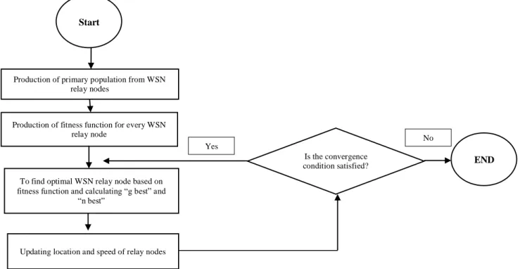
2.7 Diagram of suggested algorithms
The flowchat of the proposed algorithm is shown in Fig.
1.
3. Analysis and calculated results
In this section, we will analyze the results of simulation of the algorithm for deploying proposed relay nodes. The simulation was performed using the 2016 software.
3.1 How to simulate the proposed algorithm
earned in the previous repetition and so an algorithm runs until satisfying the convergence condition.
3.2 Evaluation criteria
The purpose of this paper is to determine the minimum number of relay nodes as well as their optimal position to enhance the performance of wireless sensor networks with maintaining the ability of connecting all sensor nodes and
balances between relay nodes for proper distribution and uniform use of energy.
Therefore, in order to evaluate the efficiency and performance of the proposed algorithm, the ratio of the number of selected prone positions, compared with the number of sensor nodes, the number of different default positions, the number of connectivity capabilities for each sensor node (the number of relay nodes located in coverage zone of a sensor node antenna) and coverage domain of sensor nodes antenna.
Fig. 1. Structure of optimization algorithm of proposed group.
3.3 Simulation Parameters
Matlab software was used to evaluate the proposed algorithm. The computer with Intel Ci5 processor and 4 GB memory and Windows 7 operating system was used. A scenario of wireless networks in an area of 200 to 200 square meters was used for simulation and 200 nodes of the wireless sensor were randomly distributed. The central station was located in the middle of the enclosure, with coordinates 100 and 100 . The primary energy for each node is 0.5. The communication range for each sensor node was 50 meters . In this simulation, the initial population of the possible solution for the proposed algorithm was equal to 100 particles and randomly generated. Each particle is, in fact, an arrangement or deployment of relay nodes in primary prone locations where both their number and their location are randomly selected. The default number of repetitions was 200, but, the algorithm ends before the runs out time, if there are no more optimal changes. The condition is determined by counting the total number of designated locations for deployment of relay nodes, that means, when it is recognized that the mentioned value is not decreasing and no better optimal state occurs, then the
algorithm ends. The minimum number of relay nodes for each sensor node with communication power ( ) choosed 2. The setting for simulation is given in Table 1.
3.4 Simulation results
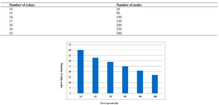
In Fig. 2, the variation in the number of relays by the number of sensor nodes is represented . In this evaluation, we repeat the algorithm with 300 location. In Table 2, we show the simulation results. In this scenario, the stability of the algorithm with respect to changes in the number of sensor nodes and the number of relay location is evident.
The results shows the output of algorithm (number of relay nodes) with respect to the number of sensor nodes, indicating that in general, with the increase in the number of wireless sensor nodes, the number of relay nodes also increases to some extent, but it can be said The number of relay nodes does not depend to the number of sensor nodes directly but, depends on dispersion of nodes directly. The results indicate that the low number of sensor nodes does not lead to the reduction of the number of selected relay nodes. Fig. 3 presents the dispersion of the relay nodes by increasing the coverage domain of the wireless sensor nodes. In this evaluation, the number of sensor nodes equal to 300 nodes, the number of relay nodes equal to 100
No Production of primary population from WSN
relay nodes
Start
Production of fitness function for every WSN relay node
To find optimal WSN relay node based on fitness function and calculating “g best” and
“n best”
Updating location and speed of relay nodes
Is the convergence condition satisfied? Yes
primary relay nodes, the initial population of particle optimization algorithm equal to 100 particle and connectivity degree equal to 2. Other parameters were implemented according to the information of simulation base table. Fig. 3 shows the variation of the number of optimally selected relay nodes by the proposed algorithm
with respect to the antenna coverage domain of the sensor nodes . The results show that with increasing coverage domain in wireless sensor nodes, the number of relays decreases. In this diagram, the horizontal axis represents the coverage range and the vertical axis represents the number of relay nodes.
Table 1
Simulation Parameters.
Parameter Amount
Simulation area (level) 200 * 200 square meter
Location of the central station (100,100)
Sensor nodes 200
Initial population of particle optimization algorithm 100
Number of iteration of simulation 200
Communication scope 50 m
Primary energy nodes 0.5
Fig. 2. variation of number of relays number with the number of sensor nodes.
Table 2
Relay number variation with the number of sensor nodes.
Number of nodes Number of relays
20 10
50 15
100 18
150 17
200 20
250 18
300 19
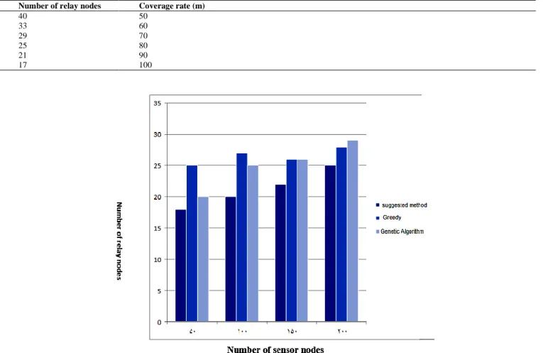
Table 3 shows the variation of the optimally selected number of relay nodes by the proposed algorithm with respect to the coverage zone of sensor node antenna. Numerical analysis shows that with increasing coverage domain in wireless sensor nodes, the number of relays decreases. The proposed algorithm compared with two methods of greedy and the traditional particle optimization method is carried out. In this evaluation, the number of relay nodes used in the network is investigated by increasing the number of sensor nodes. Fig. 4 shows that the proposed method provides better results than greedy algorithms and particle optimizations. At the same amount of considered limited WSN space, the proposed algorithm can be used to reduce the number of relay nodes comparing
to greedy and genetic algorithms. The proposed algorithm requires less number of relay nodes than the other two algorithms for use in the same number of sensor nodes. The number of relay nodes increases with increasing number of sensor nodes, but when the number of sensor nodes reaches a certain number, the number of relay number decreases. The reason is that because the network is dense, there is no need to add additional relay nodes. As a result, the results are better than the other two algorithms. Fig. 4 shows the ratio of the number of relay nodes with respect to the number of sensor nodes. In Fig. 4, the horizontal axis represents the number of sensor nodes and the vertical graph representing the number of relay nodes.
Table 3
Changes in the number of optimally selected relay nodes by the proposed algorithm.
Coverage rate (m) Number of relay nodes
50 40
60 33
70 29
80 25
90 21
100 17
Fig. 4. Comparison of proposed algorithms with previous algorithms
Also, you can numerically compare the proposed method with other methods. In this evaluation, the number of relay nodes used in the network is investigated with increasing the number of sensor nodes. And these numerical parameters are given in the following table. As the results show, the proposed algorithm requires less
Table 4
Comparison of proposed algorithm with previous algorithms
Number of sensor nodes Recommended method of relay number
Greedy Number of relays Particle optimization algorithm Relay number
50 18 25 20 100 20 27 25 150 22 26 26 200 25 28 29
4. Discussion
In this research, a new algorithm for relay node assignment for wireless sensor networks was presented under the name of relay node deployment based on particle optimization algorithm. In fact, this algorithm is an appropriate locating method and a reduction in the number of relay nodes, which by using the power of the particle optimization algorithm attempts to reduce the overall cost of creating a network by reducing the number of relay nodes, as well as increasing the network lifetime. The focus of the research is to design an algorithm for providing a solution for placing relay nodes in hierarchical wireless sensor networks. In this research, a relay node algorithm is generated for all possible positions for relay nodes. Simulated particle optimization algorithms are designed to optimize positions. The goal is to find an acceptable solution. Three important goals are considered to maximize the lifetime and improve the performance of the WSN given. The goals are to minimize the number of relay nodes and minimize energy consumption, and maximize the connection degree between relay nodes and sensor nodes. The most important innovation in this research was the use of the metha-heuristic method of particle optimization algorithm in determining the of minimum possible numbers for the deployment of relay nodes as well as determining the optimal location of their placement, which has a significant effect on reducing the network cost and good connectivity. Another innovation of this research is in the type of using the particle optimization algorithm, which includes coding of the particles of the problem (relay node location solutions), the selection step, the definition of the fitness function, taking into account the stated objectives that are reflecting the number of selected optimal locations, as well as the connectivity function that was designed to rank the initial positions for k-connectivity. Another phase of the particle optimization algorithm which has an innovation is the step used to reduce the number of relay node deployment by removing the locations that have the lowest score (the highest value of the fitness function).
5. Conclusion
The simulation results of the proposed algorithm were presented to determine the optimum number and position of the relay node deployment based on the particle optimization algorithm. The capabilities of the proposed algorithm were shown in reducing the number of primary feasible conditions and thus reducing the cost of creating the network. According to the diagrams and simulation results, it was proved that the proposed algorithm is stable
with respect to the changes more than a certain number of Sensor nodes and relay nodes and provide the minimum number of relay nodes for network coverage with proper connectivity. The results showed that the efficiency of the proposed algorithm has a good ability in determining the optimal relay locations and their minimum number. Applying other useful parameters to determine fitness function, the use of the proposed method for clustering sensor nodes in communicating with relay node and the use of other methods and hybrid methods to determine the optimal number and position of the location of relay nodes (eg by neural networks) are the main suggestions for the future studies.
References
Ataul, B. (2010). Clustering strategies for improving the lifetime of two-tiered sensor networks Computer Communications. 31 (1), 3451–3459.
Birla, D., Maheshwari , P., & Gupta, H.O. (2016). A new nonlinear directional overcurrent relay coordination technique, and banes and boons of near-end faults based approach. IEEE Transactions on Power Delivery, 21(3), 1176–1182.
Degener, B., Fekete, S. P., Kempkes, B., & Auf Der Heide, F. M. (2011). A survey on relay placement with runtime and approximation guarantees: Computer Science Review, vol.5 (1), pp. 57-68.
Gupta, G., Younis, M. (2007). Load-balanced clustering of wireless sensor networks, in: Proceedings of IEEE International Conference, ICC '03, vol. 3 pp. 1848–1852. Romer, K., & Mattern, F. (2017).The Design Space of Wireless
Sensor Networks. IEEE Wireless Communications, Vol. 11, No. 6, Dec.
Karl, H., and Willig, A. (2016). Protocols and Architectures for Wireless sensor Networks, Wiley, United Kingdom, April. vol.56 (1), pp.1-44.
Kuila, P., Gupta, K., & Jana, K . (2013) . A novel evolutionary approach for load balanced clustering problem for wireless sensor networks : Swarm and Evolutionary Computation, 56-48,12.
Lee, S. (2010). Optimized relay node placement for federating wireless sensor sub-networks: University of Maryland at Baltimore County.
Liu, H., Wan, P., & Jia, X. (2016). On optimal placement of relay nodes for reliable connectivity in wireless sensor networks: Journal of Combinatorial Optimization, vol. 11(2), pp.249-260.
Lloyd, E. L., & Xue, G. (2015). Relay node placement in wireless sensor networks: Computers, IEEE Transactions on, vol.56 (1), pp.134-138.
Lu, K., Chen, G., Feng, Y., Liu, G., & Mao, R. (2010). Approximation algorithm for minimizing relay node placement in wireless sensor networks: Science China Information Sciences, vol.53 (11), pp.2332-2342.
Algorithm for Restoring Inter-node Connectivity in Networks of Moveable Sensors," IEEE Transactions on Computers (to appear).
Min, R. (2001). Low Power Wireless Sensor Networks, Proc. of the International Conference on VLSI Design, Bangalore, India, January, 54-44,12.
Younis, O., Fahmy, S. (2004). a Hybrid, Energy-Efficient, Distributed clustering approach for Ad Hoc sensor networks, IEEE Transaction on Mobile Computing 366–379.
Rawat, P., Singh, K. D., Chaouchi, H., & Bonnin, J. M. (2014). Wireless sensor networks: a survey on recent developments and potential synergies. The Journal of supercomputing, vol.68 (1), pp.1-48.
Tilak S. (2014). "A Taxonomy of Wireless Micro-Sensor Network Models," SIGMOBILE Mob. Comput. Commun, Rev., Vol. 6, No. 2. pp. 28-36.