Parisa Mapar
School of Electrical Engineering
Thesis submitted for examination for the degree of Master of Science in Technology.
Espoo 23.5.2018
Thesis supervisor:
Prof. Juho Rousu
Thesis advisors:
Ph.D. Markus Heinonen
school of electrical engineering master’s thesis
Author: Parisa Mapar
Title: Machine Learning for Enzyme Promiscuity
Date: 23.5.2018 Language: English Number of pages: 6+71 Department of Computer Science
Professorship: Computer Science Supervisor: Prof. Juho Rousu
Advisors: Ph.D. Markus Heinonen, Ph.D. Sandor Szedmak
With the discovery of an increasing number of catalytically promiscuous enzymes, which are capable of catalyzing multiple reactions, the traditional view of enzymes as highly specific proteins has been brought into question. The significant implications of protein promiscuity for the theory of enzyme evolution suggest that this inherent feature can be utilized as the seed for engineering new functions in biotechnology and synthetic biology as well as in drug design. Therefore, understanding protein promiscuity is becoming even more important as it provides new insights into the evolutionary process that has led to such vast functional diversity. While there have been numerous efforts devoted to recognizing the determinants of promiscuity, till date, this pertinent question regarding the distinctions between specialized enzymes and promiscuous enzymes has remained unanswered.
As an in silico approach, in this thesis, we attempt to find a predictive model which can accurately classify unseen proteins into catalytically promiscuous and non-promiscuous. To this end, we exploit different representations and properties of proteins, and adopt different computational approaches accordingly. The role of proteins sequences as indicators of promiscuity is investigated by means of the BLAST algorithm as well as string kernels. Additionally, to validate the interplay between proteins’ three-dimensional structures and their promiscuous behaviors, we employ a novel method which is modeling the topological details of proteins as graphs. Graph kernel functions are then applied to measure the structural similarities between the 3D structures of proteins. The classification is performed using SVM as a kernel-based method. The results indicate that proteins’ sequences have limited bearings on promiscuity. Conversely, proteins’ 3D structures can reliably predict whether a protein has promiscuous activities with an accuracy of 96%. Our best results are achieved using the Weisfeiler-Lehman subtree graph kernel and the secondary structure information of proteins.
Keywords: enzyme promiscuity, proteins, machine learning, classification, BLAST, kernel methods, SVM, string kernels, graph kernels
Preface
Foremost, I would like to express my profound gratitude to my supervisor, Prof. Juho Rousu, for offering me the opportunity to conduct this research under his supervision at the Department of Computer Science, for his patience, endless support, and immense knowledge. My sincere thanks also goes to my advisors, Dr. Markus Heinonen and Dr. Sandor Szedmak, for steering me in the right direction with their insightful and valuable comments.
I would also like to thank the current members and alumni of Prof. Rousu’s research group for all their help and friendship, and creating a vibrant environment. My thanks also goes to my friend, Clemens Westrup, for his constructive comments on my thesis and supporting me throughout the process of writing.
Also, I thank all my friends for their unwavering support and in particular, I want to give special thanks to Nanna Koivula for her true friendship and unfailing support. My parents deserve a particular note of thanks as I am forever indebted to them for their unconditional love and continuous encouragement throughout my years of study. Lastly, I would like to express my deepest thanks to my sister, Farimah Mapar, who has been not only my best friend, but also the best guide and inspiration in every step of my life.
Helsinki, 23.5.2018
Contents
Abstract ii
Preface iii
Contents iv
Symbols and abbreviations vi
1 Introduction 1
1.1 Problem Statement . . . 4
1.2 Related Work . . . 4
1.3 Research Scope and Objectives . . . 5
1.4 Protein Structure . . . 6
2 Data 8 2.1 Promiscuity . . . 8
2.2 Data Preprocessing . . . 8
2.3 Datasets . . . 9
2.3.1 The Sequence Dataset . . . 9
2.3.2 The 3D Structure Datasets . . . 11
3 Methods 12 3.1 BLAST . . . 12
3.2 Instance-Based Learning . . . 13
3.3 Kernel Methods . . . 13
3.3.1 Sequence-Based Kernels . . . 16
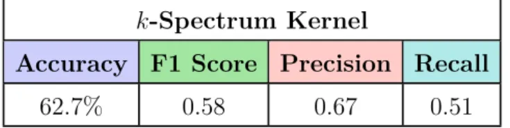
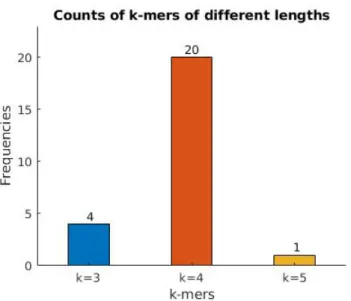
3.3.1.1 The k-Spectrum Kernel . . . 17
3.3.1.2 The Generic String Kernel . . . 17
3.3.1.3 k-NN . . . 18
3.3.2 3D Structure-Based Kernels . . . 19
3.3.2.1 The Graphlet Kernel . . . 22
3.3.2.2 The Weisfeiler-Lehman Subtree Kernel . . . 24
4 Experimental setting 27 4.1 Performance Measures . . . 27 4.2 Balanced Datasets . . . 29 4.3 Cross-Validation. . . 29 4.4 SVM . . . 30 5 Results 31 5.1 Sequence-Based Models. . . 31 5.1.1 BLAST . . . 31
5.1.3 The Generic String Kernel . . . 34
5.1.3.1 k-NN . . . 39
5.2 3D Structure-Based Models . . . 39
5.2.1 The Graphlet Kernel . . . 39
5.2.2 The Weisfeiler-Lehman Subtree Kernel . . . 43
5.3 Data Visualizations . . . 49
5.3.1 k-Spectrum Kernel Visualization . . . 50
5.3.2 Generic String Kernel Visualization . . . 51
5.3.3 Graphlet Kernel Visualization . . . 52
5.3.4 Weisfeiler-Lehman Subtree Kernel Visualization . . . 53
6 Discussion 54 6.1 Sequence-Based Models. . . 54 6.2 3D Structure-Based Models . . . 55 6.3 Future Directions . . . 56 References 57 Appendices 64 A Categorical Features . . . 64
B Vectorial Representations of Features . . . 65
Symbols and abbreviations
Symbols
Å ÅngstromAbbreviations
3D Three-Dimensional AA Amino AcidBLAST Basic Alignment Search Tool BLOSUM BLOck SUbstitution Matrix Cα Alpha-carbon
CCA Canonical Correlation Analysis CV Cross-Validation
DSSP dictionary of protein secondary structures EC number Enzyme Commission number
FN False Negative FP False Positive GP Gaussian Processes GS kernel Generic String kernel
GWSK Gap-Weighted Subsequence Kernel IBL Instance-Based Learning
MDS MultiDimensional Scaling OHE One Hot Encoding
PCA Principal Component Analysis PDB Protein Data Bank
SSE Secondary Structure Elements SVM Support Vector Machine TN True Negative
TP True Positive
WASK Weighted All-Substrings Kernel WL Weisfeiler-Lehman
The genetic information of a cell is carried by its cellular DNA which consists of thousands of genes. Each gene is a segment of the DNA molecule and contains instructions that, when decoded, serve as a recipe on how to build unique, large and complex molecules, called proteins. Therefore, the function of each cell is determined by its decoded genes, which in turn, lead to a collection of formed proteins that perform specialized functions depending on their unique compositions. Proteins are assembled with different amino acids joined together to form long chains, which are then folded into a variety of three-dimensional structures held together by different bonds. The folded shape, or conformation of a protein is dictated directly by its linear sequence of amino acids. As workhorses of the cell, protein macromolecules have an enormous array of indispensable functions within organisms, ranging from providing structure and support for cells, DNA replication, and acting as antibodies to transporting molecules from one location to another. However, the best-known role of proteins in the cell is catalyzing biochemical reactions. These type of proteins, which are called enzymes, act as catalysts by accelerating the chemical reactions inside living cells without being consumed or permanently altered.
In a chemical reaction, one or more chemical substances, known as reagents, reactants, or substrates, are transformed into other types of substances, called products. Enzymes facilitate the occurrence of almost all metabolic processes in the cell, which are impossible under ordinary conditions. These substrate molecules are acted upon and subsequently converted into products by binding to a region on the surface of enzymes, called the active site [Alberts et al., 2002].
The classical definition of enzymes refers to them as remarkably specific catalysts. It suggests that enzymes are usually highly specific as to what substrate they bind to as well as the chemical reaction they catalyze, meaning that they selectivity accommodate certain substrates, referred to as substrate specificity and catalyze specific reactions, known as reaction specificity. These specificities are achieved by binding sites which have complementary shapes and physicochemical characteristics to the substrates. While the notion of “one enzyme—one substrate—one reaction”, which attributes enzyme catalysis to precise optimization of an enzyme for one substrate and reaction, is dominant, there has been a growing appreciation in recent years that this picture is oversimplified [Copley, 2003; Khersonsky and Tawfik, 2010]. Many, if not most, enzymes exhibit capabilities of transforming multiple substrates or catalyzing various reactions, in addition to the ones for which they evolved. An increasing number of enzymes have been reported to enjoy such inherent property referred to as ‘promiscuity’. According to previous reviews, promiscuity can be described based on a wide range of fundamentally different phenomena. Some studies [Patrick et al., 2007; Khersonsky and Tawfik, 2010] define promiscuity as the ability of an enzyme to catalyze secondary adventitious reactions that are not part of the organism’s physiology, which is referred to as ‘catalytic promiscuity’ [O’Brien and Herschlag, 1999]. Hult and Berglund, on the other hand, classify enzymatic promiscuity into three major types that can be combined: substrate promiscuity, which is shown by enzymes with relaxed or broad substrate specificity, catalytic
promiscuity, and condition promiscuity which applies to the enzymes with catalytic activity in a variety of temperatures, pH, etc. [Hult and Berglund, 2007] (see Figure
1). Pyruvate decarboxylase [Hult and Berglund, 2007], carbonic anhydrase [Pocker and Stone, 1967], pepsin [Reid and Fahrney, 1967], chymotrypsin [Nakagawa and Bender, 1969], and L-asparaginase [Jackson and Handschumacher, 1970] are among early examples of catalytically promiscuous enzymes [Khersonsky and Tawfik, 2010]. Promiscuity, however, is distinguished from moonlighting [Jeffery, 1999], which is the utilization of protein parts outside its active site scaffold for additional functions that are mostly regulatory and structural [Copley, 2003].
Figure 1: Mechanistic classification of enzyme promiscuity into three types: (A) Substrate promiscuity or multispecificity; (B) Catalytic promiscuity; (C) Conditional promiscuity [Piedrafita et al., 2015].
During the past two decades, enzyme promiscuity has received considerable attention for its practical applications and has begun to be recognized as a valuable source of information in enzyme evolution [O’Brien and Herschlag, 1999; Copley, 2003]. As early as 1976, Jensen proposed that promiscuity shaped the evolution of protein evolution by suggesting that primitive ancient enzymes which presumably had minimal gene content possessed very broad specificities in contrast to modern enzymes that tend to specialize in one substrate and reaction [Jensen, 1976]. He conceptualized the evolvability of proteins as a process whereby the catalytic versatility enabled a relatively limited arsenal of rudimentary enzymes to afford a wider range of functions that were necessary to maintain ancestral organisms [Khersonsky et al., 2006; Khersonsky and Tawfik, 2010]. Concurrently, in 1977, Jacob postulated in his classical note “Evolution and Tinkering” [Jacob, 1977] that new functions were not produced from scratch, but rather from preexisting suboptimal functions [Khersonsky and Tawfik, 2010]. It is widely accepted that new protein structures and functions were generated from their ancestors whose genes were modified, or ‘tinkered with’
[Khersonsky et al., 2006]. This view, which is supported by many elegant studies, suggests that divergence of enzymes started with ancestral promiscuous enzymes that were changed due to the environmental selection pressure, gene duplication, and mutation resulting in higher metabolic efficiencies [Khersonsky and Tawfik, 2010;Baier et al., 2016]. This process has led to the creation of enzyme families and superfamilies [Gerlt and Babbitt, 2001] whose members share similar scaffold and active site architectures (see Figure 2). For instance, organophosphate hydrolase and atrazine chlorohydrolase are xenobiotic degrading enzymes which evolved from precursor promiscuous enzymes that possessed those functions as their latent activities [Seffernick et al., 2001;Afriat-Jurnou et al., 2012;Baier et al., 2016]. Conservation of structural and catalytic features in theα/β-hydrolase folds in the enolase superfamily is another example suggesting that within each superfamily, enzymes with different substrate and reaction specificities arose from a common ancestor via divergent evolution [Babbitt and Gerlt, 1997; Gerlt and Babbitt, 1998; O’Brien and Herschlag, 1999].
Figure 2: Schematic representation of enzyme evolution within a theoretical enzyme superfamily. Enzymes and their native physiological functions are represented by circles and colors, respectively [Baier et al., 2016].
The importance of promiscuity from an enzymological point of view and its potential mechanistic and evolutionary implications were first highlighted by O’Brien and Herschlag [O’Brien and Herschlag, 1999] and later by Copley [Copley, 2003]. According to them, protein promiscuity is an advantageous feature which can be leveraged to obtain starting points for the evolution of novel enzyme activities. This implies that existing catalysts can be improved by exploiting enzyme promiscuity which ultimately leads to novel metabolic pathways that are currently unavailable
[Hult and Berglund, 2007]. Therefore, relaxed substrate and reaction specificity is a new frontier for biocatalysis and direct evolution. Today, protein promiscuity has fueled much of the growth in biotechnology and synthetic biology by facilitating a better understanding of the evolution of new functions. Indeed, protein engineers have succeeded in tailoring innovative proteins by mimicking this natural process in the laboratory [Kazlauskas, 2005; Peisajovich and Tawfik, 2007; Turner, 2009]. Besides protein engineering, enhanced understanding of promiscuity finds application in drug design for both biomedical or industrial applications [Nobeli et al., 2009]. However, it is worth mentioning that some studies consider promiscuity also as a hurdle jeopardizing the performance of synthetic systems with unwanted side effects [Nobeli et al., 2009].
1.1
Problem Statement
The potential applications of enzyme promiscuity have motivated the search of viable starting places with measurable activities for the development and engineering of novel biocatalysts. However, predicting and rationalizing the existence of promiscuous activities from a given sequence, structure, and native function are challenging tasks with daunting complexity [Babtie et al., 2010]. While some enzyme families have been extensively characterized, our current knowledge of potential factors that influence promiscuity is still limited and biased towards these few examples [Babtie et al., 2010]. For instance, some studies associate promiscuity with conserved regions in the active site [Anandarajah et al., 2000]. Nevertheless, it is not yet resolved to what extent we can generalize these observations to other enzymes. Therefore, in order to uncover determinants that can help us predict the promiscuity, we need to test a large repertoire of enzymes for potential characteristics. Quantitative, mechanistic or structural characterization of promiscuous enzymes can aid in revealing undeveloped or unrealized promiscuous activities in enzymes that currently appear to be highly specific. Furthermore, understanding the mechanistic and structural basis for catalytic promiscuity can provide opportunities for annotating previously uncharacterized enzymes.
1.2
Related Work
In spite of the intense efforts being devoted, till date there is no clear pattern linked to promiscuity which can be generalized to all enzyme families and superfamilies. In this context, various computational tools have attempted to predict and quantify promiscuity. In one study, a quantitative index for assessing the degree of substrate promiscuity based on the catalytic efficiencies has been proposed [Nath and Atkins, 2008]. This index, which computes the degree of variability between different sub-strates, lacks scalability as it targets only a predefined set of substrates. Moreover, assuming the same chemical transformation for all substrates makes this approach applicable only to substrate promiscuity. On a more general level, another study has aimed to predict both catalytic and substrate promiscuity using a sequence-based kernel with protein sequences as the input [Carbonell and Faulon, 2010]. For an
en-zyme with known catalytic activity, this method also tries to investigate promiscuous activities by evaluating similarities between its reactions via graph-based representa-tions of them. While this is an effective method, it does not take into account the protein structures which have proved to carry significant information regarding their biological functions and evolution. Chakraborty and Rao, on the other hand, exploit the 3D structures of proteins to compute their relative promiscuity via an index derived from the spatial and electrostatic properties of the catalytic residues, modeled as signatures [Chakraborty and Rao, 2012]. For a protein with known active site residues and 3D structure, this index ranks its promiscuity based on the number and quality of different active site signatures that have congruent matches in the vicinity of its native catalytic site, as well as differences in enzymatic activities. However, investigation of the role of residues beyond the active site in promiscuity might add new dimensions to our understanding of the interplay between protein structure and its function. Another attempt at leveraging the 3D structures of proteins to predict promiscuity has been discussed in [Steinkellner et al., 2014], where they mine structural databases using active site constellations to identify promiscuous ene-reductase activity. They have shown that typical Old Yellow Enzyme substrates and ligands have equivalent binding modes in their high-resolution crystal structures despite completely different amino acid sequences, overall structures and protein folds. A genome-wide method which aims to predict promiscuous functions of genes in a systematic and unsupervised manner has been proposed as well in a recent study [Oberhardt et al., 2016]. This approach utilizes an unsupervised PSI-BLAST based method to predict promiscuous ‘replacer’ functions that may compensate for primary ‘target’ functions of genes in E. coliif they are altered or lost.
1.3
Research Scope and Objectives
Despite all the previousin silicoanalyses which have endeavored to pinpoint determi-nants of promiscuity, it remains unclear whether there are general and fundamental structural and mechanistic differences between promiscuous proteins and those which are highly specialized. In this thesis, the objective is to establish a novel compu-tational framework to systematically predict catalytic promiscuity of enzymes by exploiting their sequences as well as their 3D structures. To this end, we aim to design a predictive model which can successfully classify proteins into promiscuous and non-promiscuous. First, targeting a diverse set of enzyme sequences, by means of the BLAST algorithm [Altschul et al., 1990; Altschul et al., 1997] and string kernels, we probe whether sequences have any direct bearings on catalytic promiscuity. Secondly, this thesis fills a gap by investigating the role of protein structure as a whole in promiscuity. In order to unravel whether there are any generic topological structures promoting promiscuity, we attempt, for the first time, to model protein structures as graphs to be later compared via graph kernels. Furthermore, we enrich our model by incorporating a variety of physicochemical, primary and secondary structure properties of the enzymes into their graph representations. We then, employ Support Vector Machines [Cortes and Vapnik, 1995] to evaluate the performance of our string and graph kernels.
In order to facilitate a better comprehension of the succeeding chapters, we provide detailed descriptions of proteins and their structures in the following.
1.4
Protein Structure
Proteins are macromolecules which consist of one or more long chains of amino acid residues called polypeptides. Polypeptides are built from series of up to 20 different amino acids, each of which having a unique side chain with different substituents and physicochemical properties. Proteins have four different levels of structure, namely primary, secondary, tertiary, and quaternary.
• Primary structure: the primary structure of a protein is the sequence of amino acids in a polypeptide chain, which ultimately confers a unique three-dimensional structure to the protein.
• Secondary structure: secondary structure refers to local folded structures that form within a polypeptide chain due to interactions between atoms of the chain. The α-helix and β-pleated sheet are the most common elements of the secondary structure.
• Tertiary structure: The overall three-dimensional shape of a single polypeptide chain, defined by the atomic coordinates, constitutes the tertiary structure, which is an ensemble of formations and folds. The tertiary structure is stabilized by bonding interactions between the side-chain groups of the amino acids.
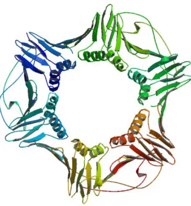
• Quaternary structure: while all proteins contain primary, secondary and tertiary structures, quaternary structures are reserved for proteins which have two or more polypeptide chains, also known as subunits in this context. In proteins with quaternary structures, each polypeptide folds separately and adopts a tertiary structure. Tertiary structures then assemble with each other via intermolecular interactions to form the quaternary structure, also called an oligomer. Depending on the number of subunits, proteins adopt different names. Dimers, trimers, and tetramers are, for instance, proteins composed of two, three and four subunits, respectively. In this sense, a homo-oligomer would be formed by few identical subunits and by contrast, a hetero-oligomer would be made of more than one, different, subunits (see Figure 3).
As enzymes are a special type of proteins, throughout this thesis, we use ‘protein’ and ‘enzyme’ interchangeably. The remainder of the thesis is organized as follows. In Chapter 2, we describe the data and demonstrate how we have preprocessed and curated it to generate our datasets. Chapter 3 lays out the adopted computational approaches that we have investigated to find a fitting model. Chapter 4 deals with a series of experimental setting concerning the employed computational methods. In Chapter 5, we report the results, and discuss our findings in Chapter 6.
Figure 3: An example of a protein quaternary structure consisting of 3 polypeptide chains. PDB ID: 1AXC (www.rcsb.org) [Berman et al., 2000; Gulbis et al., 1996].
Figure 4: An illustration of the 4 level of protein structures. (a) Primary structure: sequence of a chain of amino acids. (b) Secondary structure: local folding of the polypeptide chain into helices or sheets. (c) Tertiary structure: 3D folding pattern of a protein due to side chain interactions. (d) Quaternary structure: protein consisting of more than one amino acid chain. [OpenStax CNX,]
2
Data
The initial data was extracted from the UniProt Knowledgebase (UniProtKB) database [The UniProt Consortium, 2017], a protein database partially curated by experts, by querying a list of all entries with at least one cross-reference to the Protein Data Bank (PDB) database [Berman et al., 2000]. The retrieved list consists of 43,394 unique UniProt IDs, containing both reviewed (manually annotated) and unreviewed (automatically annotated) entries. Thus, the initial dataset was gathered using the information provided for the entries (UniProt IDs) such as proteins’ amino acid sequences, catalytic activities (the chemical reactions proteins catalyze) and pointers to PDB. The dataset was then filtered by selecting those proteins with annotated catalytic activities, or in other terms, Enzyme Commission (EC) numbers [Bairoch, 2000], totaling 14,100 proteins.
2.1
Promiscuity
In order to define promiscuity in a more concrete manner, we followed Khersonsky and Tawfik’s approach, which assesses the degree of promiscuity by comparing differences in the EC numbers [Khersonsky and Tawfik, 2010]. The Enzyme Commission (EC) number systematically classifies and names the enzymes based on the chemical names of the substances they modify (substrates) and the chemical reactions catalyzed by them. Each EC code consists of four numbers separated by periods representing a progressively finer classification of the enzyme as we move from the leftmost number towards the rightmost one. According to Khersonsky and Tawfik, in case of catalytic promiscuity, a protein is annotated with at least two EC codes which differ in the third, second, or even first numbers (which indicates a different reaction category) ignoring the fourth number, whereas multispecificity, or substrate promiscuity, is concerned with differences only in the fourth number.
Focusing solely on catalytic promiscuity and considering Khersonsky and Tawfik’s approach, we split the list into promiscuous (positive) and non-promiscuous (negative) sets containing 688 and 13,412 proteins, respectively.
2.2
Data Preprocessing
Each UniProt ID might have more than one cross-reference to PDB meaning that a number of different structures might be available for each protein. These structures differ for a number of reasons, one of which is having different resolutions. Another reason is that some structures apply to apoproteins (proteins that require a cofactor but do not have one bound) while some others apply to proteins complexed with various ligands. Moreover, different structures can belong to various mutants of the same protein. Similar to UniProt entries, PDB structures can point to different identifiers and databases as well. This information can be found in the DBREF record of PDB files.
Here, we restricted our dataset to having only one cross-reference to PDB per each protein by introducing the following conditions:
1. For each protein, we considered only those PDB structures which have cross-references to its UniProt ID in the DBREF record of their PDB files.
2. We discarded all PDB structures whose resolution is greater than 5Å or lack a reported resolution.
3. In order to select the best PDB structure for each protein, we took into account the completeness of the structures which is examining the number of residues for which 3-dimensional coordinates are provided in the PDB files.
Applying these conditions, we excluded the proteins whose all PDB structures failed to meet the aforementioned conditions, leaving us with 590 and 11,294 promiscuous and non-promiscuous proteins, respectively.
Furthermore, redundancy was removed within each set by clustering the protein sequences at a threshold of 50% of sequence similarity using the CD-HIT program [Huang et al., 2010], and then selecting only one protein per each cluster. This similarity threshold corresponds to the alignment of 3-mers, which are peptides containing three amino-acid residues, called tripeptides. As an additional filter, redundancy in terms of uniqueness of cross-references to PDB has was as well. Also, in an attempt to eliminate the possible noise inflicted mainly by misannotations, overlaps between the promiscuous and non-promiscuous sets was removed by leaving out the proteins which have identical protein sequences, or are annotated with identical sets of EC numbers. This resulted in 406 promiscuous and 7,916 non-promiscuous proteins as the our base set.
2.3
Datasets
Based on the initial data extracted from UniProt along with the pointers to PDB, we formed two individual sets of datasets according to proteins’ different representations (see Figure4).
2.3.1 The Sequence Dataset
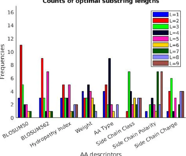
The sequence dataset contains proteins’ linear amino acid sequences, or in other terms, their primary structures, coupled with their physicochemical properties. We study the sequences associated with the UniProt IDs in our base set along with their amino acids’ descriptors, namely residue types, hydropathy indices and weights as well as side chain class, polarity, and charge (see Table1). Moreover, BLOSUM50 and BLOSUM62 substitution matrices are examined as additional amino acid descriptors.
Similar to our base set, we have 406 promiscuous and 7,916 non-promiscuous sequences in our sequence dataset.
AA1 Side Chain Class Side Chain Polarity Side Chain Charge Hydropathy Index Weight
Ala aliphatic nonpolar neutral 1.8 89.0940 Arg basic basic polar positive -4.5 174.2030 Asn amide polar neutral -3.5 132.1190 Asp acid acidic polar negative -3.5 133.1040 Cys sulfur-containing nonpolar neutral 2.5 121.1540 Glu acid acidic polar negative -3.5 147.1310 Gln amide polar neutral -3.5 146.1460 Gly aliphatic nonpolar neutral -0.4 75.0670
His basic aromatic basic polar neutral -3.2 155.1560 Ile aliphatic nonpolar neutral 4.5 131.1750 Leu aliphatic nonpolar neutral 3.8 131.1750 Lys basic basic polar positive -3.9 146.1890 Met sulfur-containing nonpolar neutral 1.9 149.2080 Phe aromatic nonpolar neutral 2.8 165.1920 Pro cyclic nonpolar neutral -1.6 115.1320 Ser hydroxyl-containing polar neutral -0.8 105.0930 Thr hydroxyl-containing polar neutral -0.7 119.1190 Trp aromatic nonpolar neutral -0.9 204.2280 Tyr aromatic polar neutral -1.3 181.1910 Val aliphatic nonpolar neutral 4.2 117.1480
Table 1: Physicochemical properties of amino acids
2.3.2 The 3D Structure Datasets
The 3D structure datasets was gathered using the cross-references to PDB. PDB files often contain information on proteins’ quaternary structures in case of oligomers, or tertiary structures in case of proteins with only one single polypeptide chain. However, sometimes coordinates of only a portion of a protein macromolecule is available in its PDB file. We have constructed 3 different datasets using the 3D coordinates in the PDB files.
• The UniProt-unique-chains dataset: as previously mentioned, a protein can be an oligomer containing more than one chain. However, in the DBREF record of PDB files, not all chains necessarily point to the same ID or even database. For a specific protein with a unique UniProt ID, this dataset takes into account only those chains corresponding to the same UniProt ID. Furthermore, it includes the coordinates of only one copy of each distinctive chain if several identical chains are available.
• The UniProt-all-chains dataset: for each protein, this dataset comprises the coordinates of all the chains associated with its UniProt ID.
• The all-coordinates dataset: the coordinates of all the chains available in the PDB file irrespective of their cross-referenced IDs or databases are included in this dataset.
In order to avoid computational complications, in all the 3D structure datasets, the coordinates of each are represented by the coordinates of its alpha-carbon (Cα) atoms. If the α-carbon coordinates are missing, the coordinates of either the amine group’s nitrogen or the carboxyl group’s carbon atoms are used.
Residue’s secondary structure attributes, which are α-helix and β sheet, and primary structure descriptors, namely residue type, side chain class, polarity, and charge are used as data features.
Similar to our base set, we have 406 promiscuous and 7,916 non-promiscuous proteins in each of the 3D structure datasets. In the following chapter, we will discuss the methods we have employed to analyze these datasets.
3
Methods
We treat the task of predicting the promiscuity status of a protein as a supervised binary classification problem where promiscuous and non-promiscuous proteins form the positive and negative classes, respectively. In a supervised binary classification, there are a set of training instances with known binary classes, and the objective is to find a predictive model which is capable of predicting the classes of unseen data accurately.
In this chapter, we will endeavour to illustrate the computational approaches that we have investigated to find a fitting predictive model. We begin the chapter with discussing a baseline approach. We will then continue with elaborating on kernel methods preceded by a brief description on the type of their learning algorithms. The kernel methods themselves are divided into two groups based on the type of the dataset, namely, the sequence-based or 3D structure-based.
3.1
BLAST
In order to have a reference point for predicting the enzyme promiscuity, we have attempted to classify the unseen data by means of the BLAST algorithm [Altschul et al., 1990; Altschul et al., 1997] as a baseline. BLAST stands for Basic Alignment Search Tool, which is arguably the most heavily used algorithm for annotating and comparing biological sequences such as nucleotides of DNA or proteins’ amino acid sequences quickly and accurately. As there are many possible ways a sequence might align with sequences in a database, searching a large database of sequences can be exhaustive. Blast speeds up this process by conducting local alignments, that is, it looks for small regions of perfect match between the queried sequence and target sequences irrespective of where they are in the sequence. It then investigates the sequence that adjoins these short regions to see whether there is a longer stretch that matches perfectly.
A blast search starts with sets of three-letter words, also called 3-mers, which represent three nucleotides or amino acids in a specific order. It then looks for all common three-letter words between the query sequence and the hit sequences from the database and counts the number of times these words appear. Closely related words, called neighbors, which differ in only one or two letters are examined as well. These neighbors, however, should satisfy a similarity threshold of at leastT according to a scoring matrix. Matches are then found by comparing the assembled words and their neighbors to the sequences in the database.
BLAST is a family of different programs which vary depending on the type of input, the database being searched, and what is being compared [Camacho et al., 2009]. Since we are interested in proteins, we use protein-protein BLAST (blastp) which is a program that for a protein query, returns the most similar protein sequences from a protein database specified by the user. In our classification problem, a protein sequence with unknown label is scanned against a local database formed by the training sequences. We then assign the class label of the hit sequence with the highest similarity score to the new protein.
3.2
Instance-Based Learning
In machine learning, instance-based learning (IBL), sometimes called memory-based learning, refers to a family of classifiers whose main distinctive characteristic is to use the instances themselves as class representations instead of constructing explicit generalizations and abstractions such as decision trees [Quinlan, 1986] or rules. In order to classify unseen instances, IBL algorithms compare new problem instances with instances seen in training, which have been stored in memory. The classification, thus, relies on the similarity between the new observation to be classified and the previously seen instances as the hypothesis is constructed directly from the training instances.
Two examples of instance-based learning classifiers are the k-nearest neighbor algorithm (k-NN) [Cover and Hart, 1967], which we will explain in greater detail later in this chapter (Section 3.3.1.3), and kernel methods [Shawe-Taylor and Cristianini, 2004; Vapnik, 1995]. When predicting a value/class for a new instance, these algorithms compute distances or similarities between this instance and the training instances to make an inference.
3.3
Kernel Methods
Kernel methods are a class of algorithms for pattern analysis, in which the general task is to find and study general types of relations in datasets. In many classification algorithms, the objective is to learn a nonlinear function or decision boundary. To this end, the raw data, which is often non-vectorial, needs to be explicitly transformed into feature vector representations via a user-specified feature map. Strings, graphs and trees are examples of non-vectorial, structured data. Kernel methods, however, offer an alternative which is a single similarity function over pairs of data points in their raw representation without the need for explicit computation of the coordinates in the feature space. This approach , called the "kernel trick", is often computationally cheaper than the explicit computation of the coordinates.
Kernel Trick
The explicit mapping that is needed to get linear learning algorithms to learn a nonlinear function or decision boundary can be avoided by employing the kernel trick. Ifk: X × X →R is a kernel function, for all xand x0 in the input space X,
k(x,x0) can be expressed as an inner product in another space V. In other terms, if
ϕ: X → V is a feature map, thenk(x,x0) =hϕ(x), ϕ(x0)iV. Hence, any linear model
has the potential to be converted into a non-linear model by applying the kernel trick which replaces the features by a kernel function.
Kernel methods can be seen as instance-based learners in that instead of learning fixed parameters corresponding to the features of their inputs, they make predictions for the labels of the unseen data, which are not in the training, according to the kernel values computed between the unlabeled input x0 and each of the training inputsxi ∈ X. A kernel matrix for an input space X with n examples is obtained
In other words, the kernel matrix Kn ∈ Rn×n is a symmetric n×n square matrix
with entries
[Kn]ij =k(xi,xj). (1)
There are numerous algorithms which are capable of operating with kernels such as kernel perceptron, support vector machine (SVM) [Cortes and Vapnik, 1995], Gaussian processes (GP) [Williams and Rasmussen, 1996; Neal, 1996], principal components analysis (PCA), canonical correlation analysis (CCA), and ridge regression, to name a few. In this study, as the binary classification tool, we employ SVM, which is an effective model used for the same purpose.
Support Vector Machine
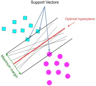
In a binary classification, the key idea of the Support Vector Machine is to construct a hyperplane which could successfully split the high-dimensional data points which are linearly separable into two classes. As there might be a large set of different hyperplanes separating the two classes, intuitively, a good separation is achieved by the hyperplane which has the maximum distance to the closest data points of either class. These data points are referred to as support vectors and the distance from the hyperplane to them is called margin (see Figure 5).
Figure 5: An intuition for the main idea behind Support Vector Machine. For a specific decision hyperplane, the linear discriminant function can be formu-lated asf(x) =wTx+b, wherexis a data point,wis the decision hyperplane normal
vector which is perpendicular to the hyperplane, and b is an intercept term. The class assignment is then given by y= sign[f(x)], where y∈ {−1,1}. Accordingly, the functional margin of a data point xi with respect to the hyperplane is defined as
the quantity γ(x) =yif(x), whereyi tells in which side of the hyperplane the data
SVM insists on a large margin around the decision boundary. However, one can increase the margin without limit by scaling up w. In order to circumvent this problem, we can impose a scaling constraint which is fixing the margin to γ = 1 and seeking for the shortest weight vector which fulfills this margin. This leads to the following constrained optimization problem:
min w,b 1 2kwk 2 s.t. yi(wTx+b)≥1. (2) This is called the hard margin SVM where constraints ensure that there are no missclassified examples, which is possible since we assumed that the data is linearly separable. However, in practice, data is seldom linearly separable; and even if it is, a greater margin can be achievable by allowing the margin to make some mistakes. To allow errors, we modify the inequality constraints in Equation2and reformulate it as
min w,b,ξ 1 2kwk 2+CX i ξi s.t. yi(wTx+b)≥1−ξi, ξi ≥0, (3)
where ξi ≥0 are slack variables that allow an example to have a smaller margin than
γ = 1, and even to be misclassified, subject to a penalty depending on how far it is from meeting the margin. However, we would like to minimize the sum of the slacks in order to have as few misclassifcations as possible. C > 0 is a constant which controls the trade off between maximizing the margin and the amount of slack needed. The formulation is called the soft-margin SVM which was introduced by Cortes and Vapnik [Cortes and Vapnik, 1995]. Using the method of Lagrange multipliers, we can formulate the Equation3 as a dual optimization problem expressed in terms of variables αi: max αi X i αi− 1 2 X i X j αiαjyiyjxTi xj s.t. X i yiαi = 0, 0≤αi ≤C. (4)
The dual formulation, which gives the same solution to the soft-margin SVM, leads to an expansion of the weight vector in terms of the input examples:
w=X
i
yiαixi. (5)
If the classes cannot be separated linearly, we need to transform the data via some transformationϕ: x→ϕ(x) on to a higher dimensional space where we can use a linear classifier. Following this mapping, Equation 6can be given by
w=X
i
and consequently, substituting it in Equation 4 yields: max αi X i αi− 1 2 X i X j αiαjyiyjϕ(xi)Tϕ(xj) s.t. X i yiαi = 0, 0≤αi ≤C. (7)
According to Section 3.3, by means of the kernel trick, we can replace the inner productϕ(xi)Tϕ(xj) with a kernel functionk(xi,xj), which makes the computations
considerably simpler. SVM is an example of a convex optimization problem which can be solved with the help of existing off-the-shelf efficient algorithms.
This will set the scene for the subsequent sections where we describe the kernels we have employed in this study based on the type of dataset.
3.3.1 Sequence-Based Kernels
Traditional approaches for determination of similarity between two protein sequences begin with strings of letters (amino acids) that represent the sequences. Therefore, in this study as for the proteins sequence dataset discussed in Section2.3.1, we have adopted string kernels [Watkins, 1999; Haussler, 1999], a family of kernel functions designed for sequences. String kernels have applications in text mining and gene analysis where sequence data are to be clustered or classified.
String Kernels
The basic idea of string kernels is to compute the similarity between two strings, which are finite sequences of symbols and can be of different length, without explicitly extracting the features. SVM allows string kernels to work with strings, without having to translate these to fixed-length, real-valued feature vectors. The more subsequences with similar features two strings have in common, the more similar they are considered and thus, the higher value of the kernel function. There are numerous types of string kernels depending how the subsequences are defined. Subsequences can be contiguous or non-contiguous, they can have bounded or unbounded length, and gaps and mismatches can be taken into account subject to different ways of penalization. k-spectrum kernel [Leslie et al., 2002], gap-weighted subsequence kernel (GWSK) [Lodhi et al., 2002], weighted all-substrings kernel (WASK) [V. N. Vish-wanathan and Smola, 2003], and generic string (GS) kernel [Giguère et al., 2013] are among examples of string kernels. In the following, after a brief clarification of some of the notations related to string kernels, we will elaborate upon the k-spectrum and generic string kernels. All the kernels described in this chapter are intended to be evaluated by SVM, however, we will further assess the generic string kernel by utilizing thek-NN method.
String Kernel Notations
Σ = {σ1, . . . , σn}, n ∈ N denotes a finite alphabet of n characters over which the
strings are defined. The kleene star of Σ is denoted by Σ* which is the set of all finite strings formed by characters in Σ. Therefore, a string over Σ can be written as a sequence x=x1x2. . . x|x| which is a concatenation of characters from the alphabet:
xi ∈ Σ for i = 1, . . . ,|x|, where |x| denotes the length of string x. A substring of
string x is a string ˆx = xi+1. . . xi+l where 0 ≤ i and i+l ≤ |x|. We denote all
substrings of length k by Σk.
3.3.1.1 The k-Spectrum Kernel
Given two sequences, x and x0, the k-spectrum kernel, presented in [Leslie et al., 2002], counts the number of substrings of length k in two sequences. The feature vector for each string x is φk(x) which is indexed by substrings of lengthk:
φku(x) =|{(v1, v2) :x=v1uv2}|, u∈Σk, (8)
where each feature φk
u(x) counts for occurrences of a substring.
Therefore, the kernel is defined as
Kk(x, x0) =hφk(x), φk(x0)i= X
u∈Σk
φku(x)φku(x0). (9)
3.3.1.2 The Generic String Kernel
In this study, special attention has been given to the generic string kernel presented in [Giguère et al., 2013], an effective kernel on biosequences. The elegance of the generic string kernel lies in the fact that it builds on several ideas:
• Bounded-length subsequence: it computes kernels over different-length subse-quences up to a length L.
• Position dependency: discrepancies in substring positions are penalized by a Gaussian kernel on the starting indices of the compared substrings.
• Factorized representations: using an encoding functionψ: Σ→Rd, each symbol
ain the alphabet is represented as a feature vectorψ(a) = (ψ1(a), ψ2(a), . . . , ψd(a)),
also called a descriptor, where each ψi(a) encodes one of the d properties of a.
Subsequently, the encoding function ψl: Σl →
Rdl generates the feature vector
of a substring of lengthl asψl(a
1, a2, . . . , al) = (ψ(a1), ψ(a2), . . . , ψ(al)), which
is a concatenation of the feature vectors of l symbols, each ofd components.
• Soft matching: a Gaussian kernel is computed over the squared Euclidean distance between the feature vectors of two subsequences.
The kernel is formulated as KGS(x, x0, L, σp, σc) = L X l=1 |x|−l X i=0 |x0|−l X j=0 e −(i−j)2 2σ2p e −kψl(xi+1,..,xi+l)−ψl(x0j+1,..,x0j+l)k2 2σ2c , (10)
where L≤ is the maximum length for substring comparison,σp is a parameter which
controls the penalty for position differences, and σp is a parameter controlling the
amount of penalty incurred when the squared Euclidean distance between the vectors
ψl(x
i+1, .., xi+l) and ψl(x0j+1, .., x
0
j+l) differs.
3.3.1.3 k-NN
k-NN [Cover and Hart, 1967], a type of instance-based learning discussed in Section
3.2, is one of the simplest classification and regression algorithms. It is a lazy non-parametric method that does not make any assumptions on the underlying data distribution. In a classification task, where the data points are separated into several classes, thek-NN algorithm classifies a new point by a majority vote of its k
nearest neighbors, that is, the class most common among them. 1-NN is the simplest variation of the k-NN algorithm where k = 1. The 1-NN algorithm simply assigns the new point to the class of its closest neighbor. There are different approaches how to define a distance metric for measuring the closeness between two data points. Euclidean distance is the most commonly used distance measure which is defined as
D(x,x0) = kϕ(x)−ϕ(x0)k=qhϕ(x), ϕ(x)i+hϕ(x0), ϕ(x0)i −2hϕ(x), ϕ(x0)i.
(11) By exploiting the kernel trick we can reformulate the Equation 11as
D(x,x0) =qk(x,x) +k(x0,x0)−2k(x,x0), (12)
where k can be any kernel. In this study, we use the 1-NN algorithm and consider the generic string kernel discussed in Section 3.3.1.2for computing the distances in Equation12. Therefore, for each new instance x0 to be classified, we construct the generic string kernel kgs(x,x0) between the new instance and all the instancesx in
the input data space X whose labels are known. The class label of the new data point x0 is then determined by the class of the instance whose distance tox0 is the smallest.
The remainder of this chapter is devoted to detailing the kernels which are adopted for the 3D structure datasets.
3.3.2 3D Structure-Based Kernels
One of the present challenges is to sort out similarities in protein structures in order to gain insight into their functions and characteristics. Previous methods to predict protein characteristics mainly relied on identifying similarity in sequence or structure between a protein of unknown attribute and one or more well-understood proteins [C Whisstock and M Lesk, 2003]. These methods require explicit trans-formation of protein structures into feature vectors, called topological descriptors, which often suffer from not preserving the rich topological information embedded in structures. Moreover, computation of these explicit topological descriptors can be computationally expensive. Therefore, to avoid this loss of information as well as the problem of explicit feature vector transformation, protein structures can be modeled as graphs and subsequently, graph kernel functions can be employed to measure the structural similarities between them. Graph kernels are efficient to compute as they compare substructures of graphs that are computable in polynomial time. Additionally, they allow us to use any kernel-based machine learning method on them. Besides bioinformatics and chemoinformatics, graph kernels find applications further afield in social network analysis, computer vision, and natural language processing. At its most basic, a graph can be defined as a set of 2D or 3D entities and relationships that function in some interrelated way. Therefore, the 3D nature of proteins’ tertiary or quaternary structures and the complex relationships in their polymers enable them to be represented as graphs by means of different mapping rules.
After introducing some of the most important concepts of graph theory, we will continue the chapter with detailed explanations how to model a protein as a graph as well as describing different and state-of-the-art graph kernels.
Graph Theory Concepts
A graph G= hV, Ei consists of a set of vertices V ={v1, v2, . . . , vn} and edges E,
where E ⊂ V ×V. An edge e ∈ E connects a pair of vertices u, v ∈ V, and is denoted ase = (u, v). Vertices u, v ∈V are said to be neighbors or adjacent if they are connected by an edge, that is, if e = (u, v) ∈ E. Accordingly, we define the adjacency matrix of a graph G=hV, Ei as An×n = [aij] wheren is the number of
nodes in the graph Gand aij = 1 if (vi, vj) is an edge of G, and 0 otherwise.
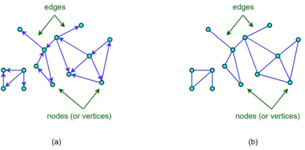
We call a graph attributed or labeled when there are labels on nodes, edges, or both. Labels can be scalars or vectors with either discrete or continues values. A graph is called directed when the edges in E are ordered pairs of vertices, and undirected when they do not have a particular order or direction, i.e. the edge (u, v) is identical to the edge (v, u) (see Figure 6). A graph is simple and self-loop free if there is no edge connecting a vertex to itself and there are no multiple edges connecting the same pair of vertices.
Figure 6: Examples of (a) a directed graph and (b) an undirected graph. A walk of length k in graph Gis a nonempty sequence of vertices v1, v2, . . . , vk
connected by edges e1, e2, . . . , ek−1 such that ei = (vi, vi+1) for all 1 ≤ i < k. w is
called a pathp in Gif the vertices in the sequence are all distinct (see Figure 7). We can also say that a graph G is connected if there is a path between every pair of distinct vertices in G, and disconnected otherwise. Examples in Figure6and Figure
7 are disconnected and connected graphs, respectively.
Figure 7: Examples of (a) a walk and (b) a path between verticesvi and vj.
H =hVH, EHi is a subgraph of G (orH has an embedding in G) with V(H)⊆
V(G) and E(H)⊆E(G), denoted byH vG. A graph is called a tree when any two vertices are connected by exactly one edge, resulting in a connected structure with no cycles. Therefore, a (rooted) subtree is an acyclic subgraph of a graph which has a designated root. The height of a subtree is then defined as the longest path between the root and any other node in the subtree. Subtree patterns allow repetitions of nodes. However, in order to avoid cycles, they treat the repetitions of the same node as distinct nodes (see Figure 8).
For two graphs G = hV, Ei and G0 = hV0, E0i, isomorphism is defined as a
bijective mappingf :V →V0 such that (vi, vj ∈E) if and only if (f(vi), f(vj))∈V0.
Figure 8: An example of a a subtree pattern of height 2 rooted at the node 1 where repetitions of nodes are allowed. [Shervashidze et al., 2011]
Proteins as Graphs
The structure of a protein is mainly governed by its residual interactions, peptide bonding, covalent interactions, and hydrophobic packing. Depending on the type of interaction, proteins can be mapped to topologically different graphs. When modeling a protein as a graph, one can define the vertex set based on different aspects of protein structures. Examples include residues [Samudrala and Moult, 1998], side chains [Canutescu et al., 2003], Cα atoms [Huan et al., 2005], SSE (secondary structure elements) [Borgwardt et al., 2005], and DSSP (the dictionary of protein secondary structures) [Peng and Tsay, 2010]. As for the edge set, usually the distance of two vertices with some labels, e.g., chemical properties, is translated into an edge between them. A pictorial overview of protein graph remodeling is depicted in Figure9.
Figure 9: An overview of protein graph remodeling. [Peng and Tsay, 2014] In this study, we model the proteins such that they contain information on their structures, sequences and chemical properties. To this end, we design our models as simple attributed and undirected graphs having no self-loops. Each graph corresponds to exactly one protein. Among different elements previously discussed to construct the vertex set, we opt for Cα atoms and consider edges between them if they are within a sphere of 5Å. In other terms, for each pair of Cα atoms, we measure the Euclidean distance between their 3D coordinates and assign an edge between them
only if the distance is smaller than 5Å. We do not consider any labels for the edges. However, vertices bear single-valued labels. We try different node attributes, namely secondary structure elements, i.e. helices, sheets or unknown, amino acid types, side chain classes, polarity statuses, and charge attributes. Details of these categorical features can be found in AppendixA. We follow the same approach for all the three 3D structure datasets discussed in Section 2.3.2.
Graph Kernels
The basic idea of graph kernels is to count common substructures in two graphs. Given two graphs G and G0 from the space of graphs G, the problem of graph comparison is defined as finding a mapping s:G × G →R such that the similarity of G andG0 can be quantified as s(G, G0). A mapping satisfying the conditions of symmetry and positive definiteness is called a graph kernel. Many of the existing graph kernels are instances of the family of so-called R-convolution kernels [Haussler, 1999] which is a generic framework for defining kernels on discrete compound objects decomposed into smaller components. All pairs of decompositions, or subgraphs in other words, are then compared. In consequence, different types of decomposition relationsR result in different graph kernels. The main purpose of convolution kernels is to make the comparison less difficult by means of defining and computing a simpler similarity measure over the smaller, less complex subgraphs. However, comparing all the decomposed subgraphs is at least as hard to compute as deciding if two graphs are isomorphic [Gärtner et al., 2003] which leads to restricting graph kernels to compare only specific types of subgraphs that are computable in polynomial time. The family of R-convolution kernels can be grouped into the following categories, namely graph kernels based on comparing all pairs of decomposed random walks [Gärtner et al., 2003;Kashima et al., 2003; Mahé et al., 2004; Vishwanathan et al., 2006], shortest paths [Borgwardt and Kriegel, 2005], cycles [Horváth et al., 2004], limited-size subgraphs (graphlets) [Borgwardt et al., 2007; Shervashidze et al., 2009], and subtree patterns [Ramon and Gärtner, 2003;Mahé and Vert, 2009;Shervashidze and Borgwardt, 2009; Shervashidze et al., 2011; Neumann et al., 2012; Feragen et al., 2013]. Most of these kernels suffer from poor scalability to large, labeled graphs containing more than 100 nodes. In this study, we have investigated two graph kernels which are scalable to large graphs: the graphlet kernel proposed by [Shervashidze et al., 2009] and the Weisfeiler-Lehman graph kernel, a state-of-the-art subtree kernel presented in [Shervashidze et al., 2011].
3.3.2.1 The Graphlet Kernel
The key idea of the graphlet kernel [Shervashidze et al., 2009] is similar to that of the
k-spectrum kernel discussed in Section 3.3.1.1 with a difference that in the graphlet kernel, the value of k is bounded. The graphlet kernel compares the frequencies of all types of subgraphs of size k ∈ {3,4,5} in two unlabeled graphs. These subgraphs are referred to as graphlets [Pržulj, 2007]. IfGis a graph withnnodes, let
the number of occurrences of subgraph(i) in G by #(graphlet(i)vG). The vector
fG of length Nk, called the k-spectrum vector, can be defined as
fGi = #(graphlet(i)vG). (13)
The graphlet kernel kg over two graphs G and G0 then takes the form:
kg(G, G0) = fGTfG0. (14)
Since the differences in the sizes of the graphs can greatly skew the frequency counts
fG, counts are normalized to probability vectors:
DG=
1
#all graphlets in GfG, (15)
and therefore, the graphlet kernel can be reformulated as
kg(G, G0) = DGTDG0. (16)
In order to reduce the expensive runtime of computing all the graphlet distribu-tions, two speedup schemes are employed which are based on graphlet sampling and the limitation of bounded degree graphs. According to the sampling scheme, if the number of samples achieves a given confidence with a small probability of error, then the empirical distribution is close to the actual distribution of the graphlets. The scheme based on the exploitation of the low maximum degree of graphs states that if
d denotes the maximum degree of a graph, then the exact number of all graphlets of size k∈ {3,4,5} in a bounded graph G can be enumerated in O(ndk−1) time, where n is the number of nodes in G.
In this project, we only consider graphlets of size 3 (see Figure 10).
3.3.2.2 The Weisfeiler-Lehman Subtree Kernel
The Weisfeiler-Lehman (WL) subtree kernel [Shervashidze et al., 2011] is an efficient kernel which can scale to large graphs with thousands of both unlabeled and discretely labeled nodes. It encompasses many of the previously known graph kernels and in graph classification tasks, is competitive with or outperforms other state-of-the-art graph kernels. The general framework for the WL graph kernels is constructed according to the Weisfeiler-Lehman test of isomorphism which is used to determine whether two graphs are isomorphic.
The Weisfeiler-Lehman Test of Isomorphism
For two graphsGandG0, the Weisfeiler-Lehman test algorithm proceeds in iterations, each of which consisting of a sequence of steps. In every iteration, the label of each node is augmented by the sorted set of node labels of its neighbouring nodes, called a multiset. These augmented labels are then compressed into new, short labels. Figure
11depicts an illustration of these steps in the first iteration of the algorithm.
Figure 11: An illustration of the first iteration of the Weisfeiler-Lehman test of isomorphism [Borgwardt and Stegle, 2010].
Relabeling of the nodes with compressed, new labels in the last step is concordant inGandG0, meaning that they will get identical new labels only if they have identical multiset labels. The Weisfeiler-Lehman algorithm terminates after this step if the number of iterations reaches n, or if the node label sets of Gand G0 start to diverge, that is, if the sets of newly created labels are not identical in G and G0. After n
iterations, if the sets are identical, two cases are possible:
• eitherG and G0 are isomorphic in fact, or
The Weisfeiler-Lehman Kernel Framework
In this context, a graphGis defined as a triplet (V, E, l) wherel: V →Σ is a mapping function which assigns labels from an alphabet Σ to the graph nodes. According to the WL algorithm, each node v gets a new labeling li(v) in each iteration i.
Therefore, one iteration of the WL algorithm can be defined as a relabeling function
r((V, E, li)) = (V, E, li+1) which transforms all the graphs in a set of graphsG in the
same manner. The compressed labels li(v) in iteration i can be considered a subtree
pattern of heighti rooted atv (see Figure 8for an illustration of subtree patterns). If Gi = (V, E, li) is the Weisfeiler-Lehman graph at height i of the graph G =
(V, E, l) = (V, E, l0), the sequence of Weisfeiler-Lehman graphs up to height h of G
is then given by
{G0, G1, . . . , Gh}={(V, E, l0),(V, E, l1), . . .(V, E, lh)}, (17)
where G0 =G, l0 =l and Gi =r(Gi−1).
Having defined the sequence of Weisfeiler-Lehman graphs, we can formulate the general Weisfeiler-Lehman kernel on two graphsG and G0 with h iterations as
k(W Lh)(G, G0) = k(G0, G00) +k(G1, G01) +. . . , k(Gh, G0h), (18)
where k(., .) is a base kernel and {G0, . . . , Gh} and {G00, . . . , G
0
h} are the
Weisfeiler-Lehman sequences of G and G0 up to height h, respectively.
The Weisfeiler-Lehman subtree kernel is an instance of the general WL kernel (Equation20) that compares subtrees of height h in two graphs. The base kernel k
of the WL subtree kernel is a function which counts pairs of matching node labels in two graphs Gand G0 given by
k(G, G0) = X
v∈V X
v0∈V0
δ(l(v), l(v0)), (19)
where δ is the Dirac kernel, which is 1 when the labelsl(v) andl(v0) are equal, and 0 otherwise. In other terms, the Weisfeiler-Lehman subtree kernel adds up the common labels in two graphs counted in each iterationi∈ {0,1, . . . , h}. Thus, it can be also expressed as
kW Lsubtree(h) (G, G0) =hφ(W Lsubtreeh) (G), φ(W Lsubtreeh) (G0)i, (20) where φ(W Lsubtreeh) is a feature vector whose components correspond to the frequency of occurrences of common original and compressed labels in two graphsGand G0 up to a height h (see Figure 12for an illustration).
Figure 12: Illustration of the computation of the Weisfeiler-Lehman subtree kernel for height h= 1 [Shervashidze et al., 2011].
4
Experimental setting
This chapter is concerned with a series of experiments and their setups conducted to evaluate the performance of the methods discussed in Chapter 3, which address the problem of protein promiscuity classification.
4.1
Performance Measures
In a binary classification, there are 4 types of predictions:
• True Positive (TP): instances correctly classified as positive
• False Positive (FP): instances incorrectly classified as positive
• True Negative (TN): instances correctly classified as negative
• False Negative (FN): instances incorrectly classified as negative.
Confusion matrix, which is constructed according to the above-mentioned definitions, is a clean and unambiguous way to present and summarize the prediction results of a classifier (See Figure13).
Figure 13: Confusion matrix.
In machine learning, there are different metrics for measuring the performance of a classifier. In order to assess and compare the different methods, we have utilized the following measures defined based on the confusion matrix:
Accuracy: the most intuitive and natural measure to evaluate a classifier on a set of test data is accuracy defined as the number of correct predictions the classifier has achieved divided by the total number of observations in the test set.
Accuracy = T P +T N
Precision: the ratio of correctly predicted positive observations to the total predicted positive observations is called precision.
P recision= T P
T P +F P (22)
According to Equation 22, if all the test instances have been predicted as negative, the denominator becomes zero. We have reported these precisions as N/A in the next chapter.
Recall: the ratio of correctly predicted positive observations to the all observations in the positive class is called precision.
Recall = T P
T P +F N (23)
F1 Score: in case of imbalanced datasets, where the samples from one of the classes outnumbers the other, the accuracy determined using Equation 21may not be an adequate measure of performance. Moreover, accuracy is not capable of capturing the effectiveness of a classifier when the performance of one of the classes in particular is of interest. Compared to the above 3 metrics, the F1 score provides a more balanced view. It is defined as the weighted average of precision and recall.
F1 Score= 2∗(P recision∗Recall)
P recision+Recall (24)
Acquiring a high precision, but low recall indicates that the predictor is quite reliable and sensitive not to make mistakes in labeling the negative examples incor-rectly as positive. This means that the positive portion of the predictions can be safely assumed as actually positive. However, the classifier has not been successful in detecting most of the positive examples.
The opposite scenario, when the precision is low, but a high recall is achieved suggests that the classifier is capable of identifying most of the positive examples, while it is not reliable whether a positive-labeled example is actually positive.
Low precision and low recall, on the other hand, means that the classifier’s performance in identifying actual positive instances has been quite poor. This results in a low F1 score as well.
High values for both precision and recall are achieved when the classifier has been able to accurately identify both of the negative and positive classes accurately. This scenario leads to a high F1 score.

![Figure 9: An overview of protein graph remodeling. [Peng and Tsay, 2014]](https://thumb-us.123doks.com/thumbv2/123dok_us/1991407.2795876/27.892.151.788.666.869/figure-overview-protein-graph-remodeling-peng-tsay.webp)
![Figure 11: An illustration of the first iteration of the Weisfeiler-Lehman test of isomorphism [Borgwardt and Stegle, 2010].](https://thumb-us.123doks.com/thumbv2/123dok_us/1991407.2795876/30.892.172.761.492.776/figure-illustration-iteration-weisfeiler-lehman-isomorphism-borgwardt-stegle.webp)
![Figure 12: Illustration of the computation of the Weisfeiler-Lehman subtree kernel for height h = 1 [Shervashidze et al., 2011].](https://thumb-us.123doks.com/thumbv2/123dok_us/1991407.2795876/32.892.172.754.291.830/figure-illustration-computation-weisfeiler-lehman-subtree-kernel-shervashidze.webp)