Practical OCR system based on state of art neural networks

Bachelor’s Thesis

Czech

Technical

University

in Prague

F3

Practical OCR system based on

state of art neural networks

/ Declaration

Prohlašuji, že jsem předloženou práci vypracoval samostatně a že jsem uvedl veškeré použité informační zdroje v souladu s Metodickým pokynem o do-držování etických principů při přípravě vysokoškolsckých závěrečných prací.

Abstrakt / Abstract

Character Recognition) je kýženým cí-lem. Na dosažení tohoto cíle bylo vyna-loženo v průběhu desetiletí značné úsilí. V současnosti je tento problém poklá-dán za více méně vyřešený, vzhledem k tomu že na první pohled dnes OCR fun-guje relativně dobře. Bohužel, při bliž-ším pohledu se ukazuje, že momentálně dostupné nástroje spoléhají na kontrole výstupu za pomoci slovníku, případně jazykových modelů. Toto těmto nástro-jům umožňuje porovnávat různé prav-děpodobné interpretace vstupních dat s ohledem na to, jaké výstupy jsou nej-pravděpodobnější na základě toho zda dávají jazykově smysl. Výkonnost těchto nástrojů je ale na nejazyčných datech jako jsou různé alfanumerické kódy pod-statně horší. Tato práce se pokouší o im-plementaci struktury datasetu, syntetic-kého generátoru dat pro výrobu realis-tických trénovacích dat, a konečně o im-plementaci klasifikátoru na bázi strojo-vého učení schopného fungovat na neja-zykových datech lépe než momentálně dostupná řešení.

Optical Character Recognition has been recognised as a desirable task since long ago, with much engineering effort put towards its solution over the span of decades with the current general con-sensus considering it to be a more or less “solved” as a problem as by most obvi-ous metrics OCR has been performing well for a long time. At closer inspec-tion of attainable performance with the currently available tools, it turns out that they generally rely on cross referencing results obtained from the visual data with a dictionary or some sophisticated linguistic model. This allows them to probabilistically evalu-ate various interpretations of the visual input and ensure data sanity. Their performance on non-linguistic data like codified alphanumerical strings is sig-nificantly worse. This work attempts to implement a dataset structure, a syn-thetic data generator for the generation of realistic training data and ultimately a deep neural net based classifier capa-ble of outperforming availacapa-ble tools in non-linguistic text recognition.

/ Contents

3 OCkRE OCR Implementation . . . 5

3.1 Model input and output . . . 5

3.2 Structural overview . . . 6

3.3 The deep net classifier . . . 6

3.3.1 Convolutional stage . . . 7

3.3.2 Recurrent stage . . . 8

3.3.3 Auxiliary structures . . . 9

3.3.4 Output of the deep classifier . . . .10

3.4 Optimizer . . . .11

3.4.1 SGD . . . .11

3.4.2 Adam . . . .12

4 . . . .13

4.1 Dataset of the original Keras example . . . .13

4.2 Real data extraction and handling in OCkRE . . . .13

4.3 Synthetic data generation . . . . .14

4.3.1 Strings . . . .14 4.3.2 Text bitmaps . . . .14 4.4 Visual augmentations . . . .14 4.4.1 Speckle . . . .15 4.4.2 Line noise . . . .15 4.4.3 Blur . . . .16 4.4.4 Clouding . . . .16

4.4.5 Contrast and inversions . 16 4.4.6 Compounding . . . .17

5 Means of evaluation . . . .18

5.0.1 CTC Loss . . . .18

5.0.2 Mean Normalized Edit Distance . . . .18

5.0.3 Label Accuracy . . . .18

6 Evaluation of achieved perfor-mance. . . .19

6.0.1 Performance in com-parison with Tesseract . . .19

7 Conclusion . . . .20

A Attached files . . . .21

Chapter

1

Introduction

ABBYY; one of the leading companies in commercial OCR products and services, de-fines OCR as follows [[1]:“Optical Character Recognition, or OCR, is a technology that enables you to convert different types of documents, such as scanned paper documents, PDF files or images captured by a digital camera into editable and searchable data.” In other words, OCR is a tool or service capable of comprehending visualinput (usually in form of a bitmap image) as text in a format encoded by a character set. This is necessary for further digital processing of the information within the text, be it in for the purpose of a full-text search, use in database queries or just archiving of the infor-mation in a more compact format. As Adnan Ul-Hasan wrote in his 2016 PhD thesis [2](Abstract), “The task of printed Optical Character Recognition (OCR) is considered a “solved” issue by many Pattern Recognition (PR) researchers.” The performance on many kinds of document appears very good, even with the old methods, on many type-faces and formats of writing. He however further expands on the idea that while the problem is generally considered to be solved, it only appears to be true in case of text written in the commonly used languages and scripts. He largely focuses on the possi-bilities of developing a highly accurate OCR even for less commonly examined scripts and languages. The research paper “Can we build language-independent OCR using LSTM networks?” [3] (co- authored by Adnan Ul-Hasan and Thomas Breuel) begins with “Language models or recognition dictionaries are usually considered an essential step in OCR. However, using a language model complicates training of OCR systems, and it also narrows the range of texts that an OCR system can be used with.” This outlines the issue with the claim that OCR is a “solved” problem.Common OCR sys-tems work well only as long as it’s possible to rely on cross reference from a dictionary and/or a language model. There are however many cases where dictionary inference and language model modeling isn’t practical or possible.The particular case for which this work attempts to develop improved OCR is reading of alphanumerical strings which serve as various IDs, reading of dates or reading of numerical amounts. The use case for our work is as an internal part of a more complex data processing pipeline meant to perform data extraction from structured documents.Both Adnan Ul-Hasan’s thesis and the earlier research paper strongly propose utilisation of LSTM (Long-short term memory) deep nets, as these deep learning classifiers display ability to operate well even in absence of dedicated, detached and specialised dictionary or language model to infer from. This is why our OCR implementation builds on a very similar architecture.

1.1

Historical summary

As Line Eikvil writes in his work “OCR - Optical Character Recognition”[4], the very first technological developments that had something to do with OCR can be traced all the way back to end of the nineteenth century, namely the invention of mosaic photocell scanner invented by C.R.Carey in 1870 and then still before the end of that century, the Nipkow disc, allowing sequential scanning of a visual object.As he continues, the

1. Introduction

. . . .

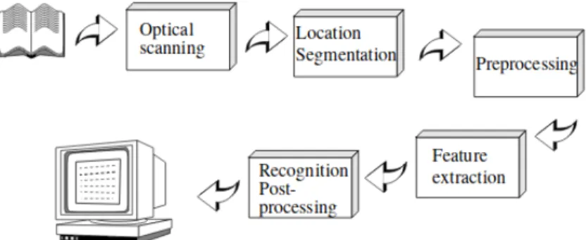
first true OCR machines came sometime in 1950s, with first commercial use becoming feasible in first half of 1960s.The lastly named period is further called the “first genera-tion OCR” distinguished by the explicit specialisagenera-tion of each such machine on just one typeface or just a few of them, with each additional typeface requiring specific set of matching data in the machine’s memory.The second generation which came afterwards was distinct in ability to recognise any regular typeface, with limited attempts to also recognise handwritten text. As described by Line Eikvil, the third generation of OCR coming in the middle of 1970 was specific in much greater reliability and accessibility, making it feasible to use typewriter as a prototyping of sorts, before the documents got ultimately processed digitally, which was still of a great cost, at the time. Important distinction that further connected all the generations of OCR as seen by Line Eikvil was the idea of the inherent layout of such as displayed in Figure 1.1, as shown in Eikvil’s work.

Figure 1.1. The infographic well summarises the core functions of the OCR of the time. The differences from this concept will be juxtaposed on later in this work.

Chapter

2

Current situation

As with many previously purpose built machines and systems, while there is still spe-cialised products including hardware (for instance products of the company Scancorpo-ration [5]), OCR is today largely available as complementary software for image scan-ning devices like page scanners [6], but is also very well accessible as purely software based solution, with many free, open source tools available, as presented for instance by the Ubuntu distribution manual page reserved for OCR [7]. As the lastly named manual page states, one of the most accurate OCR tools is Tesseract, which this work will further focus on as the baseline technology for evaluation of current OCR capability on basis of its relatively high performance and open source, free nature.

2.1

Tesseract

As Ray Smith states in his Overview of the Tesseract OCR Engine [8], Tesseract be-gan life as a private venture of HP, beginning in 1984 and first appearing publicly in 1995. At this point in history, it astounded with at the time very impressive accu-racy and practical capability. In 2005, HP released Tesseract as open source, and it has been acquired by Google which re-released it in 2006, sponsoring its research since then. The cited overview however spoke of the situation back in 2007, situation which has markedly changed with the alpha of Tesseract 4.0, which became public in very early 2017. The main distinguishing feature of Tesseract 4.0 as presented by the 2016 presentation Building a Multi-Lingual OCR Engine [9] by Ray Smith of Google Inc is improvement over the current accuracy achieved by transition to the LSTM based classifier [10]. The presentation promises Tesseract 4.0 accuracy in high 90

2.2

Current apparatus

Our work has started within the previously set requirements of a document reading pipeline currently in active development.The goal of the broader project, called Mor-gan, is to parse information of interest from structured documents, for now particularly invoices. The idea is that the user presents the Morgan API with a PDF document (for instance, an invoice) with or without a text layer to it. The API is meant to be able to autonomously seek out information of interest like the account numbers, dates, and monetary amounts, returning them in a database friendly format.The OCR classifier of this work has been so far integrated as the final stage OCR, applied on cutouts of already pinpointed information of interest, with some degree of functional success.The previous ad hoc solution involves use of the Tesseract OCR engine installed in a Linux environment. Tesseract OCR is generally available in the form of source code,as well as pre-compiled packages [11]. The Tesseract tool lacks a graphical user interface and relies on manipulation either within the command line shell or calls into the C++ API provided by the Tesseract libraries. Past installation, Tesseract is immediately usable

2. Current situation

. . . .

for OCR work, accepting PNG files as input and providing output either in the form of a new textfile or by using “stdout” functionality of the command shell. It is also capable of producing a PDF document, with a searchable, invisible text layer overlaid over the original raster image.

Chapter

3

OCkRE OCR Implementation

This work’s implementation of OCR is based on a single end-to-end neuralnet based classifier. The original design of the classifier, as well as some of the training and evaluation infrastructure is based on an example provided by the open source Keras project [12]. The software module product of this work has been named OCkRE and will be called as such through the rest of this work to distinguish which parts of the final product are original and unmodified part of the example, and which have been changed, modified or added to better suit our use case and to enhance the performance on the OCR task. As its provenance of beginning as a Keras example hints, OCkRE works wholly as a module written in the Python programming language, most criti-cally depending on the Keras deep learning library itself.For practical use of the OCR, all what’s needed is a single Python module and a file with the weights of the neural net classifier with some auxiliary libraries installed in the system, most crucial obvi-ously being Keras itself. The training-ready structure relies on a somewhat broader array of modules, primarily the dataset handling structure.Although the Keras library hopes to be compatible with both Tensorflow[13] and Theano[14] libraries, our work has only been developed and tested with the Tensorflow backend and it’s quite possible it wouldn’t operate well with Theano,particularly due to the specialities of CTC loss calculation.

3.1

Model input and output

OCkRE operates as a single line OCR without the “segmentation” capability. This limits it to functioning well only with a single line of text.The primary input is limited to a single channel (grayscale) image bitmap, with the resolution of 512 times 64 pixels. Inputs of other size will be cropped or padded as needed to match this input window. This input format has been kept intact from the original Keras example. Output is limited to maximal length of 30 characters, within the limited character set of two times 26 letters of english alphabet (upper and lower case), ten numerals and special characters - space, and “., - : / ”, adding up to the total of 68 possible character classes. The of OCkRE expands on that of the original example which was limited to a shorter output length of up to maximally 16 characters, with a character set limited to just the lowercase letters of english alphabet.A caveat of OCkRE character set handling is that if a label including characters that do not figure in the above set will be encoded as the “/” character as means of ensuring the classifier does recognise there is some meaningful character. In the inverse, if the classifier encounters one of these anomalous characters it has encountered during training but had them encoded as “/”, it will classify them as such again. Within the weights provided with the classifier,this will be likely the case for the symbol “+”. This is result of rather uncertain requirements for supported characters within the broader Morgan pipeline and willbe presumably rectified once a definite character set is decided.OCkRE also implements a secondary input for providing a type of the string undergoing classification.This allows OCkRE

3. OCkRE OCR Implementation

. . . .

to be cued on the nature of the string it is to classify.Current implementation is defined to serve the needs of a document scanning pipeline, distinguishing more than twenty string types, for example date, numerical amount or bank identifier numbers.

3.2

Structural overview

The functional form of the OCkRE is fairly simple and basically builds on operation of the original example. There is no pre-processing of the input data beyond ensuring its structure is compatible with input of the neural net classifier - this input has wholly been developed within OCkRE development, as the original Keras example had no means of allowing external input and only relied on displaying results on data created through the internal synthetic data generator. The entry bitmap image is padded to the fixed dimensions of the input layer, turned grayscale and normalised in pixel data as float values between 0 and 1, if necessary. The secondary input is in the current form set to follow the naming scheme already in use through the Morgan pipeline with the individual type names translating into a one-hot vector, fed into the classifier at a separate entry point. The auxiliary input has also been implemented within OCkRE. At the end of the neural net classifier is trivial programmatic extraction of the most probable character sequence from the output of the final layer - this is unchanged from the original example implementation.

3.3

The deep net classifier

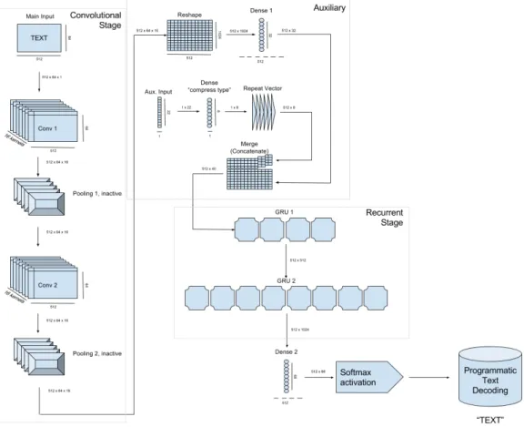
The deep net classifier is wholly implemented through layers natively present within the Keras deep learning library.The main 4 types of layers involved, which define the func-tionality of the classifier are called dense (also known as fully connected layer), merge, maximum pooling, 2d convolution and GRU. Besides these, the model also includes more or less auxiliary layers called input, reshape and repeat vector.The architecture is mostly intact from the original example implementation with the exception of the auxiliary input and changes in settings of the pooling layers.The classifier is more or less natively described as two distinct stages.Figure 3.1 provdies visual clue as to how are the stages interconnected.

. . . .

Figure 3.1. Figure depicting the overall structure of the OCkRE classifier

3.3.1

Convolutional stage

As explained by quite exhaustive explanation at deeplearning.net[15] , convolutional neural networks have strong justification as visual processing units with important par-allels to natural biological visual processing centres.Importantly, they maintain sparse connectivity or in other words, data passing through convolutional layers (or multiple) maintains the natural spatial “sense” it had before entering. They are very well suit-able for learning what basically serves as a replacement for both the “preprocessing” and “feature extraction” steps of the classic OCR as seen by Eikvil. Convolutional kernels can easily learn things like edge detection.This helps the classifier to deal with problems like variable degree of contrast between background and foreground. The convolutional layers implemented within OCkRE both maintain native input resolu-tion (512x64), operate each operating with 16 convoluresolu-tional kernels.They both use the Relu activation function, with border mode set assame. A convolutional layer we use represents a set of convolutional filters that each apply a fixed kernel at each point of input, as described in the following equation, as described by [16]

x`ij = m−<sub>X</sub> 1 a=0 m−<sub>X</sub> 1 b=0 ωaby`−_(i+1_a)(j+b).

Where we operate with some filterωover a two dimensional tensor to gain the input of some unitx. The convolutional classifier consists of two convolutional layers in a series, with a two dimensional maxpooling layer after either of the layers.As further elaborated on by the article on deeplearning.net[15], the pooling layers serve as a “smart” way of decreasing dimensionality of the passing through information.The convolutional stage

3. OCkRE OCR Implementation

. . . .

of the classifier has been left mostly intact as they have been set by the keras example source code with the exception of OCkRE effective disabling the pooling layers.This has been done by setting the pooling factor of both layers to 1, which has been done in effort to increase the practical visual accuracy and fine granularity of the visual data, allowed further down into the classifier, towards the recurrent stage.This however led to an increase in computational difficulty, but led to increase in the final accuracy of the classifier.

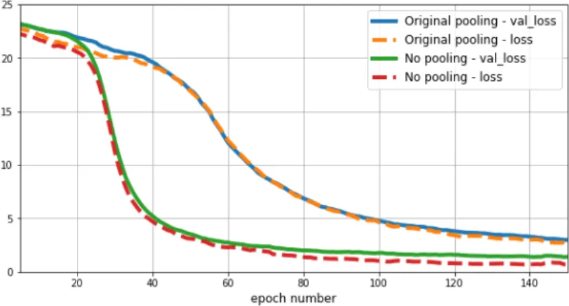
Figure 3.2. Comparison of behavior with and without pooling

This figure 3.2 of training log data illustrates advantage of classifier with pooling layers disabled. The lowest point of validation loss was 1.19 on the pooled classifier versus 1.07 on the one with pooling omitted.The training loss of the pooling classifier was at 0.31 at the best point while training loss of the unpooled classifier actually practically zeroed out.This experiment led to decision to disable pooling during further development of the classifier.

3.3.2

Recurrent stage

The recurrent stage of the classifier has been left mostly untouched by our effort and is as conceived by the author of the original keras example.The most crucial element of the later part of the classifier are the two successive bidirectionalGRU (Gated Recurrent Unit) layers. [Cho et al., 2014] As excellently explained and presented in Empirical Evaluation of Gated Recurrent Neural Networks on Sequence Modeling [17], GRU layers are similar to LSTM layers while omitting internal memory cells. The mathematical equations describing behaviour of GRU layers are as follows;

zt=σg(Wzxt+Uzht−1+bz)

rt=σg(Wrxt+Urht−1+br)

ht=zt◦ ht−1+ (1− zt)◦ σh(Whxt+Uh(rt◦ ht−1) +bh)

wherextis the input vector,htis the output vector,ztis the update gate vector and

rt is the reset gate vector, withW, U, bposing as the parameter matrices and vector.

As formulated per [17].

The greatest value of GRU and LSTM layers is their ability to maintain a short as well as a long term memory of the data sample being classified as it passes through the layer. In the case of our classifier, the data, as it comes from the convolutional stage. The width of the original image serves as the “time” axis, with individual columns of the post-convolution still image-like structure fed into the recurrent layers as a series.

. . . .

This sequence conscious capability is crucial for two reasons. Firstly, it allows for operation over variable length input in the sense that the text can be stretched over an arbitrary area of the input field, with various size and aspect ratio of individual letters, as well as varied in number of characters Secondly, it gives the classifier the capability to learn the quasi linguistic structures, without separate access to some dedicated model or dictionary to correlate the results of the classification with for purposes of error checking and error correction. In this sense, the recurrent stage of the network does all of the recognition and post processing and correction work steps expected as a separately engineered heuristic blocks of Eikvil’s era OCR. The GRU layers are set up with the following parametres:Their width is that of the native input width (512), they operate in thereturn sequences mode, the first operates in the mode which merges by summing, the other by concatenating.

3.3.3

Auxiliary structures

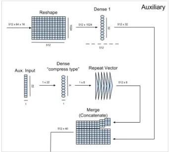
Between the convolutional and recurrent stage, there is several auxiliary layers. The output of the convolutional stage is cut down in dimensionality by a dense layer, with a necessary reshape happening on the entry into the dense layer as the Keras dense layer requires a flat entry vector, as opposed to the sixteen channels of raster like tensor grids coming from the convolution stack.In parallel to this, the auxiliary input carrying information about which type of a string is being processed goes through a dense layer of its own.The purpose of this dense layer is to allow the classifier to group the various types of strings it encounters based on shared qualities.For example, some of the currently recognised label types are “date due”, “date issue” and “date uzp”. While in the scope of the entire Morgan pipeline,the distinction between these types is crucial, for the OCkRE classifier, these all figure as structurally indistinguishable strings in common date formats. Similarly, the pipeline deals with many variants of “amount” data type, all of which are some monetary value. Again, the structural differences between individual types of “amount” are practically indistinguishable and irrelevant at the OCR level.With the dense layer present, the classifier can learn these groupings natively which also allows for better flexibility and scalability in the future as new format types are introduced.The output of the previously mentioned dense layers is concatenated together, forming a new series of heterogeneous “columns”;ones that contain a vector representing the visual data as processed by the convolutional stage with appendage of the “type” vector.These columns are passed on, into the recurrent stage of the classifier. Finally, the last layer in the classifier is another dense layer on the output of the recurrent stage which aids in transforming the output of it to the eventual character activations.

3. OCkRE OCR Implementation

. . . .

Figure 3.3. Figure depicting the structure of the auxiliary stage of the OCkRE classifier

3.3.4

Output of the deep classifier

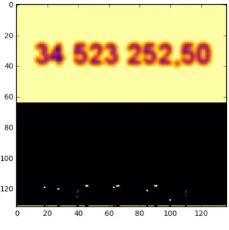
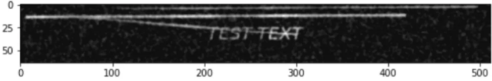
The final output of the classifier is in the form of a tensor with a width equal to the width of the input image and height equal to the number of character classes recognised plus one (the extra class figuring as “empty output”). A softmax activation function is applied to each column to select the prevailing column classification. The output string is decoded by grouping uninterrupted areas of activation and choosing the most prominent such a group, ignoring the blank label activations, except for distinguishing the transition to a new character..The nature of this output can be understood quite well from looking at a cropped out part of the output together with an input picture.

Figure 3.4. Output of a regular image

With a close look at Figure 3.4 one can recognise that individual pixel rows corre-spond with character classes. The digit 3 is represented by pixels on a row just under the one representing the digit 2, the digit 5 being yet lower than these, with the comma symbol being the lowest of them all.The sequence has been decoded as [’34523252,50’]

. . . .

if we forgive the missing space character, which had hints of activation, but the activa-tion wasn’t strong enough to beat the empty output symbol. The observaactiva-tion is ever more interesting when the same input is classified with some gaussian blur added.

Figure 3.5. Output of a blurred image

This input on Figure 3.5 has been decoded as [’34523252,60’],with the notable dif-ference being the error in the third digit 5 in the string, which has been decoded as a six, instead. One can easily see the amount of uncertainty of the classifier on what exactly are the third and second to last digits in the input.The activation is smudged into an indecisive column of possible options. In the first occurrence of digit five, it’s still decoded correctly, in the case of the last one, the decoding is incorrect.

3.4

Optimizer

A crucial element of machine learning is the optimizer. As stated in the work “Opti-mization Methods for Large-Scale Machine Learning”[18],the role of optimization in machine learning is to numerically compute parameters for a system designed to make decisions based on yet unseen data. It’s done so based on currently available (train-ing) data and choice of parameters that are optimal in respect to the given learning problem. A multitude of various algorithms can be used for solving this problem, Keras library implementing many of these options.The original keras example used the Keras implementation of SGD optimizer. Adam optimizer generally promises better results [19], so we have tried it experimentally, observing significant improvement especially in training time required.

3.4.1

SGD

Stochastic Gradient descent is currently somewhat of a baseline optimizer in machine learning. As explained by the deeplearning.net[20], what in principle distinguishes it from a regular gradient descent is that the calculation of gradient used for update in parametres of the classifier is based on just a subset (batch) of the training set samples, rather than the entirety of it, which allows the descent to proceed more quickly. Another advantage is that in practical implementations of the training apparatus as if for instance in Keras, updating with a training subset of some smaller size decreases

3. OCkRE OCR Implementation

. . . .

the maximal immediate working memory space required for calculating an epoch.The original Keras example set SGD with the parameters as follows; (lr=0.02, decay=1e-6, momentum=0.9, nesterov=True, clipnorm=5)

3.4.2

Adam

The core distinguishing feature of Adam as an optimizer is its estimation of adaptive learning rates for individual parameters in the system [19]. It is based on combining two earlier optimization methods, AdaGrad and RMSProp.In context of our work, the primary advantage of Adam is that by design, it’s more adaptive nature makes able to independently infer the optimal learning rate without need to experimentally look for the right parameters basic SGD would require.

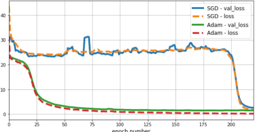
Figure 3.6. Comparison of behavior between the SGD and Adam optimizers

Figure 3.7. Comparison of behavior between the SGD and Adam optimizers focused on later moment in the training

These two figures compare loss as measured during training,one training using the original SGD optimizer, the other one using Adam.Each figure is focused on a different time period in the training. First graph shows that optimization driven by Adam converged to its optimum much faster than one driven by SGD, the second graph shows that even at its optimal point, SGD driven optimization actually came short of the minimal loss value achieved by the Adam optimizer. This experiment led to decision to use Adam optimizer in place of SGD. We have maintained default values for the Adam optimizer, as proposed by the original paper.

Chapter

4

Dataset structure implementation As explained by Alexander Wissner-Gross in his ar-ticle “Datasets Over Algorithms”[21], datasets can be an ever more important factor in machine learning than the design and implementation of the machine learner itself.The quality and quantity of training data has a critical effect on capability of the resulting classifier. Significant effort within our work went into design and implementation of a dataset structure to serve as means for extracting real world training data, fabricating synthetic training data and managing them in a format readily usable for training and evaluation. Once a supply of bot synthetic and real-world data samples has been es-tablished, training has been done on a random half-and-half mix of real and synthetic data, with the training data generator simply generating synthetic samples on the run, to mix in with the real world data. The performance of our classifier has only been regularly validated and tested on the real dataset, without contribution of synthetic data.

4.1

Dataset of the original Keras example

The original Keras example operated with a semi-synthetic dataset.It operated with a plain text dataset of real english words, distinguishing between monogram and bigram structures (single words and common pairings of words).These strings have been then used for synthesis of bitmap samples, utilizing the Cairo library for vector graphics [22] with the help of the cairocffi API for python [23].The text bitmaps produced by Cairo have been further augmented with speckle noise and deformations.

4.2

Real data extraction and handling in OCkRE

The codebase of this work responsible for extraction and handling of real world data strongly relies on the current inner functioning of the larger Morgan pipeline, and as such, is practically unusable outside of this broader code environment. For this reason, we sadly cannot include its code together with the rest released with this work. Furthermore, the real world training data itself comes wholly from a set of invoice documents, which have been confided to Rossum Ltd.with strict legal obligations that explicitly prohibit their further redistribution so none of it can be externally presented. In essence, the real world training data used for training of OCkRE has been obtained by programmatically extracting raster crop outs (from now on, “crops”) from raster scans of real world documents.The crops have been based on bounding boxes marked out on the documents by a team of labelers, each crop paired with a plain text “gold label” manually determined by the labeler. These labeled document serve as training data for many parts of the Morgan pipeline, including OCkRE. The whole real-world dataset obtained this way contained approximately 14000 unique crop outs. This set has been split to roughly 10000 crops intended for training and 4000 crops intended for evaluation. No further processing is performed on the extracted crops. During

4.

. . . .

training, the crops are inserted on pseudo-random position within the 512x64 pixel input bitmap, with pseudo-random variation in scale. During evaluation and testing, crops are always padded to the center of the input raster, without changing the scale, their native resolution being maintained.

4.3

Synthetic data generation

Obtaining a sizeable and representative enough dataset is often one of the biggest chal-lenges in machine learning tasks. While we could operate with the aforementioned corpus of 14000 “crops” more or less from the beginning of development, it quickly became apparent that the classifier begins overfitting on the training data.To remedy this, there has been significant effort made into implementing a synthetic sample gen-erator that would well supplement the real data.In training the OCkRE, we mix real and synthetic data 1:1 and evaluate only on real data. The software submitted along with this thesis relies solely on the synthetic data for both training and evaluation.The synthetic data generation can be divided into two stages.

4.3.1

Strings

The first step in generating relevant synthetic training data is ensuring the information encoded within the text is sufficiently similar to the real world strings we can expect to be eventually classifying. While this isn’t particularly important for the convolutional stage of the network which focuses on the visualqualities of the data, it is absolutely crucial for the recurrent stage. It allows the recurrent stage to learn the typical infor-mation structures, for instance the syntactic format of dates with commas separating the number of day from the number of month and number of year. For this reason, the author of the work has proposed a set of functions that generate quasi random information, following the structural rules that attempt to mimic those found in the real world data. The initial implementation of these functions has been done by our colleague Světlana Smrčková and afterwards refined and completed by us. This gen-erator of synthetic strings is implemented as a separate module to be called from the context of the dataset handling structures.

4.3.2

Text bitmaps

The second step in generating synthetic training data is rendering the strings from the previous step as a bitmap. OCkRE bases its rendering pipeline on the one already present in the original Keras example, modifying it and further expanding its function-ing. The text is still rendered using the Cairo vector graphics library as in the original, and the “speckle” noise augmentation is still utilized, however the original library’s “skewing” which deformed the text unevenly has been discarded as not a good repre-sentation of distortion seen in our real world scenarios.Further steps of augmentation have been implemented in effort to mimic the usual imperfections as seen in real world text scans. Compared to the original implementation, OCkRE underwent an effort to include more font families and shapes, compared to the set used in the original example. OCkRE also implemented pseud-random variance in size of the text used, rather than maintaining a stable size.

4.4

Visual augmentations

OCkRE utilizes a series of visual augmentations meant primarily to make the training data similar to real world cases, degrading the visuals to increase the difficulty of the

. . . .

task and prevent overfitting.In this sense, the term “augmentation” might be somewhat confusing, as the data samples become harder to read accurately, for classifiers as well as any human operator.It’s however the value of the sample as something that allows the classifier to learn more general classification capability of it that is getting augmented, even though the samples visually appear “uglier”. The only decisive metric for how severe can the augmentation be to still count as passable is a very practical one - as long as a human can read the text, the augmentation is acceptable.Now, in the massive volume of samples used during training, this condition might not always be fulfilled, however this is considered to be an acceptable shortcoming of the design.The individual augmentation steps in the OCkRE do get selected in pseudo-random way, for instance with some degree of blur being applied to almost all synthetic samples, however for example full contrast inversion is kept relatively rare.Multiple augmentations can also be applied to a single sample as a series. These rules are set on basis of our rough subjective observations of quality of real world samples, to if possible be relatively similar to them.

4.4.1

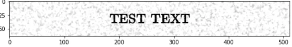
Speckle

“Speckle” noise has been adopted from the original example. It is implemented as granular noise made smoother through gaussian blurring of pseudorandom intensity. OCkRE decreases the maximal amount of blur applied to the noise mask at this point, as the newly implemented separate blur augmentation step tended to blur the text too much. Functionally, speckle is implemented through addition of a numpy matrix with the aforementioned qualities, to the raster, after the text has been rendered. Speckle augmentation allows the classifier to gain some robustness against the commonly present visual noise on scans caused by visible particulate in lower quality paper, various surface impurities on the scanned pages, as well as flaws in optics of the scanner.

Figure 4.1. Example of the speckle augmentation

4.4.2

Line noise

OCkRE implements another kind of pseudo-random noise compounded into the image similarly to speckle, however this noise having the form of randomly positioned straight lines of varied thickness. Line noise is implemented as a function step using the Cairo library while the prepared synthetic sample is still represented within vector space of Cairo. This allows for easily implemented semi-transparent lines which can be of a different contrast level than the text (for instance, gray lines around black text) and cross over text, without actually disturbing geometry of the characters and visually appearing as to be “behind” the text. It also ensures easy application of anti-aliasing on the lines. Earlier attempts at implementing line noise as a separate, later step on the raster level lacked these qualities. These lines are a very naive approach at simulating the commonly appearing remainders of formating tables which sometimes end up included into the crop due to inaccuracy of the area marked as the space the text occupies. Inaccuracy in area definition has to be expected even in production environment during classification, so it is crucial for the classifier to learn to ideally ignore this kind of noise.

4.

. . . .

Figure 4.2. Example of the line noise augmentation

4.4.3

Blur

The simplest augmentation utilized is basic gaussian blur. While lack of visual focus isn’t a common issue among scanning devices, OCkRE might eventually be expected to recognise characters as photographed with an all purpose photographic camera, where lack of focus is a common issue.At the same time, gaussian blur causes effects somewhat reminiscent of the source text being smudged or fuzzed by presence of a liquid or mechanical friction.

Figure 4.3. Example of the blur augmentation

4.4.4

Clouding

OCkRE implements clouding in attempt to simulate localised smooth variations in contrast that seem to be another common imperfection in regular scanned documents. We aren’t completely certain what causes this imperfection in reality. It might be uneven adhesion of laser printer toner, lost pigment due to mechanical handling or some other such damage. In practice, it makes some areas of the text lower contrast than others, however without necessarily blurring the edges of the text.Within OCkRE, it is implemented somewhat similarly to speckle noise.A raster mask is covered in pseudo-random rectangles, which are then heavily blurred via gaussian blur to the point of reminiscing of “clouds”. This mask is then applied additively to the raster with the original text, brightening some areas of the text.It’s crucial that this step is performed before introduction of speckle noise or other background-wide changes as it’s intended to only influence the text itself (and potentially the synthetic “line” noise too,as the real world tables which it’s meant to simulate are subject to this phenomena as well) without changes to the background.

Figure 4.4. Example of the clouding augmentation

4.4.5

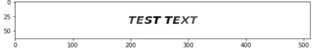
Contrast and inversions

The contrast manipulation augmentation doesn’t attempt to replicate any kind of un-wanted visual deterioration but simply mimic the phenomenon of some text being naturally printed with other than black-on-white contrast.In general case, some nat-urally occurring text is outright inverted in contrast - the text is brighter than the

. . . .

background. The contrast augmentation pseudo-randomly modifies the contrast level between the text and the background, simulating lower level contrast (light gray text on dark gray background) as well as the aforementioned inverted scenario, however attempts to ensure there is always sufficient amount of contrast left.

Figure 4.5. Example of the variable contrast augmentation

Figure 4.6. Example of the contrast inversion case of the contrast augmentation

4.4.6

Compounding

All in all, when multiple augmentation functions compound in a series, the results are quite noisy and varied.

Figure 4.7. Example of interplay between multiple augmentations

Figure 4.8. Example of interplay between multiple augmentations

Chapter

5

Means of evaluation

5.0.1

CTC Loss

OCkRE maintains the use of CTC loss metric as originally implemented by the Keras example. The CTC Loss, as defined by the paper “Connectionist Temporal Classifi-cation: Labelling Unsegmented Sequence Data with Recurrent Neural Networks”[24] allows effective calculation of the loss function in the precarious case with unsegmented input data which contains the desired information spread over a region of unknown position and unknown length (position of the text is random, scale of characters is varied). CTC loss, as presented by the aforementioned work manages all this without any additional information needed on nature or structure of the entry data.

5.0.2

Mean Normalized Edit Distance

A very convenient and human way of measuring accuracy of some processed text is Mean (Normalized) Edit Distance. OCkRE keeps this functionality intact from the original Keras example, utilizing external python package editdistance [25] which simply calculates it for any two strings provided based on algorithm as proposed by Heikki Hyyrö [26]. Mean Edit Distance describes the number of character edits required to get from one one string to the other one. Mean Normalized Edit Distance accounts accounts for the length of the strings compared, but as elaborated by Heikki Hyyrö, cannot be calculated simply by dividing the number of necessary edits by the length of the strings.

5.0.3

Label Accuracy

Another relevant metric, which might be seemingly redundant to MNED, is label-wise accuracy. Unlike MNED, it only distinguishes if two strings are actually equal, or not. The important detail is, that with a per-character error rate of just one wrongly classified character out of ten, in the edge case where all classified strings are exactly ten characters long and each has just one error, this can mean not a single one of the strings ends up classified correctly, so while mean normalised edit distance is just 0.1, one out of ten, the resulting accuracy over labels would be 0Particularly in a system where we attempt to extract exact information like bank account numbers and business ID numbers, a single character error already makes the information worthless.This makes Label Accuracy the more serious, crucial metric.

Chapter

6

Evaluation of achieved performance

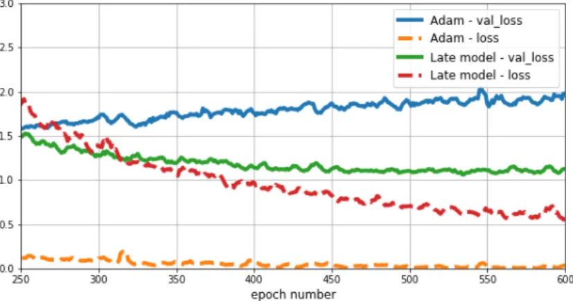
The final version of the synthetic data augmentations described within our work signif-icantly increased difficulty of training.So much is apparent from the following graphs comparing one of the last performed training runs to the run done much earlier to evaluate performance of Adam, which has been already shown once earlier in this work, to compare performance with the SGD optimizer. The “late model” still uses Adam optimizer as well, however, the Adam model did not include inference based on label type, and used simpler, unrefined and easier augmentation stages than the “late model” which was trained with full power augmentations as presented earlier in this paper.

Figure 6.1. Comparison of behavior between early and final model

Figure 6.2. Comparison within the same run but at later time

6.0.1

Performance in comparison with Tesseract

The final practical accuracy over whole strings of OCkRE on the validation (real world) dataset was measured at 92.13%, calculated as success rate with the criterion being string match with the exception of blank space characters which have been ignored. Tesseract OCR’s classification on the same dataset, measured by the same criterion achieved accuracy of only 77.02%.

Chapter

7

Conclusion

We have familiarized ourselves with functioning of the Keras OCR example as well as broader functioning of the Keras library and many overreaching machine learning concepts, techniques and principles. Utilizing an existing implementation of an OCR example originating from the Keras project library capable of classifying short strings as a starting point, we have broadened its capabilities to function with longer strings, extended the set of characters it is capable of recognizing. We have adapted and extended augmentation for a noisier input and observed improvements in our use case. We have evaluated final performance of OCkRE and noted a considerable accuracy improvement in comparison to the previously utilized solution (Tesseract OCR) on our real world validation data set.This performance increase has been however achieved at cost of specialising on set of arbitrary strings - OCkRE would be likely rather impractical as a general OCR intended for reading of regular language based text. This however hasn’t ever been it’s intended purpose.

Appendix

A

Attached files

The DVD medium attached to this work contains following files; synthset.py, fakestrings.py, quicktest.py, traintest.py, ockre.py, OCkRE.pdf (a virtual copy of this document), densified labeltype best.h5, README, LICENSE keras

References

[1] ABBYY. What is OCR and OCR Technology. 2017.

https://www.abbyy.com/en-ee/finereader/what-is-ocr/.

[2] Adnan Ul-Hasan. Generic Text Recognition using Long Short-Term Memory Net-works. Ph.D. Thesis, 2016.

http://nbn-resolving.de/urn/resolver.pl?urn:nbn:de:hbz:386-kluedo-43535.

[3] Adnan Ul-Hasan, and Thomas M. Breuel. Can We Build Language-independent OCR Using LSTM Networks?. In: Proceedings of the 4th InternationalWorkshop on Multilingual OCR. New York, NY, USA: ACM, 2013. 9:1–9:5. ISBN 978-1-4503-2114-3.

http://doi.acm.org/10.1145/2505377.2505394.

[4] Line Eikvil. OCR - OpticalCharacter Recognition. 1993. [5] Scancorporation LLC. OCR Data Entry Products.

http://scancorporation.com/ocrproducts.html.

[6] L.P. Hewlett-Packard Development Company. OCR: The most important scanning feature you never knew you needed.

http://h71036.www7.hp.com/hho/cache/608037-0-0-39-121.html.

[7] Ubuntu Documentation - Holger Gehrke. OCR - OpticalCharacter Recognition.

https://help.ubuntu.com/community/OCR.

[8] Ray Smith. An Overview of the Tesseract OCR Engine. In: Proc. Ninth Int. Con-ference on Document Analysis and Recognition (ICDAR). 2007. 629–633.

[9] Google Inc. Ray Smith. Building a MultilingualOCR Engine.

https://github.com/tesseract-ocr/docs/blob/master/das_tutorial2016/7Building%20a%20Multi-Lingual%20OCR%20Engine.pdf.

[10] Tesseract github Wiki. 4.0 with LSTM .

https://github.com/tesseract-ocr/tesseract/wiki/4.0-with-LSTM. [11] Tesseract github Wiki. Home.

https://github.com/tesseract-ocr/tesseract/wiki. [12] Mike Henry. Keras OCR Example.

https://github.com/fchollet/keras/blob/master/examples/image_ocr.py. [13] Tensorflow home page. About TensorFlow.

https://www.tensorflow.org/.

[14] Theano home page. About TensorFlow.

http://www.deeplearning.net/software/theano/.

[15] Theano Development Team. ConvolutionalNeural Networks (LeNet).

http://deeplearning.net/tutorial/lenet.html. [16] Andrew Gibiansky. ConvolutionalNeural Networks.

http: / / andrew . gibiansky . com / blog / machine-learning / convolutional-neural-networks/.

. . . .

[17] Junyoung Chung, Çaglar Gülçehre, KyungHyun Cho, and Yoshua Bengio. Empiri-cal Evaluation of Gated Recurrent Neural Networks on Sequence Modeling. CoRR. 2014, abs/1412.3555

[18] Nocedal Jorge Bottou Léon, Curtis Frank E. Optimization Methods for Large-Scale Machine Learning. ARXIV. 06/2016, eprint arXiv:1606.04838

[19] Diederik P. Kingma, and Jimmy Ba. Adam: A Method for Stochastic Optimization. CoRR. 2014, abs/1412.6980

[20] Theano Development Team. Stochastic Gradient Descent.

http://deeplearning.net/tutorial/gettingstarted.html#stochastic-gradient-descent.

[21] Alexander Wissner-Gross. Datasets Over Algorithms.

http://deeplearning.net/tutorial/gettingstarted.html#stochastic-gradient-descent.

[22] Cairo team. Cairo homepage. 2014.

https://www.cairographics.org/. [23] Simon Sapin. Cairocffi github. 2016.

https://github.com/Kozea/cairocffi.

[24] Alex Graves, Santiago Fernández, and Faustino Gomez. Connectionist temporal classification: Labelling unsegmented sequence data with recurrent neural networks. In: In Proceedings of the International Conference on Machine Learning, ICML 2006. 2006. 369–376.

[25] Hiroyuki Tanaka. editdistance gitlab. 2016.

ttps://www.github.com/aflc/editdistance.

[26] Heikki Hyyrö. Explaining and Extending the Bit-parallel Approximate String Matching Algorithm of Myers. .