Fast Edge-preserving Gravity-like Image Interpolation

Fast Edge-preserving Gravity-like Image Interpolation

Željko Lukač1,3_{, Stanislav Očovaj}1,3_{, Dragan Samardžija}2,3_{, and Miodrag Temerinac}3

1 _{RT-RK Institute for Computer Based Systems,}

Narodnog Fronta 23a 21000 Novi Sad, Serbia

{ zeljko.lukac, stanislav.ocovaj }@ rt-rk.uns.ac.rs

2 _{Nokia Bell Labs, 101 Crawfords Corner Road,}

Holmdel, New Jersey, USA [email protected]

3 _{University of Novi Sad, Faculty of Technical Sciences,}

Trg Dositejа Obradovicа 6, 21000 Novi Sad, Serbia [email protected]

Abstract. In this paper we propose a novel image interpolation algorithm which preserves edges and keeps a natural texture of interpolated images. The algorithm is based on an idea that only pixels that belong to the same side of an edge should be used in interpolation of pixels that belong to an edge. Beside similarity-based separation of known interpolation pixels a gravity-like interpolation coefficient set is also introduced in order to support different number of interpolation pixels and their location in two dimensional plane. The algorithm also applies arbitrary scaling factors, thus offering a broader scope of applications. Use of a local set of interpolating points makes the proposed algorithm suitable for applications on resource-limited platforms. The edge performance is demonstrated for structured geometric forms, while a general interpolated image quality is evaluated using objective measures and subjective comparisons. A comparison with some relevant interpolation algorithms shows the desirable tradeoff between image quality (sharpness and texture) and requested computing power (run-time).

Keywords: edge directed interpolation, edge preservation, image interpolation, image processing.

1.

Introduction

In many applications, there is a mismatch between the original and desired image resolution. For example, multimedia systems are facing the problem of how images in many different formats can be presented on displays with different resolutions. Furthermore, in medical and satellite image diagnosis and analysis, an enhanced resolution is preferred. In order to provide improved resolution, image interpolation techniques are applied.

at the pixels of the original image. Considering the interpolation problem in the spectral domain, changing the sampling frequency redefines the spectrum range and missing spectral components cannot be reconstructed from the known spectrum of the original image. This problem does not have a unique solution. Therefore, there are many proposed algorithms considering specific frame conditions in different applications. The main problem in image interpolation is to preserve the natural appearance of image texture while maintaining edges, i.e., the image sharpness. These are two mutually opposing requirements and most of interpolation algorithms pursue one of them better than the other. Furthermore, in many applications, an arbitrary scaling factor (not only integer) is requested.

The other aspect of image interpolation is complexity of used algorithms. For certain applications almost unlimited computational resources are available, however, for most of them a compromise between interpolation complexity and expected quality must be made.

In this paper we propose a novel image interpolation algorithm. The proposed algorithm is based on two original contributions: (i) similarity grouping of interpolating pixels (preserving image sharpness) and (ii) gravity-like interpolation (providing natural appearance of texture). The original pixels are grouped according to their similarity and then a new interpolated pixel is generated using the group it is affiliated with. The gravity-like interpolation coefficients are proportional to the inverse of the square distance between an interpolated pixel and known interpolating pixels. Unlike some other well-known solutions, the gravity-like interpolation applies arbitrary scaling factors. In Section II, the problem identification and related work are presented. In Section III, the proposed algorithm is described. Basic properties of this scheme are evaluated in Section IV. In Section V, the proposed solution is compared against five referenced interpolation algorithms using four the standard image quality measures: the structured similarity index measure (SSIM) [33], the sharpness measure (SM) [13], the peak signal to noise ratio (PSNR) [32], and blind image quality index (BIQI) [23]. Finally, Section VI concludes the paper.

2.

Problem identification and related work

2.1. Problem identification

An interpolation algorithm is applied to an original image with { Iin(v, h, c); v = 1,…, V ,

h = 1,…, H and c = 1,…, C } where V and H are the number of pixels in the vertical and horizontal dimension and C is the number of color components (C = 1 for grey images and C = 3 for color images). For a given scaling factor F, the interpolated image pixels are { Iout(p, q, c); p = 1,…, Vout and q = 1,…, Hout , c = 1,..,C } where vertical and horizontal image sizes are Vout = F

.

V and Hout = F .

h F q h v F p v F q h F p v c h v I c h v I c h v I c h v I in in in in                _       _            1 1 1 1 1 1 1 1 ) , 1 , ( ) , , ( ) , 1 , 1 ( ) , , 1 (

(1)

where v and h are the remainder coordinates (vertical and horizontal) in the rectangle defined by the above pixels.

Fig. 1 (a) rasters of original and interpolated images and (b) four-point neighborhood by the scaling factor F = 1.5

2.2. Related work

In this paper, we are addressing applications with limited resources where a tradeoff between image quality (texture and edge quality) and requested computing power (run-time) should be analyzed. Considering these two aspects (texture vs. sharpness and complexity vs. expectations) image interpolation algorithms can be categorized in the following groups. The first group consists of the least complex algorithms, such as sample and hold (SH) [12], bilinear (BL) [12] and bicubic (BC) [17], with limited image quality. The second group includes low-complexity algorithms that preserve edges (image sharpness). This approach has been originally demonstrated in [3] and improved in recently published algorithms: adaptive image scaling based on local edge directions (LAI) [18], image magnification using interval information (KI) [16] and fast image interpolation using directional inverse distance weighting for real-time applications [15]. The third group of algorithms such as [10], [11], [19], [20], [28], [30], and super-resolution convolutional neural network (SRCNN) [8] are characterized by complex image analysis, increased complexity and good interpolation results.

Additionally, the arbitrary scaling factor is provided by algorithms SH [12], BL [12], BC [17], and LAI [18]. In contrast, the algorithms [3], KI [16], [10], [11], [19], [20], [28], [30], and [15] allow only integer scaling factors. For the algorithm SRCNN [8] model parameters have been provided for integer scaling factors only.

v h

Iin(v+1, h) I_in(v+1, h+1)

I_in(v, h) I_in(v, h+1)

Representatives from all three algorithm groups will be further examined in this study. Namely, the SH and the BC algorithms from the first group, the LAI and the KI algorithms from the second group and the SRCNN algorithm from the third group will be used for image interpolation performance analysis. The regularized local linear regression (RLLR) [20] and adaptive sparse domain selection (ASDS) [10] will be used in complexity analysis.

Design of interpolation algorithms is a trade-off between computational complexity and image quality. Algorithms based on an a priori knowledge about whole image provide better image quality but require higher computational complexity. Algorithms based on an a priori knowledge in a closer neighborhood of interpolated pixel decrease computational complexity but also decrease image quality. Image quality is defined by structural quality (preservation of edges) and natural outlook (texture) of an interpolated image. Therefore, the design of interpolation algorithms always faces three significant decisions:

• The size of processed neighborhood around an interpolated pixel having a direct impact on computational complexity and image quality (the smallest processing size is 2x2 neighboring pixels of the original image);

• Preservation of edges for identified image structures; and

• Interpolation rule (calculating of an unknown image value at an interpolated pixel from known values at neighboring pixels of original image) guarantying a natural image outlook (texture).

3.

Similarity grouping interpolation algorithm

3.1. Sorting of image values

The four pixels of the original image (1) are grouped in two regions according to similarity of their values. The process starts with a sorting of values of interpolation pixels. Interpolation pixels are ordered in the two dimensional array and prior to the sorting they need to be ordered in the one dimensional array (2D to 1D ordering is defined in (2)). The four pixels from two dimensional array Iin are ordered in a sequential array S, separately for each color component (c):



2(v_s1)h_s,c



I_in(vv_s1,hh_s1,c) v_s 1,2 h_s 1,2.

S (2)

The four indices of this array correspond row-wise to the indices of the

four interpolation pixels:













2

1

4

3

.

The sequential array S is sorted according to its values (the smallest first) what also defines the four indices (nc) of the sorted array from the original set [1,2,3,4]:







(1),

 

(2),

 

(3),

 

(4),



. as such ) ( 4 ,..., 1 ), ( ) ( c n S c n S c n S c n S k n k c k n S k S c c c c c c c     

(3)

3.2. Similarity grouping

After values of interpolation pixels are sorted they need to be grouped according to their similarity. This is done by finding the maximum difference between values of neighboring interpolation pixels in the sorted array.

The maximum difference Dc,max between neighbors in this sorted array |Sc(k, c) -

Sc(k+1, c)| is determined (k = 1, …, 3), together with its position kc,max (1, 2 or 3). Then, the color component c* with the maximum image value difference Dc*,max defines the splitting index kc*,max and the list of original indices nc*,(k). The list nc*,(k) and splitting index kc*,max are used to form two groups of image pixels with the corresponding lists of original indices n1 and n2 such as









. 4 ,..., 1 ) ( ) ( ,..., 1 ) ( ) ( , max arg * , max : , max *, max *, * 2 max *, * 1 ,..., 1 max , ,..., 1 max , max *, * max *, c c c c c C c c C c c c c c k k k k n k n k k k n k n D c D D n k          

(4)

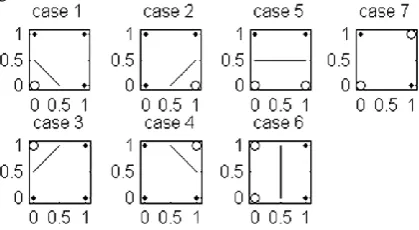
Two kinds of pixel partitions in two groups are possible: 1:3 (kc*,max = 1 or 3) or 2:2 (kc*,max = 2). The third possibility (0:4) is allowed if the maximum difference Dc*,max is smaller than a predefined threshold Dth (kc*,max = 0). In total, there are seven possible cases of how the original pixels are partitioned.

Setting the threshold to low value is not that critical since it is used in edge detection in conjunction with other criteria. Experimental results presented in this paper are obtained with Dth value set to 10.

3.3. Affiliation of the interpolated pixel

Interpolation pixels are divided into two partitions according to their similarity in the previous step. Before a new pixel is interpolated, it has to be affiliated with a particular partition. The original pixels in the selected partition will be used for interpolation. Seven different partition cases are depicted in Fig. 2, where cases 1 to 4 correspond to the 1:3 partitioning (corner edges), cases 5 to 6 correspond to the 2:2 partitioning (horizontal and vertical edges), and case 7 corresponds to the 0:4 partitioning (no edges).

A decision on which case is actual is based on the pattern recognition of the sorted image order:



 





 





 







 







 







 







 









 







                                      ] 3 , 2 [ ] 4 , 1 [ 2 7 4 , 2 [ ] 3 , 1 [ 2 6 4 , 3 [ ] 2 , 1 [ 2 5 3 ) 1 ( 1 ) 1 ( 1 1 max , max , 1 1 max , max , 1 1 max , max , max , max , 2 max , max , 1 * * * * * * * * * * n n k D D n n k D D n n k D D k D D n k D D n case c th c c th c c th c c th c c th c

(5)

For each case in Fig. 2, the lines represent the assumed linear edge orientation. However, for case 7 the edge orientation is unknown, therefore it is also considered as the 0:4 partitioning.

Fig. 2. Seven possible cases of partitioning with lines corresponding to the assumed edge orientation (cases 1-4 diagonal edge, case 5 horizontal edge, case 6 vertical edge, and case 7 no edge).



1,2,3,4



: 7 ], 4 , 2 [ 5 . 0 ], 3 , 1 [ : 6 ], 4 , 3 [ 5 . 0 ], 2 , 1 [ : 5 ], 3 , 2 , 1 [ 5 . 1 ], 4 [ : 4 ], 4 , 2 , 1 [ 5 . 0 ], 3 [ : 3 ], 4 , 3 , 1 [ 5 . 0 ], 2 [ : 2 ], 4 , 3 , 2 [ 5 . 0 ], 1 [ : 1 2 2 1 2 1 2 1 2 1 2 1 2 1                                                                  n n case otherwise n h n n case otherwise n v n n case otherwise n h v n n case otherwise n h v n n case otherwise n h v n n case otherwise n h v n n case i i i i i i i

(6)

where ni is the list of pixel indices belonging to the selected partition, v and h are the remainder coordinates defined in (1). For example, in case 1, if the new pixel is above the line, the original pixels 2, 3 and 4 will be used for interpolation.

3.4. Gravity-like interpolation

The interpolated pixel value is generated using the original pixels defined by the interpolation index list:



 

i



i i

L

k i

out pqc wn k S n k c L length of n

I i   



 ), ( ) ( ) , , ( 1

(7)

where w(ni(k)) are the interpolation coefficients. Note that L can take any value from 1 to 4 (i.e., for L = 3 interpolating pixels define triangle and interpolated pixel is in its interior). Therefore, use of conventional interpolation algorithms is not always possible.

The novel interpolation algorithm called gravity-like interpolation is based on the analogy to the gravity law:





i

i

i k L

k n d Q k n

w 1,...,

)) ( ( )

(  ₂  (8)

where d(ni(k)) are the squared Euclidean distances of the four adjacent pixels to the interpolated pixel: . 2 , 1 2 , 1 ) 1 ( ) 1 ( ) 2 ) 1

(( 2 2

2              h v v v h h h v

d (9)

The condition for zero gain interpolation (the output range should be the same as the input range) is given by:

. 1 )) ( ( 1 



 i L k i k n

w (10)

. ,..., 1 )) ( (

)) ( (

)) ( (

1 1

2 1

2

i L

r L

r m m

i L

k m m

i

i k L

m n d

m n d

k n w

i i i

 

 



    

(11)

For example, in the case of one interpolating pixel (Li = 1) there is only one interpolation coefficient with value one, which corresponds to the SH interpolation.

4.

Evaluation of basic properties

Two basic properties significant for quality of interpolation are analyzed and compared with other interpolation algorithms: edge preservation and edge integrity.

4.1. Edge preservation

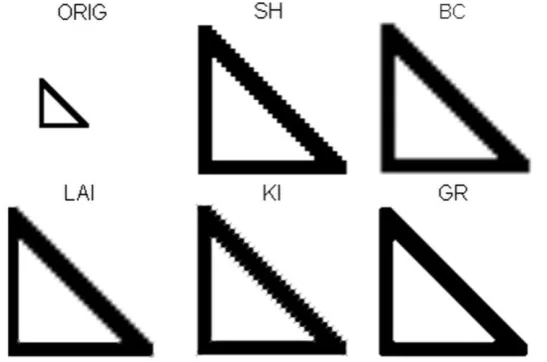
Advantage of the proposed algorithm in edge preservation is shown in Fig. 3 using a simple black and white image of a triangle with typical three edge directions: horizontal, vertical and diagonal. The analyzed interpolation algorithms can be used to magnify (F

> 1) or reduce the image size (F < 1). Since more illustrative, image magnification is considered.

Fig. 3. Image interpolation results for F = 3: a) original image, b) SH, c) BC, d) LAI, e) KI, f) GR.

horizontal edges but introduces certain artifacts on the corners and diagonal edge. The proposed GR algorithm preserves all edges well. However, it slightly rounds the corners.

4.2. Edge integrity

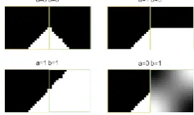
An inherent property of the proposed interpolation solution is the edge integrity preservation – no discontinuities of edges between the two interpolation rectangles corresponding to neighboring interpolated pixels. This property is easy to illustrate with an example of binary images (value 0-black and 1-white). The example is given for the right-vertical side of the interpolation rectangle. Assume a four-pixel constellations for two neighboring interpolated pixels of the original image and next to it on the right-hand side there are four possible constellation combinations: (a, b) = {0, 1} as shown in Fig. 4.

Fig. 4. An example of interpolation rectangle (dashed) and adjacent interpolation rectangle (dotted). Two right most pixels of adjacent interpolation rectangles have values a and b.

For all four cases, the results of interpolation are shown in Fig. 5 illustrating the edge integrity preservation.

Fig. 5. An illustration of the edge integrity preservation in an example for a scaling factor F = 20

4.3. Gravitation like interpolation

We did not find any previously-published ideas similar to our proposal how to generate interpolation coefficients using analogy with the law of gravitation:

Iin(v+1, h) I_in(v+1, h+1)

I

in(v, h) Iin(v, h+1)

I_in(v+1, h+2)







    













_L

p L

p m m

k L

k m m

k

k k L

k

k in k k

out

c

I

c

I

1 1

2 1

2

1

)

,

(

)

(

)

,

(

)

(

x

x

x

x

x

x

x

x

x

x

(12)

where Iout(x) is the value of the interpolated pixel and Iin(xk) are known interpolation pixels defined by the coordinates x and xk, respectively. In general, x and xk can be N -dimensional vectors in N-dimensional space. Thus, the algorithm application is not limited to 1 or 2 dimensions.

Besides the main advantages of this approach: applicable for any number of interpolating points, better edge-preservation and guaranteeing integrity of edges, more detailed evaluation of this approach also shows some additional advantages.

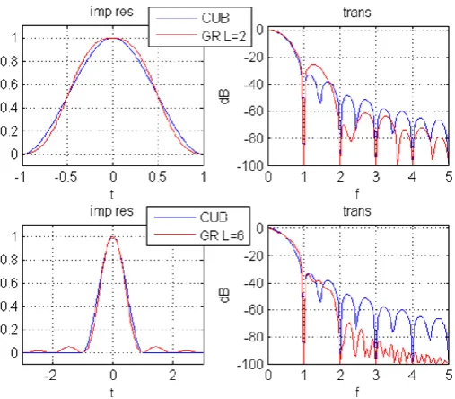
An illustration of those features for the gravity-like interpolation could be seen in a simple 1D example. The 1D impulse responses with the corresponding transfer functions (anti-aliasing LF filters) are shown in Fig. 6 for the cubic (CUB) and gravity-like (GR) interpolation using two lengths L = 2 and L = 6.

Fig. 6. Impulse responses and amplitude transfer functions for 1D cubic and gravity-like interpolation

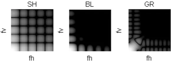
The 2D impulse responses with the corresponding transfer functions (anti-aliasing LF filters) are shown in Fig. 7 for the SH, the BL and the GR interpolation algorithms. These two simple algorithms are used to emphasize the main advantages of the new algorithm. It is assumed that for the GR algorithm all four pixels are used (Li = 4), same as in the SH and BL interpolation.

Fig. 7. Impulse responses of interpolation filters for SH, BL and GR interpolation; scaling factor

F = 20 and response size 40 x 40 pixels.

The SH impulse response is a rectangle around the impulse pixel. The BL impulse response has a circular shape but with pronounced vertical and horizontal directions. The impulse response of the proposed gravity-like interpolation (GR) has a circular shape with uniform values in all directions.

The transfer function of the interpolation filter is the Fourier transform of the impulse response. Theoretically, it should be a low-pass filter in both directions with a cut-off frequency of 0.5/F, where F is the scaling factor. In this case all possible aliasing components at higher frequencies would be suppressed, however the edges would be also blurred. Transfer functions of the three evaluated interpolation methods are shown in Fig 8.

Fig. 8. Amplitude transfer functions (white 1: 0 dB and black 0: below -60 dB) of interpolation filters for SH, BL and GR interpolations; frequency ranges in both directions (fv and fh) are

between 0 and 0.25 (normalized).

quality is better, however edges are blurred. Likewise, the GR transfer function suppresses high-frequency components. Nevertheless, it results in uniformly distributed artifacts, thus leading to improved perceptual image quality.

5.

Comparison with other interpolation algorithms

The proposed solution will be further compared with other five widely known interpolation algorithms: SH, BC, LAI, KI and SRCNN. The following comparisons are considered: objective quality measures and subjective quality impression.

5.1. Reference test database (LIVE)

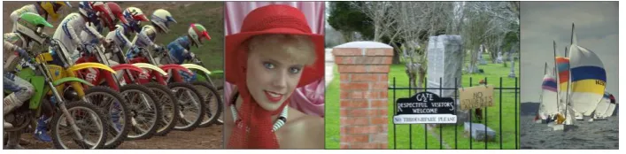
Experiments were performed on all 29 reference images from the reference test database named LIVE [25]. The test database LIVE is widely used in evaluation of quality of various image processing algorithms. Some considered (typical) images from this database are shown in Fig 9. The image Bikes is a represent of complex images. The image Womanhat represents portrait images. The image Cemetry contains letters and the image Sailing2 represents images with large homogeneous areas.

Fig. 9. Examples of typical images from the test database LIVE.

5.2. Objective comparison

interpolation quality of texture and edges, respectively. Additionally, the traditional PSNR measure (the simple mean square error between original and interpolated images) has been also considered having in mind its disadvantages [32].

The original images were converted to 8 bit grayscale. The mean values of three measurements (PSNR, SSIM and SM) for all 29 reference images from the LIVE database are calculated for different scaling factors applying considered interpolation algorithms. For the KI algorithm, the results are shown only for integer scaling factors (non-integer scaling factors are not supported). That is also the case for the SRCNN algorithm, for which only model parameters used for scaling by factors 2, 3 and 4 are provided. For other algorithms, the results for non-integer scaling factors are also presented.

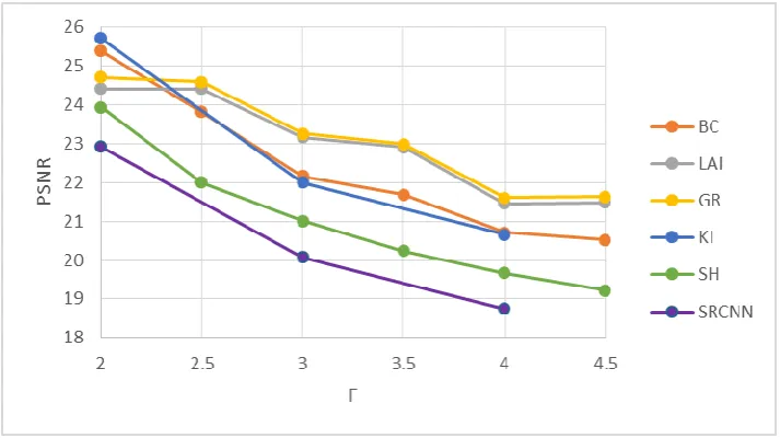
The evaluation results based on the traditional PSNR measure are shown in Fig. 10. The proposed method shows the best result for all scaling factors but 2, where BC and KI show slightly better result.

Fig. 10. The PSNR measure for different scaling factors – average for 29 LIVE reference images

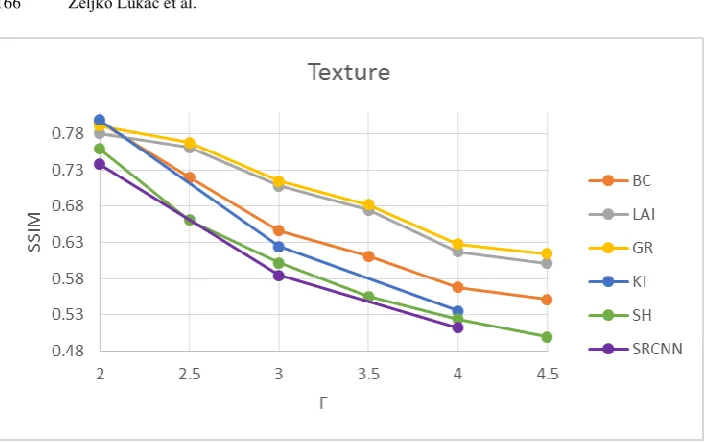
Fig. 11. The SSIM measure for different scaling factors – average for 29 LIVE reference images

For evaluation of edge preservation property the SM measure is used and results are shown in Fig. 12. The proposed method shows the better results for almost all scaling factors. However, for the scaling factor 2.5 the SH method performs slightly better as well as for the scaling factor 4 where the KI method is better.

Fig. 12. The SM measure for different scaling factors – average for 29 LIVE reference images

proposed in [22]. The given results correspond to averaged measures values for all 29 reference images for scaling factor F = 3. In evaluation of different interpolation methods the best balance in overall quality corresponds to the right upper corner, where the measures for the proposed GR method are located.

The interpolation quality of the SRCNN algorithm observed in evaluation is worse than expected from results presented in [9] probably due to two reasons. First, the original model parameters from provided by the algorithm authors (for scaling factors 2, 3 and 4) which are obtained through training with other test image basis are used. Secondly, the sample-and-hold interpolation has been used for scaling dawn. Thus, there is probably strong dependency on a training procedure of the SRCNN method. The method seems to provide very good results when an a priori knowledge on images (acquired during training) is applicable, while other evaluated methods treat all images equally.

Fig. 13 2D visualization (SSIM / SM) by scaling factor F = 3 / average measures for 29 LIVE reference images

In summary, the proposed GR algorithm provides an excellent trade-off between the image quality in texture and edge areas.

5.3. Subjective comparison

In addition to the zoomed details the Blind Image Quality Index (BIQI) [23, 24] values has been also given in Table 1. The given BIQI values are average for all 29 LIVE reference images. BIQI scores are in a range from 0 to 100 where a lower value of BIQI measure represents better image quality.

Table 1. BIQI values - average for all 29 LIVE reference images

Algorithm Scaling

factor

F = 2

Scaling factor

F = 3

Scaling factor

F = 4

SRCNN 31.16 35.60 38.76

BC 31.83 37.85 44.57

LAI 39.00 46.52 36.01

KI 32.69 36.50 38.73

GR 27.01 28.16 30.22

The BC algorithm significantly blurred the edges. The KI algorithm produced a sharper edges with artifacts that resembles blocking effect/pixelation which can be seen also in the texture area close to edges. The LAI algorithm also produce sharper edges than BC algorithm with clear blocking effect around some edges. The SRCNN algorithm provided sharp edges and a bit granular texture. A granular texture is well suited for the human skin, but looks strange on more homogenous areas like clouds and sail. Both cases can be noticed in Fig. 14.

The proposed GR algorithm preserved the sharpness of the edge while keeping a natural appearance of the texture. Subjective impression from zoomed details in Fig. 14 are also confirmed by the BIQI measure values (Table 1). The proposed method has the smallest averaged BIQI (over 29 reference images), and is followed by the SRCNN algorithm which showed much better results than in objective evaluation.

5.4. Execution time comparison

In order to compare complexity of the evaluated algorithms, the execution times needed for interpolation of images of different sizes are provided in Table 2.

Table 2. Interpolation times in seconds for various image sizes for scaling factor F = 2

Algorithm Image size

128x128

Image size

256x256

Image size 512x512

Image size 750x750

BL 0.766 2.938 8.719 23.594

BC 0.734 2.948 11.063 22.438

SH 0.750 2.965 11.609 24.578

GR 1.469 5.798 20.156 41.250

KI 1.609 6.450 23.391 46.078

LAI 4.359 17.055 61.469 133.516

SRCNN 24.208 77.790 253.498 476.267

RLLR 121.719 469.078 1193.900 3997.000

ASDS 368.406 1925.641 6785.100 15367.950

*Matlab simulations were used for all algorithms. The measurements were performed on a PC with Intel® Core™ i7 processor @2.5Gz with 8GB of memory and SSD disk.

6.

Conclusion

In this paper, a new image interpolation algorithm is proposed focusing on preservation of edges while keeping a natural appearance of texture. The proposed algorithm is applicable by arbitrary scaling factors. First, the original pixels are grouped into two similarity regions and only one group of pixels is selected for interpolation. Then, the gravity-like interpolation is applied to the selected pixels.

As demonstrated, the proposed interpolation algorithm preserves not only vertical and horizontal, but also diagonal edges. The edge integrity is guaranteed for the proposed set of interpolation rules. This may work particularly well for images with text. Additionally, the gravity-like interpolation provides a natural appearance of texture regions.

In terms of edge and texture quality, the proposed algorithm is almost in all cases better than competitive algorithms. Regarding the required computing power (run-time) the proposed algorithm is comparable with other simple algorithms and can be identified as an appropriate solution in many applications on platforms with limited resources. Therefore, the proposed algorithm provides the desirable tradeoff between image quality and computing complexity.

Further work may include enlargement of an area used for the similarity grouping (i.e., 4 x 4 pixels) and improvement on the method used for the similarity grouping. The number of pixels used for the interpolation should remain unchanged (up to four as in proposed method). This may improve similarity grouping, but would probably not increase needed processing power significantly since similarity grouping is done only once for all pixels bounded by four original pixels.

References

1. Amanatiadis, A., Andreadis, I.: Performance evaluation techniques for image scaling algorithms. In Proceedings of the IEEE International Workshop on Imaging Systems and Techniques – IST 2008. Crete, Greece, 114-118. (2008)

2. Amanatiadis, A., Andreadis, I.: A survey on evaluation methods for image interpolation. Measurement Science and Technology, Vol. 20, No.10, 1-10. (2009)

3. Battiato, S., Gallo, G., Stanco, F.: A locally-adaptive zooming algorithm for digital images. Image and Vision Computing, Vol. 20, No. 11, 805 -812. (2002)

4. Battiato, S., Stanco, F.: ALZ: Adaptive learning for zooming digital images. In Proceedings of the IEEE International Conference of Consumer Electronics ICCE 2007, 1-2. (2007) 5. Blu, T., Thévenaz, P., Unser, M.: Linear interpolation revitalized. IEEE Transaction on

Image Processing, Vol. 13, No. 5, 710-719. (2004)

6. Carrato, S., Ramponi, G., Marsi, S.: A simple edge-sensitive image interpolation filter. In Proceedings of the IEEE International Conference on Image Processing, Vol. 3, 711-714. (1996)

7. Dong, C., Loy, C.C., He, K., Tang, X.: Learning a deep convolutional network for image super-resolution. In Proceedings of European Conference on Computer Vision ECCV 2014. Zurich, Switzerland, 184-199. (2014)

8. Dong, C., Loy, C., He, K., Tang, X.: Image super-resolution using deep convolutional networks. The IEEE Transactions on Pattern Analysis and Machine Intelligence (TPAMI), Vol. 38, No. 2, 295-307. (2016)

9. Dong, C.: Matlab demo code for "Learning a Deep Convolutional Network for Image Super-Resolution" and "Image Super-Resolution Using Deep Convolutional Networks". (2015). [Online]. Available: http://mmlab.ie.cuhk.edu.hk/projects/SRCNN/SRCNN_v1.zip (current Januar 2015)

10. Dong, W., Zhang, L., Shi, G., Wu, X.: Image Deblurring and Super-Resolution by Adaptive Sparse Domain Selection and Adaptive Regularization. IEEE Transactions on Image Processing, Vol. 20, No. 7, 1838-1857. (2011)

11. Giachetti, A., Asuni, N.: Real-Time Artifact-Free Image Upscaling. The IEEE Transactions on Image Processing, Vol.20, No. 10, 2760 – 2768. (2011)

12. Hou, H., Andrews, H.: Cubic splines for image interpolation and digital filtering. IEEE Transactions on Acoustics, Speech, and Signal Processing, Vol. 26, No. 6, 508-517. (1978) 13. Hu, H., de Haan, G.: Low cost robust blur estimator. In Proceedings of IEEE International

Conference on Image Processing, 617-620. (2006)

14. Jensen, K., Anastassiou, D.: Subpixel edge localization and the interpolation of still images. IEEE Transaction on Image Processing, Vol. 4, No. 3, 285-295. (1995)

15. Jing, M., Wu, J.: Fast image interpolation using directional inverse distance weighting for real-time applications. Optics Communications, Vol. 286, 111–116. (2013)

16. Jurio, A., Pagola, M., Mesiar, R., Beliakov, G., Bustince, H.: Image magnification using interval information. IEEE Trans. Image Process., Vol. 20, No. 11, 3112 – 3123. (2011) 17. Keys, R.G.: Cubic convolution interpolation for digital image processing. IEEE Transactions

on Acoustics, Speech, and Signal Processing, Vol. 29, No. 6, 1153-1160. (1981)

18. Lai, Y., Tzeng, C., Wu, H.: Adaptive image scaling based on local edge directions. In Proceedings of International Conference on Intelligent and Advanced Systems (ICIAS), 1-4. (2010)

19. Li, X., Orchard, M.T.: New edge-directed interpolation. IEEE Transaction on Image Processing, Vol. 10, No. 10, 1521 -1527. (2001)

21. Liu, X., Zhao, D., Zhou, J., Gao, W., Sun, H.: Image Interpolation via Graph-based Bayesian Label Propagation. IEEE Transactions on Image Processing, Vol. 23, No. 3, 1084-1096. (2014)

22. Maksimović-Moićević, S., Lukač, Ž., Temerinac, M.: Edge-texture 2D image quality metrics suitable for evaluation of image interpolation algorithms. Computer Science and Information Systems, Vol. 12, No. 2, 405-425. (2015)

23. Moorthy, A.K., Bovik, A.C.: A Two-Step Framework for Constructing Blind Image Quality Indices. IEEE Signal Processing Letters, Vol. 17, No. 5, 513-516. (2010)

24. Moorthy, A.K., Bovik, A.C.: BIQI Software Release. (2009). [Online]. Available: http://live.ece.utexas.edu/research/quality/biqi.zip (current Januar 2010)

25. Sheikh, H.R., Wang, Z., Cormack, L., Bovik, A.C.: LIVE Image Quality Assessment Database Release 2. [Online]. Available: http://live.ece.utexas.edu/research/quality. (current November 2014)

26. Shi, H., Ward, R.: Canny edge based image expansion. In Proceedings of The IEEE International Symposium on Circuits and Systems (ISCAS), 785-788. (2002)

27. Zeinali, M., Ghassemian, H., Moghaddasi, M.N.: A New Magnification Method for RGB Color Images Based on Subpixels Decomposition. IEEE Signal Processing Letters, Vol. 21, No. 5, 577– 580. (2014)

28. Zhang, L., Wu., X.: An edge-guided image interpolation algorithm via directional filtering and data fusion. IEEE Transaction on Image Processing, Vol. 15, No. 8, 2226 -2238. (2006) 29. Zhang, L., Zhang, L., Mou, X., Zhang, D.: FSIM: A Feature Similarity Index for Image

Quality Assessment. IEEE Trans. Image Processing, Vol. 20, No. 8, 2378-2386. (2011) 30. Zhang, X., Wu, X.: Image Interpolation by Adaptive 2-D Autoregressive Modeling and

Soft-Decision Estimation. IEEE Transactions on Image Processing, Vol.17, No. 6, 887-896. (2008)

31. Wang, L., Wu, H., Pan, C.: Fast Image Upsampling via the Displacement Field. IEEE Transactions on Image Processing, Vol. 23, No. 12, 5123- 5135. (2014)

32. Wang, Z., Bovik, A.C.: Mean squared error: Love it or leave it? - A new look at signal fidelity measures. IEEE Signal Processing Magazine, Vol. 26, No. 1, 98-117. (2009) 33. Wang, Z., Bovik, A.C., Sheikh, H.R., Simoncelli, E.P.: Image quality assessment: From

error visibility to structural similarity. IEEE Trans. Image Process., Vol. 13, No. 4, 600 -612. (2004)

Željko N. Lukač received Diploma, M.Sc. and Ph.D. degrees in electrical and computer

engineering from the University of Novi Sad, Serbia. He is with RT-RK Institute for Computer Based Systems and also a teaching assistant at Computer Engineering and Computer Communications at the Faculty of Technical Sciences in Novi Sad, Serbia. His research interests include image processing, focusing on image interpolation and quality evaluation.

Stanislav Očovaj received his B.Sc. degree in electrical and computer engineering in 2004, and his M.Sc. degree in 2010 from the University of Novi Sad, Serbia. He is currently pursuing his Ph.D. degree at the same university.

Dragan Samardžija received the B.S. degree in electrical engineering and computer science in 1996 from the University of Novi Sad, Serbia, and the M.S and Ph.D. degree in electrical engineering from Wireless Information Network Laboratory (WINLAB), Rutgers University, USA, in 2000 and 2004, respectively. Since 2000 he has been with Bell Labs, where he is involved in the next generation wireless systems research. His research interests include analysis, design, and experimental evaluation of wireless systems. In 2014 he was promoted to Bell Labs Distinguished Member of Technical Staff, and became a research group leader managing four international Bell Labs locations. He is teaching and mentoring graduate students at the University of Novi Sad. Since 2000 he has been working on different aspects of UMTS, HSPA, LTE, LTE-Advanced, and 5G. Specifically, he worked on multiple-antenna and CoMP solutions, backhauling, antenna-remoting, content caching, WiFi, ZigBee, M2M/IoT integration and localization problems. He authored over 50 peer-reviewed publications and numerous patents granted and pending. He taught a number of university courses and held numerous technical workshops around the world.

Miodrag Temerinac received the Ph.D. degree in electrical and computer engineering

from University of Belgrade, Serbia, in 1983. From 1976 – 1992 he was with the Faculty of technical sciences of the University of Novi Sad, Serbia, as the full professor heading the chair of communications and as the vice faculty dean for research. He is Alexander-von Humboldt fellow (1988-1990) doing research in fields of audio and video compression at the University of Hannover in Germany. In 1992 he changed to industry joining the semiconductor company Micronas GmbH in Freiburg, Germany, where he worked on the IC development for consumer electronics and later as the manager for R&D external relations. In 2005-2006 he founded Micronas R&D Center in Shanghai spending two years as the director of system development. Also, he founded and headed the Micronas development center for TV software in Novi Sad from 2007 to 2009. In last five years he is again with the University of Novi Sad heading the Group for computer engineering and communication. He was the cofounder of the RT-RK company. His fields of interest are DSP algorithms and architectures, audio and video signal processing, video quality assessment, hw/sw co-design of complex systems on chip, product development in consumer electronics, knowledge management and management of internal and external development networks. Hi is the senior IEEE member and the VDE/ITG member.