Paper 01-2014-1

(UDC: 532.517.4)

Evaluation and limitations of standard wall functions in channel and step

flow configurations

B. Stanković1, A. Stojanović1 *, M. Sijerčić1, S. Belošević1 and S. Čantrak2 1

Vinča Institute of Nuclear Sciences, University of Belgrade, Laboratory for Thermal Engineering and Energy,

P.O. Box 522, 11001 Belgrade, Serbia 2

Faculty of Mechanical Engineering, University of Belgrade, Kraljice Marije 16, 11120 Belgrade 35, Serbia

* Corresponding author [email protected]

Abstract

This paper reviews and investigates the implementation, evaluation and limitations of conventional wall functions, based on law of the wall, in combination with linear

k





turbulence model in simple (fully developed channel) and complex (backward facing step) flow configurations. The near-wall viscosity-affected layer of a turbulent fluid flow poses a number of challenges, from both modeling and numerical viewpoints. Over this thin wall-adjacent region turbulence properties change orders of magnitude faster than over the rest of the flow. Although the law of the wall and equilibrium assumptions are not valid in the recirculation region of the separating and reattaching flows, the general flow behaviour of backward-facing step flow is not significantly altered by the particular form of the standard wall functions. The results obtained in the case of the backward facing step flow configuration suggest that the solution might be found in modification of the linear

k





model and improvement of standard wall functions.

Keywords: turbulence, channel flow, backward facing step,

k





model, wall functions

1. Introduction

variables appearing in the closure scheme are matched to the “universal” values at some point beyond the viscous region. In this way the viscous region is “bridged” and instead of exact boundary conditions at the wall, these are replaced by conditions at the first grid node near to the wall (lying outside the viscosity-affected layer) using a set of algebraic relations or wall functions, obtained either by prior integration of much simplified forms of the governing equations (momentum, energy, turbulence quantities) or by using empirical information about the variation of mean velocity, temperature or other scalars, and the required turbulence variables in terms of the non-dimensional wall distance. This approach has long been regarded as an appealing, economical alternative to integration up to the wall, because, in principle, it makes it possible to use unmodified high-Re models and a much coarser computational grid then is needed to solve the flow and turbulence equations all the way to the wall.

However, the standard wall function approach, which is based on the universality of the law of the wall, is not satisfactory in all circumstances [Hanjalić and Launder (2011); Hanjalić and Jakirlić (2002)]. Transpiration through the wall, steep streamwise pressure gradients, swirl (as, for example, near a spinning disc), and steep temperature gradients (due to large imposed wall heat fluxes or frictional heating), are just a few of the influences that may cause this region to differ from its so-called “universal” behavior presumed to apply in the chosen wall function. Many other situations are even more critical, for example, separated and re-attaching flows. Various modifications have been proposed to improve and extend the validity of wall functions to non-equilibrium and separating flows, but none of the proposals showed general improvement. The incorporation of pressure gradient [Ciofalo and Collins (1989); Kiel and Vieth (1995); Kim and Choudhury (1995)] lead to some improvement of attached thin shear wall flows with pressure gradient, but their validity is confined only to such situations. A more general two-layer approach [Chieng and Launder (1980); Johnson and Launder (1982)], is based on splitting the wall layer in viscous and nonviscous parts with assumed variations of shear stress and kinetic energy in each layer. Formulation based on a three zone scheme [Amano, Jensen and Goel (1983); Amano (1984)] introduced a division of the near-wall zone into three regions. However, despite some improvement of wall friction and heat transfer behind a back step and sudden pipe expansion, the approach still has serious deficiencies. New directions in the wall function formulation have recently been taken up, with the aim of extending the applicability domain of the wall function approach to the various complex flows [Craft, Gant and Iacovides (2005); Gant (2002); Gerasimov (2003)].

2. Wall functions formulation

The term wall functions was first applied by [Patankar and Spalding (1967)] as the collective name for the set of approximate formulae linking the values of the effective wall-normal gradients of dependent variables between the wall and the wall-adjacent node to the shear stress, heat or mass flux at the wall. Wall functions actually represent required inputs (for wall shear stress, mean dissipation rate, turbulence energy production rate, wall heat flux, etc.; link to the wall is suppressed and source term is modified) to the near-wall cell which covers the whole viscosity-affected region and conditions at the first near-wall grid node which is lying outside the viscosity-affected layer. The link between near-wall values of a variable and the associated wall fluxes is often the primary connection one needs to establish. The appropriate connections, known as wall functions, are obtained either by prior integration of much simplified forms of the governing equations or by using empirical information about the variable’s variation. Wall functions may just be seen as an extrapolation of the simplification strategy – using very simple eddy-viscosity models of turbulence to handle the problematic viscosity-affected layer.

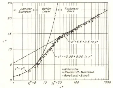
Fig. 1. Universal velocity profile (From Martinelli, 1947.)

2.1 Structure of a turbulent boundary layer and the law of the wall

In order to develop a mathematical/numerical framework that can reproduce the effects of near-wall turbulence on the flow, it is necessary to understand the character of near-near-wall turbulence and the structure of a turbulent boundary layer. The typical “layered” composition for a near-wall turbulent flow as found in a constant-pressure boundary layer, channel or pipe flow is shown in (Fig.1, 2) [Martinelli (1947); Clauser (1956)] . Although the thickness of this viscosity-affected zone is usually two or more orders of magnitude less than the overall width of the flow, its effects extend over the whole flow field since, typically, half of the velocity change from the wall to the free stream occurs in this region. This thin sub-layer and the adjacent transition region extending to the fully turbulent regime is a region where effective transport properties change at a rate typically two or more orders of magnitude faster than elsewhere in the flow.

For simple flows (boundary layer at zero pressure gradient and channel flows) two characteristic zones (Fig. 3) are considered in the numerical calculation of the near-wall region – the viscous sub-layer (“bridged” by wall functions) and the fully turbulent region (where

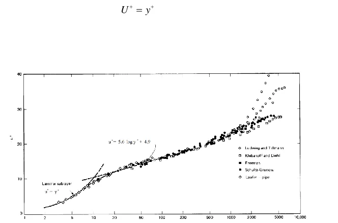
Uy (1)

Fig. 2. Universal wall law plot for turbulent boundary layers on smooth, solid surfaces (From Clauser, 1956.)

Across the fully turbulent region the dimensionless velocity is proportional to the logarithm of the dimensionless wall distance:

 

1 ln

U Ey



 _ 

(2)

The velocity and distance from the wall are non-dimensionalized as:

; yU ; w

U

U y U

U

  



 

 _  _{ }

(3)

The above equations represent best known and still widely used wall function (“standard wall functions”) for the momentum equation, more commonly known as the law of the wall

 



U  f y



.

2.2 Equilibrium assumptions

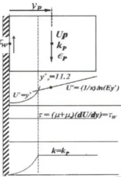
Fig. 3. Location of the near-wall node P with reference to viscous sub-layer and fully turbulent region

Fig. 4. Assumed profiles of dimensionless velocity, total shear stress and turbulent kinetic energy across the near-wall cell

Standard wall functions are based on several assumptions that are supposed to be valid throughout the fully turbulent near-wall layer (Fig. 4):

1. AtyyP, the mean velocity component parallel to the wall obeys the logarithmic law

of the wall (Eq. (2)).

2. The total shear stress remains constant across the near-wall cell and equal to the wall

shear stress ( v t w

U

uv const y

       

 )

3. The ratio of the turbulent shear stress and kinetic energy (known as the “structure parameter”) is presumed to be constant, i.e. 1 2

0.3

uv k C_

   (according to experimental data).

4. The turbulent kinetic energy is in local equilibrium, i.e. the net transport by convection and diffusion is negligible so that Pk (the generation of k is in equilibrium with the

destruction of k).

5. The turbulent length and time scales increase linearly across this flow region, i.e. 3 2

l

lk  C y and  k C y (where Cl  C3 4 and





1 2

These assumptions are reasonably well satisfied in simple wall flows such as the constant-pressure boundary layer, plane channel or pipe flow, as can be seen from numerous experiments and DNS databases [Kim (2011)]. On the basis of the above mentioned assumptions, approximate formulae are then supplied as the required input to the near-wall cell (for wall-shear stress, mean dissipation rate, turbulence-energy production rate, wall heat flux, etc). None of these assumptions can be relied on, however, in more complex flows that depart far from equilibrium.

2.3. Wall functions for momentum equation (for wall-parallel velocity)

In the near-wall control volume, for the velocity component parallel to the wall, the wall shear stress is obtained from the log-law (Eq. (2)):





ln P w P w U Ey        (4)

This implicit form of the wall function leads to very poor behavior in flows involving separation, stagnation and reattachment, where the wall shear stress falls to zero. One of the first improvements, proposed by [Launder and Spalding (1974)], was to replace the characteristic turbulent velocity scale  w by

1 4 1 2

C k on the basis of local equilibrium

condition, where k is evaluated at near-wall node (at y 30 , 2

0.3

U k ), leading to the

following expression for the wall shear stress:





1 4 1 2

1 4 1 2

ln

P P

w

P P

C k U

EC k y

      (5)

The above formula is applied if the near-wall node is within the fully-turbulent region, which is defined asy 11.63. If the viscous sub-layer is large in comparison to the width of

the near-wall cell



y11.63



, according to the linear-law (Eq. (1)), the expression for the wall shear stress is given by:

P w

P U

y

  (6)

2.4. Wall functions for turbulent kinetic energy equation

Boundary-layer solvers (which deal for the most part with flows near local equilibrium) usually adopt simply the local turbulent energy equilibrium values of the generation and dissipation terms evaluated at the near-wall node P. Since production and dissipation of turbulent kinetic energy are expected to vary greatly across the near-wall region, it is preferable to determine their cell-averaged values - average production, Pk ,and average dissipation,  - which take

into account the changes in turbulence quantities across the near-wall cell, by direct integration over the near-wall control volume. These averaged quantities are approximated differently in different wall functions and it is principally through changes in the assumed profiles of turbulent shear stress, turbulent kinetic energy and dissipation of turbulent kinetic energy used in expressions for Pk and, that improvements in the standard wall functions are achieved

2.4.1 Launder & Spalding (LS)

The average production of turbulent kinetic energy is calculated assuming a constant total shear stress across the near-wall cell and equal to the wall shear stress (

v t w

U

uv const y

       

 ). At the wall uv0and w U

y

 

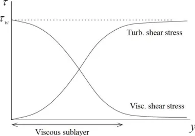
 . Across the viscous sub-layer the turbulent shear stress is negligible and the viscous shear stress is the dominant. Outside the thin viscous sub-layer, in the fully turbulent part of the boundary layer, molecular effects are negligible and the turbulent shear stress is essentially equal to the total shear stress. In the fully turbulent region of the zero pressure gradient boundary layer the turbulent shear stress is thus equal in magnitude to the wall shear stress, uvw (Fig. 5). In

internal fully developed flows, such as pipe or channel flows, the total shear stress varies linearly from w at the wall to the zero at symmetry axis or plane. At high mean flow Re

numbers the viscous sub-layer is thin enough for the reduction in shear stress across it to be negligible. The approximation of uniform total shear stress in the inner region is thus reasonable.

Fig. 5. Distribution of the total (viscous + turbulent) shear stress in the wall layers

The strain-rate ( U y) used in the cell-averaged production term is approximated from the nodal values of velocity and wall distance:

0

1 yn

P

k w

n P

U U

P uv dy

y  y  y



  





(7)

Likewise, the average dissipation rate is obtained by using the same assumptions employed in the evaluation of the average production rate:

3 4 3 2

P P

p C k U

y 





 (8)

2.4.2 Simplified Chieng & Launder (SCL)

next to a wall to be evaluated, the following assumptions are used [Chieng and Launder (1980); Johnson and Launder (1982)]:

1. The turbulent shear stress is zero in the viscous sub-layer, but constant (and equal to the wall shear stress) in the fully turbulent region.

2. The turbulent kinetic energy varies with wall distance according to the parabolic profile ( 2

2 k y const

   ) across the viscous sub-layer and is constant (and equal to

P

k ) in the fully turbulent region.

3. The dissipation of turbulent kinetic energy is constant in the viscous sub-layer and equal to its wall-limiting value ( 2

2 kP y

 

   ), while in the fully turbulent region



is assumed to vary inversely with wall distance



3 2







l

k C y

  .

Fig.6. Assumed profiles of turbulent shear stress, kinetic energy and dissipation rate across the near wall cell

2

1 4 1 2 1 4 1 2

0

1 1

ln

n n

y y

w w n

k w

y

n n P P n

y U

P uv dy dy

y y y  C k y C k y y

             _{ }  _{ }





(9)

3 2 3 2

2 0 2 2 1 1 ln n y y n

P P P P

y

n l n l

y

k k k k

dy dy

y y C y y y C y

         _  _       







   (10)

The sub-layer thickness,yis determined from assuming a constant sub-layer Reynolds number

( 1 2

20 P

R k y   ) andCl  C3 4 . Unlike the production rate (the velocity change across

the viscous sub-layer, whereuv0, does not contribute to generation of turbulence), the dissipation rate is non-zero in the viscous layer [Craft, Gerasimov, Iacovides and Launder (2002)].

2.5 Wall functions for dissipation rate equation

The transport equation for the dissipation of turbulent kinetic energy could be treated in a similar manner as the k equation. However, more common practice is to avoid integration over the near-wall cell, but to use its wall-equilibrium point value evaluated at the near-wall node P,

based on the linear length-scale variation with a distance from the wall ( 3 2 l

l k C y):

3 2 P P l P k C y

  (11)

3. Wall functions numerical implementation

3.1 Solution procedure

The numerical calculations are performed in in-house developed finite-volume-based elliptic code written in FORTRAN programming language. The governing partial differential equations are integrated by the finite-volume method over each of the finite control volumes in the flow domain and the resulting integrated transport equations are then discretized, using finite-difference-type formulas, to give a set of algebraic equations which are solved using an iterative method (TDMA). Coupling of the continuity equation and the momentum equations is done by using semi-implicit method for pressure-linked equations (SIMPLE) algorithm, while the stabilization of iteration procedure is provided by under-relaxation method. A staggered Cartesian grid is used with scalars stored at nodal positions and velocities at the cell faces. The hybrid-differencing scheme is used for the calculation of main coefficients in the discretized equations. Boundary conditions enter the discretized equations by suppression of the link to the boundary side and modifications of source terms. The appropriate coefficient of the discretized equation is set to zero and the boundary contribution is introduced through source terms sU and

P

s . In all cases considerable care has been taken to ensure that results are independent of the grid.

3.2 Momentum equation

modify the source term by introducing the boundary contribution, i.e. the replacement term, according to the following expression:

P w P A s U    (12) 3.3 k-equation

The k-equation is solved in the near-wall cell with modified production and dissipation terms (Eq. (7-10)). Introducing modified source terms into the k-equation is simply a matter of removing the old calculated near-wall cell values of production and dissipation, Pk and , from

the source term of the k-equation and then adding in the wall-function values. The wall function values for average production, P_k, and average dissipation rate, , are placed into source terms

U

s and sP as follows:





max , 0

U k

s  _ P  _Vol (13)





min k , 0

P P P s Vol k   _   

  (14)

3.4 ε -equation

To set the value ofP, source terms are added to the discretized equation as follows:

30 * 30

10 10

U P P

s   s   (15)

where 1030 is an arbitrary large number and P* is the wall function value for  at the near-wall node (Eq. (11). Substituting these source terms into the discretized equation leads to the following expression:



30



30 *

10 10

P P N N S S E E W W P

a   a  a a a    (16)

and, since the neighbouring coefficients aNN_, aSS _{are much smaller than}

30

10 _{, the}

expression becomes:

* P P

  (17)

4. Results and discussion

4.1 Fully developed channel flow

The test problem is the fully-developed plane channel flow at high Reynolds number (Fig.7). The results of the computations to test the standard wall functions in combination with the k



model are compared with the highest Reynolds number (Re=52000) of Laufer’s

transversal directions to ensure the independence of numerical results on the grid refinement. The calculations use sufficient lengths (120 half-widths) in the longitudinal direction to ascertain full flow development. Profiles of the streamwise velocity are presented in semi-logarithmic form in (Fig. 8). Both profiles agree well with the log-law: UAlogyB



A5.6 5.75; B4.9 5.5



in the inner layer.

The comparison of the computed and experimental turbulent kinetic energy profiles is presented in (Fig. 9). The predictions are in reasonably good agreement with the experimental data. The behavior of wall functions (LS and SCL) is almost identical in both cases.

Fig. 7. Fully-developed turbulent channel flow

Fig. 10. Turbulent flow past a backward facing step

4.2 Backward facing step flow

Turbulent flow past a backward facing step (Fig. 10) is chosen as a test case in an effort to resolve the variety of conflicting results that have been published concerning the performance of two-equation models and wall functions [Kim, Kline and Johnston (1980); Mansour, Kim and Moin (1983); Speziale and Tuan Ngo (1987)]. In a backward facing step flow, the flow faces a sudden expansion due to a step in the original channel and therefore non-equilibrium features are present. The flow separates at the corner and is characterized by the presence of a large recirculation region. The separated flow reattaches at a downstream location (L). The sudden step generates curved streamlines and recirculation zones (primary and secondary vortices) which are confined between the step and the reattachment point, which thus becomes a key parameter in such flows. Computations were conducted in a channel with an expansion ratio (H2 H13H 2H) of 3:2 at a Reynolds number of 46200 (based on the inlet centerline

Fig. 8. Comparison of velocity profiles computed with two standard wall functions (LS and SCL) and the linear kmodel to the log-law

Fig. 9. Comparison of profiles of the turbulent kinetic energy computed with two standard wall functions (LS and SCL) and the linear k model to experimental data of [Laufer (1951)]

The computed results of the standard wall functions in combination with the linear k

model are compared with experimental data for the backward-facing step flow investigated by [Kim, Kline and Johnston (1980)]. Computations are performed on four uniform meshes consisting of 400 x 40, 600 x 60, 800 x 80, and 1000 x 100 control volumes in the x and y

directions, respectively, and the grid 800 x 80 was selected as an optimal choice (Fig. 11).

The computed streamlines (Fig. 12) indicate a reattachment length in the range of 5.33 5.84

L  H, which underpredicts the experimental data of L7.0H.

Fig. 11. Grid independence study for backward facing step flow configuration (four uniform meshes; grid resolution: 400 x 40, 600 x 60, 800 x 80, and 1000 x 100)

profiles, the discrepancies are emphasized in the recirculating region, whereas in the recovery region the agreement is slightly better. In all cases there is no significant difference in the performance of wall functions (LS and SCL).

The results obtained in the case of the backward facing step flow configuration suggest that a proper solution of the problem might be found in modification of the standard kmodel [Chen and Kim (1987); Stevanović (2008)] and improvement of standard wall functions [Craft, Gant and Iacovides (2005) ], but this requires further analysis.

Fig. 13. Comparison of the calculated mean velocity profiles in the recirculating region



x7H



to the experimental data of [Kim, Kline, Johnston (1980)]

Fig. 14. Comparison of the calculated mean velocity profiles in the recovery region



x7H



Fig. 15. Comparison of computed turbulent kinetic energy profiles to experimental data of [Kim, Kline, Johnston (1980)] at two axial locations in recirculation region (up) and recovery

region (down)

5. Conclusion

The standard wall functions approach is formulated on the basis of assumed near-wall profiles of mean velocity (known as the law of the wall), turbulence quantities and temperature in local turbulent energy equilibrium. The assumed velocity and temperature profiles only correspond with actual profiles in simple shear flows at high Re numbers. Therefore, these assumptions are a limiting factor in complex non-equilibrium flows (separating and recirculating flows, flows with strong pressure gradients, rotating flows, flows where buoyant effects are significant etc.), where the velocity profiles are very different from the assumed ones. These premises are confirmed by the results in both analyzed cases – the simple flow configuration (fully developed channel flow) and complex flow configuration (backward facing step flow). However, a dillema remains about the main cause of discrepancies between computed and experimental results in the recirculating region of the backward facing step configuration.

sometimes mistakenly blame their difficulties on the use of non-optimum wall functions. This assessment is too often made when the wall functions are not the real cause of the problem. For example, the standard k model just doesn’t perform well for backward facing step flow. Many articles have appeared claiming that discrepancies between k model predictions and corresponding measurements for backstep problem are caused by wall functions.

Although the law of the wall and equilibrium assumptions are not valid in the recirculation region of the separating and reattaching flows, the general flow behaviour of backward-facing step flow is not significantly altered by the particular form of the wall functions. The results obtained in the case of the backward facing step flow configuration suggest that a solution of the problem could be found in modification of the standard kmodel and improvement of standard wall functions.

Nevertheless, the modification of linear kmodel is almost firmly established. Probably, more unexplored direction into the new investigations might be found in the improvement of standard wall functions, but this would require further analysis.

Acknowledgements

This work has been supported by the Republic of Serbia Ministry of Education, Science and Technological Development (Project: “Increase in Energy and Ecology Efficiency of Processes in Pulverized Coal-Fired Furnace and Optimization of Utility Steam Boiler Air Preheater by Using In-House Developed Software Tools”, No. TR-33018).

NOMENCLATURE

, , , , E W N S P

a - east, west, north etc. coefficients in

the discretized equations _kgs1

 

A - area of the cell face parallel to the wall _m2

 

l

C - constant in near-wall length-scale

definition

 



C - structure parameter

 



C - parameter in near-wall time-scale

definition _{m s}1 

 

E - roughness parameter

 



h - half-width of the channel (channel flow)

 

m

1

H - inlet channel height (step flow)

 

m

2

H - outlet channel height (step flow)

 

m

H - step height

 

m

k - turbulent kinetic energy _{m s}2 2

 

k

P - average production rate of turbulent

kinetic energy 2 3

m s

 

 

R - viscous sublayer Reynolds number

 



Re - Reynolds number

 



P

s - linearized source term

U

s - source term in the discretized equation

uv



 - Reynolds (turbulent) shear stress

_{kgm s}1 2

 

U - streamwise mean velocity component _ms1

 

0

U - free-stream velocity or inlet velocity

1

ms

 

 

U - friction velocity ms1 

 

 

l - turbulent length scale

 

m

L - reattachment length

 

m

k

P - production rate of turbulent kinetic

energy _{m s}2 3

 

 - rate of dissipation of turbulent kinetic energy _{m s}2 3

 

 - average rate of dissipation of turbulent kinetic energy _{m s}2 3

   - von Karman constant,  0.41

 

  - dynamic viscosity _{kgm s}1 1

 

 - kinematic viscosity _{m s}2 1

 

 - density _kgm3

 

 - total shear stress _{kgm s}1 2

  or turbulent time scale

 

s

t

 - turbulent shear stress _{kgm s}1 2

 

v

 - viscous shear stress _{kgm s}1 2

 

w

 - wall shear stress 1 2

kgm s 

 

 

 - general variable

Subscripts

, , ,

E W N S - node values of variables , , ,

e w n s - face values of variables

P - value at the near-wall node or current node

t - value in the fully turbulent region

y - distance from the wall

 

m

y - dimensionless distance from the wall

 



Greek symbols

 - boundary layer thickness

 

m

Vol

 - cell volume _m3

 

 - value at the edge of the viscous sublayer or in the viscous sublayer

w - wall value  - “friction” value

Superscripts

 - non-dimensional near-wall value scaled by

Acronyms

CFD - computational fluid dynamics

CPU - central processing unit

DNS - direct numerical simulation

LS - Launder & Spalding wall function

RANS - Reynolds-averaged Navier-Stokes

SIMPLE - semi-implicit method for pressure- linked equations

TDMA - tri-diagonal matrix algorithm

Извод

Процена и ограничења стандардних функција зида у каналу и

конфигурација корака протока

B. Stanković1, A. Stojanović1*, M. Sijerčić 1, S. Belošević1 and S. Čantrak2 1

Институт за нуклеарне науке „Винча“, Универзитет у Београду, Лабораторија за термотехнику и енергетику,

Поштански број 522, 11001 Београд, Србија 2

Машински факултет, Универзитет у Београду, Краљице Марије 16, 11120 Београд 35, Србија

* Главни аутор [email protected]

Резиме

Овај рад се бави истраживањем имплементације, процене и ограничења конвенционалних функција зида, на основу закона о зиду, у комбинацији са линеарном





k

турбуленцијом модела једноставних (потпуно развијен канал) и комплексних (повратних корака) конфигурација протока. Вискозност у близини зида – утиче на слој протока турбулентног флуида и поставља бројне изазове, како са гледишта моделирања тако и нумеричког гледишта. Преко овог танког зида суседне регије, својства турбуленције мењају ред величине брже него у остатку тока. Упркос закону зида и равнотеже претпоставке не важе у рециркулационом региону токова одвајања и прикључивања, опште понашање протока код протока са повратним корацима није битно измењено одређеним обликом стандардних зидних функција. Резултати добијени у случају конфигурације протока повратних корака указују да се решење може наћи у модификацији линеарног

k





модела и побољшања стандардних зидних функција.

Кључне речи:турбуленција, повратни кораци,

k





модел, функције зида

References

Amano RS, Jensen MK and Goel P (1983). A numerical and experimental investigation of turbulent heat transport downstream from an abrupt pipe expansion. Journal of Heat Transfer, 105:862-872.

Amano RS (1984). Development of a turbulence near wall model and its application to separated and reattached flows. Numerical Heat Transfer, 17:59-75.

Chen YS, Kim SW (1987). Computation of turbulent flows using an extended k



turbulence closure model. NASA Contractor Report 179204.

Chieng CC, Launder BE (1980). On the calculation of turbulent heat transport downstream from an pipe expansion. Numerical Heat Transfer 3:189-207.

Craft TJ, Gerasimov AV, Iacovides H, Launder BE (2002). Progress in the generalization of wall-function treatments. International Journal of Heat and Fluid Flow 23:148-160. Craft TJ, Gant SE and Iacovides H (2005). Application of a generalized RANS wall function to

recirculating flows with heat transfer. Proceedings of 4th International Conference on Computational Heat and Mass Transfer. May 17-20, Paris-Cachan, France.

Demuren AO, Sarkar S (1993). Perspective: systematic study of Reynolds stress closure models in the computation of plane channel flows. Journal of Fluids Engineering 115:5-12. Gant S (2002). Development and application of a new wall function for complex turbulent

flows. Ph. D. Thesis. University of Manchester Institute of Science and Technology, Manchester, United Kingdom

Gerasimov A (2003). Development and validation of analytical wall-function strategy for modeling forced, mixed and natural convection flows. Ph. D. Thesis. University of Manchester Institute of Science and Technology, Manchester, United Kingdom.

Hanjalić K, Launder BE (2011). Modelling Turbulence in Engineering and the Environment: Second-Moment Routes to Closure. Cambridge University Press.

Hanjalić K, Jakirlić S (2002). Second-Moment Turbulence Closure Modeling. Closure Strategies for Turbulent and Transitional Flows edited by B.E. Launder and N.D. Sandham. Cambridge University Press, 47-101.

Johnson RW, Launder BE (1982). Discussion of “On the Calculation of Turbulent Heat Transport downstream from an Abrupt Pipe Expansion”. Numerical Heat Transfer, Technical Note, 5:493-496.

Kiel R, Vieth D (1995). Experimental and theoretical investigation of the near-wall region in a turbulent separated and reattached flow. Experimental Thermal and Fluid Sciences 11:243-256.

Kim J, Kline SJ, Johnston JP (1980). Investigation of separation and reattachment of a turbulent shear layer: flow over a backward-facing step. Journal of Fluids Engineering 102:302-308. Kim J (2011). Progress in pipe and channel flow turbulence, 1961-2011. Turbulence

Colloquium Marseille 2011. September 26-30, 2011, Marseille, France.

Kim SE, Choudhury D (1995). A Near-Wall Treatment Using Wall Functions Sensitized to Pressure Gradient. FED , Separated and Complex Flows, ASME 217:273-280.

Laufer J (1951). Investigation of turbulent flow in a two-dimensional channel. NACA Report 1053.

Launder BE, Spalding DB (1974). The numerical computation of turbulent flows. Computer Methods in Applied Mechanics and Engineering 3:269-289.

Mansour NN, Kim J, Moin P (1983). Computation of turbulent flows over a backward-facing step. NASA Technical Memorandum 85851.

Martinelli RC (1947). Heat transfer to molten metals. Trans. ASME 69:947-959.

Patankar SV, Spalding DB (1967). Heat and Mass Transfer in Boundary Layers. Morgan-Grampian Press.

Sijerčić M (1998). Matematičko modeliranje kompleksnih turbulentnih transportnih procesa. Jugoslovensko društvo termičara i Institut za nuklearne nauke “Vinča”. (Mathematical

Modelling of Complex Turbulent Transport Processes. Yugoslav Society of Heat Transfer Engineers and Institute of Nuclear Sciences “Vinča”.) (in Serbian)

Speziale CG, Tuan Ngo (1987). Numerical solution of turbulent flow past a backward facing step using a nonlinear

k





model. ICASE Report No. 87-74.