Posterior Regularization for Learning with Side Information and Weak Supervision

University of Pennsylvania

ScholarlyCommons

Publicly Accessible Penn Dissertations

Fall 12-22-2010

Posterior Regularization for Learning with Side

Information and Weak Supervision

Kuzman Ganchev

University of Pennsylvania, [email protected]

Follow this and additional works at:http://repository.upenn.edu/edissertations

Part of theArtificial Intelligence and Robotics Commons, and theStatistical Models Commons

This paper is posted at ScholarlyCommons.http://repository.upenn.edu/edissertations/265

For more information, please [email protected].

Recommended Citation

Ganchev, Kuzman, "Posterior Regularization for Learning with Side Information and Weak Supervision" (2010).Publicly Accessible Penn Dissertations. 265.

Posterior Regularization for Learning with Side Information and Weak

Supervision

Abstract

Supervised machine learning techniques have been very successful for a variety of tasks and domains including natural language processing, computer vision, and computational biology. Unfortunately, their use often requires creation of large problem-specific training corpora that can make these methods prohibitively expensive. At the same time, we often have access to external problem-specific information that we cannot alway easily incorporate. We might know how to solve the problem in another domain (e.g. for a different language); we might have access to cheap but noisy training data; or a domain expert might be available who would be able to guide a human learner much more efficiently than by simply creating an IID training corpus. A key challenge for weakly supervised learning is then how to incorporate such kinds of auxiliary information arising from indirect supervision.

In this thesis, we present Posterior Regularization, a probabilistic framework for structured, weakly supervised learning. Posterior Regularization is applicable to probabilistic models with latent variables and exports a language for specifying constraints or preferences about posterior distributions of latent variables. We show that this language is powerful enough to specify realistic prior knowledge for a variety applications in natural language processing. Additionally, because Posterior Regularization separates model complexity from the complexity of structural constraints, it can be used for structured problems with relatively little computational overhead. We apply Posterior Regularization to several problems in natural language processing including word alignment for machine translation, transfer of linguistic resources across languages and grammar induction. Additionally, we find that we can apply Posterior Regularization to the problem of multi-view learning, achieving particularly good results for transfer learning. We also explore the theoretical relationship between Posterior Regularization and other proposed frameworks for encoding this kind of prior knowledge, and show a close relationship to Constraint Driven Learning as well as to Generalized Expectation

Constraints.

Degree Type

Dissertation

Degree Name

Doctor of Philosophy (PhD)

Graduate Group

Computer and Information Science

First Advisor

Fernando Pereira

Second Advisor

Ben Taskar

Keywords

Posterior Regularization Framework, Unsupervised Learning, Latent Variable Models, Prior Knowledge, Natural Language Processing, Machine Learning, Partial Supervision

Subject Categories

Artificial Intelligence and Robotics | Computer Sciences | Statistical Models

POSTERIOR REGULARIZATION FOR

LEARNING WITH SIDE INFORMATION AND

WEAK SUPERVISION

Kuzman Ganchev

A DISSERTATION

in

Computer and Information Science

Presented to the Faculties of the University of Pennsylvania

in

Partial Fulfillment of the Requirements for the

Degree of Doctor of Philosophy

2010

Fernando Pereira, Professor of Computer and Information Science Supervisor of Dissertation

Ben Taskar, Assistant Professor of Computer and Information Science Supervisor of Dissertation

Jianbo Shi, Associate Professor of Computer and Information Science Graduate Group Chairperson

Dissertation Committee

Michael Collins, Associate Professor of Computer Science, MIT

Mark Liberman, Professor of Phonetics Department of Linguistics

Mitch Marcus, Professor of Computer and Information Science

Posterior Regularization for Learning with Side Information and Weak Supervision

COPYRIGHT

2010

This thesis is dedicated to my parents, who have given me everything.

Acknowledgements

Thanks . . .

To my advisors Fernando Pereira and Ben Taskar. Fernando was my first advisor at

Penn and has been a source of inspiration from the start. It seems that no matter how well

I think I understand a problem, Fernando can shed new light on it. His advice is always

invaluable, and more often than not surprising. He seems to know relevant literature in

areas I would never have believed to be related, and to find bugs, as if by magic, in code he

has never seen. Ben was my advisor since shortly after he joined Penn. None of the work

presented here would have been conceived, implemented, tested, or described were it not

for him. “Ask Ben” seems to be a universal solution, and one of the hardest things about

leaving will be losing the ability to drop by his office to find out how to formalize, optimize

and visualize my ideas. Both Ben and Fernando are amazing people that have created a

friendly, warm, stress-free atmosphere that has made my years at Penn so enjoyable, and I

might never be able to repay them fully for all they have done for me.

To my committee: Mitch Marcus, Mike Collins, Mark Liberman, and Lyle Ungar for

their feedback, and support. Thanks to Mitch for agreeing to chair my committee and for

telling me what isn’t obvious – Chapter 5 was largely his idea. Mitch was never formally

my advisor, but he often played the part and I always felt welcome to ask for his advice and

support. Thanks to Mike for the very helpful, detailed comments and suggestions on both

the proposal and the thesis documents, and for agreeing to come in person both times. Mark

provided much needed linguistic perspective and suggested new applications and avenues,

that I would never have thought of. Thanks to Lyle for the very helpful comments both at

the proposal and at the defense. Without your direction this dissertation would have been

To Michael Kearns for showing me the world of finance, what it means to be clear,

and that it is possible to finish before the deadline. To Kiril Simov for giving me the

opportunity to do research in my native Bulgaria, where the work on Chapter 10 took place.

To Tia Newhall, who introduced me to research when I was an undergraduate, and who is

my first co-author. And to Richard Wicentowski, who introduced me to natural language

processing.

To the co-authors of the work in this dissertation. To João Graça, who is a partner for

the work in almost every chapter of this thesis, and who is usually responsible for more than

half of the energy in every project. To Jennifer Gillenwater who is a partner on all the

pars-ing chapters, and who writes the neatest, prettiest code I have ever seen. To John Blitzer,

who is a partner on the multi-view chapter (John – gl, hf). To my other collaborators, and

especially to Kedar Bellare, Steven Carroll, Koby Crammer, Mark Dredze, Ryan Gabbard,

Georgi Georgiev, Yang Jin, Alex Kulesza, Qian Liu, Mark Mandel, Gideon Mann, Andrew

McCallum, Ryan McDonald, Vassil Momchev, Preslav Nakov, Yuriy Nevmyvaka, Deyan

Peychev, Angus Roberts, Partha Pratim Talukdar, Jinsong Tan, Jennifer Wortman Vaughan,

and Peter White.

To the administrative staff, who are truly remarkable and especially to Mike Felker,

who has been voted “most useful person” in every informal poll. Thank you for running

the place so smoothly, keeping our lives simple, and always finding a way to resolve our

crises.

To Aaron, Alex, Alex, Alex, Axel, Brian, Cheryl, David, Dimo, Drew, Emily, Gabe,

Galia, Hannah, Iliana, Irena, Jeff, Jenn, Jenny, João, Julie, Karl, Lauren, Mike, Nick,

Partha, Qian, Rachel, Sophie, Wynn, for all the love, laughter, hugs, parties, dinners, drinks,

mafia games, D&D&D, zip-boing. Thank you for making these past six years so great.

Finally, to my mother, who nurtured my creativity and always cleaned up after my

early “science experiments”; to my father who taught me that everything is possible and to

strive for the best; to my brother without whose help I would never have gotten into any

university and who was always kind even when I was a brat; and to my love who makes

ABSTRACT

Posterior Regularization for Learning with Side Information and Weak Supervision

Kuzman Ganchev

Supervisors: Fernando Pereira and Ben Taskar

Supervised machine learning techniques have been very successful for a variety of tasks

and domains including natural language processing, computer vision, and computational

biology. Unfortunately, their use often requires creation of large problem-specific training

corpora that can make these methods prohibitively expensive. At the same time, we often

have access to external problem-specific information that we cannot alway easily

incorpo-rate. We might know how to solve the problem in another domain (e.g. for a different

language); we might have access to cheap but noisy training data; or a domain expert might

be available who would be able to guide a human learner much more efficiently than by

simply creating an IID training corpus. A key challenge for weakly supervised learning is

then how to incorporate such kinds of auxiliary information arising from indirect

supervi-sion.

In this thesis, we present Posterior Regularization, a probabilistic framework for

struc-tured, weakly supervised learning. Posterior Regularization is applicable to probabilistic

models with latent variables and exports a language for specifying constraints or

pref-erences about posterior distributions of latent variables. We show that this language is

powerful enough to specify realistic prior knowledge for a variety applications in natural

language processing. Additionally, because Posterior Regularizationseparatesmodel

com-plexity from the comcom-plexity of structural constraints, it can be used for structured problems

with relatively little computational overhead. We apply Posterior Regularization to several

problems in natural language processing including word alignment for machine translation,

transfer of linguistic resources across languages and grammar induction. Additionally, we

find that we can apply Posterior Regularization to the problem of multi-view learning,

re-lationship between Posterior Regularization and other proposed frameworks for encoding

this kind of prior knowledge, and show a close relationship to Constraint Driven Learning

Contents

1 Introduction 1

1.1 Contributions . . . 4

1.2 Thesis Overview . . . 5

1.2.1 Mathematical Formulation, Intuitions and Related Methods . . . 5

1.2.2 Applications and Experimental Results . . . 6

I

Mathematical Formulation, Intuitions, Related Methods

7

2.2 Regularization via Posterior Constraints . . . 10

2.3 Slack Constraints vs. Penalty . . . 14

2.3.1 Computing the Posterior Regularizer . . . 14

2.4 Factored q(Y) for Factored Constraints . . . 15

2.5 Generative Posterior Regularization via Expectation Maximization . . . 16

2.6 Penalized Slack via Expectation Maximization . . . 20

2.7 PR for Discriminative Models . . . 20

3 Summary of Applications 23 4 Related Frameworks 27 4.1 Constraint Driven Learning . . . 27

4.3 Measurements in a Bayesian Framework . . . 30

5 Expressivity of the Language 34 5.1 Preliminaries . . . 35

5.1.1 Decomposable constraints . . . 37

5.2 Feature labeling . . . 38

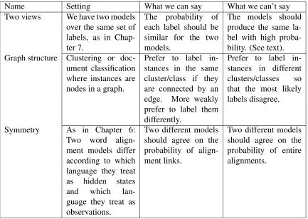
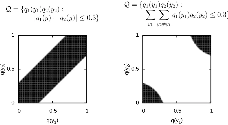
5.3 Agreement and Disagreement . . . 40

5.3.1 Two Views . . . 40

5.3.2 Graph Structure . . . 43

5.3.3 Symmetry . . . 45

5.4 Sparsity Structure . . . 47

5.5 Sequence Models . . . 49

5.6 Trees . . . 53

5.6.1 Depth and Branching Factor . . . 54

5.6.2 Siblings . . . 58

5.6.3 Almost Projective . . . 61

5.6.4 Grandparents and Grandchildren . . . 63

II Empirical Study

66

6.2 Bijectivity Constraints . . . 70

6.3 Symmetry Constraints . . . 71

6.4 Results . . . 72

7 Mutli-view learning 75 7.1 Stochastic Agreement . . . 76

7.2 Partial Agreement and Hierarchical Labels . . . 79

7.3 Relation to Other Multi-View Learning . . . 81

8 Cross lingual projection 86

8.1 Approach . . . 87

8.2 Parsing Models . . . 89

8.3 Experiments . . . 90

8.4 Results . . . 91

8.5 Generative Parser . . . 92

8.6 Discriminative Parser . . . 94

9 Enforcing sparsity structure for POS induction 95 9.0.1 l1/linf Regularization for POS . . . 96

9.1 Results . . . 98

10 Enforcing sparsity structure for Grammar induction 102 10.1 Parsing Model . . . 103

10.1.1 Dependency Model With Valence (DMV) . . . 104

10.1.2 Model Extensions . . . 105

Extending Stop Probabilities . . . 105

Extending Dependent Probabilities . . . 106

Complete Model . . . 106

10.1.3 Model Initialization . . . 107

10.2 Previous Learning Approaches . . . 108

10.2.1 Expectation Maximization . . . 109

10.2.2 Bayesian Learning . . . 109

Sparsity-Inducing Priors . . . 109

Parameter-Tying Priors . . . 112

10.2.3 Other Learning Approaches . . . 113

10.3 Learning with Sparse Posteriors . . . 114

10.3.1 L1Lmax Regularization . . . 114

10.4 Experiments . . . 117

10.4.1 Corpora . . . 117

10.4.3 Comparison with Previous Work . . . 121

10.4.4 Multilingual Results . . . 124

10.5 Analysis . . . 129

10.5.1 Instability . . . 129

10.5.2 Comparison of EM, PR, and DD Errors . . . 129

10.5.3 English Corrections . . . 131

10.5.4 Bulgarian Corrections . . . 133

10.6 Chapter Summary . . . 135

11 Conclusion 137 11.1 Future Directions . . . 137

11.1.1 New Applications . . . 138

11.1.2 Empirical Comparison . . . 139

11.1.3 New Kinds of Constraints . . . 139

11.1.4 Theoretical Analysis . . . 140

III Appendices

141

A.2 Estimation and Priors . . . 144

A.3 Structured Models . . . 145

A.4 Maximum Entropy and Maximum Likelihood . . . 146

B Scaling the strength of PR 148

C Proof of Proposition 2.1 149

List of Figures

1.1 Two examples of structured models we will use in this work. . . 2

1.2 Example part of speech induction application. . . 4

2.1 The PR objective for generative models as a sum of two KL terms. . . 13

2.2 Modified EM for optimizing generative PR objective . . . 17

4.1 The Bayesian model of Liang et al. [2009] using our notation. . . 31

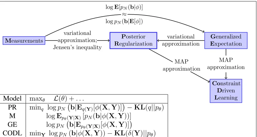
4.2 Summary of relationship between PR and related models. . . 33

5.1 Summary of the simplified constraints. . . 36

5.2 Illustration of two constraints for multi-view agreement. . . 43

5.3 Example of why grandparent/grandchild relationships cannot be captured. . . . 56

5.4 Example of why sibling relationships cannot be captured. . . 59

5.5 The additional non-projective tree possible by the parameters in Figure 5.4. . . 61

5.6 Example of why grandparent relationships cannot be captured. . . 64

6.1 Posterior distributions of an En-Fr sentence. . . 69

6.2 Precision/Recall curves: EM vs PR (Bijective and Symmetric constraints) . . . 73

7.1 Illustration of different two-view loss functions. . . 81

8.1 Example sentence for grammar induction via bitext projection . . . 87

8.2 Learning curves for grammar induction via bitext projection . . . 92

8.3 Posteriors of parse edges: how bitext projection helps. . . 93

9.2 Experimental results for posterior vs parameter sparsity in POS tagging. . . 100

10.1 Example of a dependency tree with DMV probabilities. . . 104

10.2 Comparison of parameters for a max likelihood DMV and an EM-trained DMV

for English. . . 110

10.3 The digamma function. . . 111

10.4 The`1/`∞regularization term for a toy example. . . 115

10.5 Accuracy and negative log likelihood on held out development data as a

func-tion of the training iterafunc-tion for the DMV. . . 120

10.6 Directed accuracy and negative log likelihood on held-out development data as

a function of the training iteration for the E-DMV model with the best

param-eter setting. . . 121

10.7 Difference in accuracy between the sparsity inducing training methods and EM

training for the DMV model across the 12 languages. . . 127

10.8 Difference in accuracy between PR training with the different constraints and

DD for the DMV model across the 12 languages. . . 127

10.9 Comparing the different sparsity constraints for the DMV model over twelve

different languages. . . 128

10.10Difference in accuracy between the sparsity inducing training methods and EM

training for the E-DMV model with the different training method across the 12

languages. . . 128

10.11The accuracy overall and for different POS tag types in the English corpus as a

function of`1/`∞as we vary the constraint strength. . . 129

List of Tables

2.1 Summary of notation used. . . 10

3.1 Summary of applications of Posterior Regularization we describe . . . 23

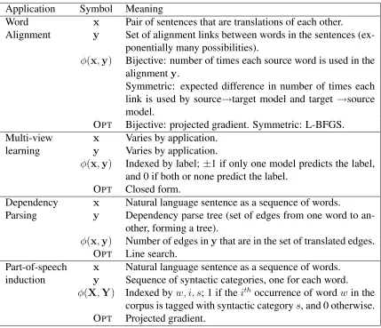
3.2 Summary of variable and constraint meanings for applications. . . 24

5.1 Summary of some factorizable agreement constraints . . . 41

5.2 Summary of simple constraints that are possible for sequences. . . 50

5.3 Summary of simple constraints that are decomposable for trees. . . 55

5.4 Summary of some natural constraints that are not feasible for trees. . . 56

7.1 Performance of transfer learning on a sentiment classification. . . 83

7.2 Results of two view learning for named entity disambiguation. . . 84

7.3 F-1 scores for noun phrase chunking with context/content views. . . 85

8.1 Features used by the MSTParser. . . 90

8.2 Accuracy values at the 10k training sentences point of Figure 8.2. . . 92

9.1 Posterior sparsity corpus statistics. . . 98

10.1 Corpus statistics for sentences with lengths≤10, after stripping punctuation. . 118

10.2 Directed attachment accuracy results on the test corpus (for sentences of lengths ≤10, no punctuation). . . 118

10.3 Directed attachment accuracy results on the test corpus. . . 119

10.4 Comparison with previous published results for dependency parsing. . . 122

10.5 Attachment accuracy results. . . 126

Chapter 1

Introduction

Machine learning in general and statistical models in particular have found applications in

a wide variety of domains, across a range of disciplines including natural language

process-ing, computer vision, signal processprocess-ing, computational finance medical image analysis and

computational biology to name just a few. For many of these application domains the most

successful models use supervised machine learning approaches that require large quantities

of annotated data in order to build models able to perform well.1

In some situations, the annotations necessary for applying supervised learning

algo-rithms occur naturally or can be obtained relatively inexpensively. For example, if we

would like to predict the price and volatility of stocks, bonds or futures contracts, we can

obtain historical data relatively inexpensively. This data can then be used to train

predic-tors for use in the future. Similarly, machine translation systems are typically trained using

already available corpora such as parliamentary proceedings that have to be available in

multiple languages by law. In contrast to these relatively data-abundant applications, for

the vast majority of applications the successful application of machine learning techniques

requires expensive manual annotation. For example, in order to train a state of the art

named entity recognition system thousands of sentences must be annotated for the

enti-ties of interest. A similar situation exists for other machine learning applications such as

syntactic analysis of natural language, coreference resolution, relation extraction, object

recognition, gene finding, handwriting recognition and speech recognition.

Use

V

good

ADJ

grammarsN

1 1 2 3

we know the way

sabemos el camino null

Figure 1.1: Two examples of structured models we will use in this work. Left: a depen-dency tree representation of syntax. The hidden variables are the identities of the edges that compose the tree. Right: a hidden Markov model used for word alignment. The hidden variables are the identities of the source language words that are translations of the target language words.

This annotation process is often the most time-consuming and expensive part of the

construction of usable model. For example, 400 hours were needed to label a single hour

of speech at the phonetic level [Greenberg, 1996]. The Penn Chinese Treebank project

released the first version of its 4,000 sentences two years after the project began [Hwa

et al., 2005]. Furthermore, to achieve optimal performance, we need a separate corpus for

each domain of interest. For example, syntactic parsers trained on news perform poorly on

biomedical test [Dredze et al., 2007]. As the number of tasks, languages and target domains

of interest increases hand-labeling quickly becomes prohibitively slow and expensive.

For many problems where it is expensive to create annotations, unannotated data are

abundant. For example, natural language text in many domains is widely available,

se-quenced genomes for many organisms can be downloaded from public databases, and large

collections of images are much easier to obtain than annotated images. In order to

ex-ploit this inexpensive data, a variety of unsupervised machine learning approaches have

been devised. In unsupervised problems where data has sequential, recursive, spatial,

re-lational, and other kinds of structure, we often employ structured statistical models with

latent variables to tease apart the underlying dependencies and induce meaningful

seman-tic categories. Unsupervised part-of-speech and grammar induction, and word and phrase

alignment for statistical machine translation in natural language processing are examples

of such aims. Generative models (probabilistic grammars, graphical models, etc.) are

hidden variables, typically via the Expectation Maximization (EM) algorithm. Figure 1.1

shows a couple of examples of the model structures that we deal with in this dissertation.

Because of computational and statistical concerns, generative models used in practice

are very simplistic models of the underlying phenomena; for example, the syntactic

struc-ture of language or the language translation process. A pernicious problem with such

mod-els is that marginal likelihood may not guide the model towards the intended role for the

latent variables, instead focusing on explaining irrelevant but common correlations in the

data. Since we are mostly interested in the distribution of the latent variables in the hope

that they capture intended regularities without direct supervision, controlling this latent

distribution is critical. Less direct methods such as clever initialization, ad hoc procedural

modifications, and complex data transformations are often used to affect the posteriors of

latent variables in a desired manner. As an example, in the problem of part of speech

in-duction, the goal is to derive a set of syntactic categories from unannotated text. Because

of computational complexity and our limited understanding of how children learn

syntac-tic categories, this problem is typically solved using maximum likelihood training and a

hidden Markov model. As we see in Figure 1.2 (left panel), maximum likelihood training

results in very high ambiguity for each word. Depending on context, the hidden Markov

model might label the word “China” as a “noun”, “verb”, or “preposition.”

A key challenge for structured, weakly supervised learning is developing a flexible,

declarative framework for expressing structural constraints on latent variables arising from

prior knowledge and indirect supervision. Structured models have the ability to capture a

very rich array of possible relationships, but adding complexity to the model often leads

to intractable inference. In this dissertation, we present the posterior regularization (PR)

framework, which separates model complexity from the complexity of structural

con-straints it is desired to satisfy. Unlike parametric regularization in a Bayesian framework,

our approach incorporates data-dependent constraints that are easy to encode as

informa-tion about modelposteriorson the observed data, but may be difficult to encode as

infor-mation about model parameters through Bayesianpriors. In the right panel of Figure 1.2

we see that by imposing an appropriate penalty for the ambiguity of each word, we

PREP

TO

V

N

DET

ADJ

hire (3.4)

merge (2.8)

run (5.8)

china (7.6)

u.s. (7.9)

PREP

TO

V

N

DET

ADJ

hire (1.0)

merge (1.1)

run (2.5)

china (1.1)

u.s. (1.9)

Maximum Likelihood Posterior Regularization

Figure 1.2: Example part of speech induction application. In each panel words are on the right and parts of speech on the left. A link mean that the word was automatically tagged with that part of speech in some context. The numbers in parentheses indicate a measure of the tag-ambiguity of each word (see Chapter 9 for details). Left: conventional maximum likelihood training. Right: the method proposed in this work. See text for explanation.

categories. The experiments that produced Figure 1.2 are described in Chapter 9.

Chap-ters 5 and 6-10 describe a variety of such useful prior knowledge constraints in several

application domains.

1.1

Contributions

This thesis deals with the problem of incorporating prior knowledge into unsupervised

and semi-supervised learning for structured and unstructured models. We focus on

mod-els where exact efficient inference is possible, and describe a framework for efficiently

incorporating prior knowledge into both generative and discriminative models, both for

structured and unstructured data. Specifically, we present:

• A flexible, declarative framework for structured, weakly supervised learning via

pos-terior regularization.

• An efficient algorithm for model estimation with posterior regularization.

• An extensive evaluation of different types of constraints in several domains:

part-of-speech induction, unsupervised grammar induction and bitext word alignment.

• A detailed explanation of the connections between several other recent propos-als for weak supervision, including structured constraint-driven learning [Chang

et al., 2007], generalized expectation criteria [Mann and McCallum, 2008, 2007]

and Bayesian measurements [Liang et al., 2009].

1.2

Thesis Overview

This section describes the general organization of the thesis. Part I of the document

de-scribes the mathematical formulation of the posterior regularization framework, tries to

give some intuitions about the kinds of knowledge that can efficiently be incorporated into

the framework for a variety of models, and describes how posterior regularization is related

to a few recently proposed frameworks that try to encode similar kinds of prior

knowl-edge. Part II of the document describes applications of posterior regularization for with

associated experimental results. Chapter 11 concludes the dissertation.

1.2.1

Mathematical Formulation, Intuitions and Related Methods

Chapter 2 describes the posterior regularization (PR) framework as a mathematical

formu-lation. Section 2.2 describes the objective we optimize and Sections 2.5 and 2.7 describe

a simple algorithm to perform the optimization for generative and discriminative models.

Chapter 3 previews the applications described in Part II. Chapter 4 relates the PR

frame-work to several related methods: Constraint Driven Learning [Chang et al., 2007, 2008]

in Section 4.1, Generalized Expectation Criteria [Mann and McCallum, 2007, 2008, 2010]

in Section 4.2 and Bayesian Measurements [Liang et al., 2009] in Section 4.3. Figure 4.2

summarizes the relationship between these frameworks. Chapter 5 attempts to give an

intu-ition for the kinds of prior knowledge that can be efficiently encoded in the PR framework,

1.2.2

Applications and Experimental Results

In Part II of the thesis, we present a series of experiments using the PR framework in a

variety of natural language application domains. Chapter 6 focuses on the problem of

un-supervised statistical word alignment, and trying to enforce that alignments should usually

be bijective and symmetric. Chapter 7 describes how the PR framework can be used for

multi-view learning, resulting in a closed-form projection and a Bhattacharyya distance

co-regularizer in two view learning. Chapter 8 describes experiments in projecting a

de-pendency grammar from one language to another by using a bilingual text. Chapters 9

and 10 describe how PR can be used to induce a sparsity structure for the induction of

syn-tactic analyses: part-of-speech induction in Chapter 9 and dependency grammar induction

Part I

Mathematical Formulation, Intuitions,

Chapter 2

Posterior Regularization Framework

In this chapter we describe the posterior regularization framework, which incorporates

side-information into parameter estimation in the form of linear constraints on posterior

expec-tations. 1 _{As we will show, this allows tractable learning and inference even when the}

constraints would be intractable to encode directly in the model parameters. By defining

a flexible language for specifying diverse types of problem-specific prior knowledge, we

make the framework applicable to a wide variety of probabilistic models, both generative

and discriminative. In Sections 2.1-2.6 we will focus on generative models, and describe

the case of discriminative models in Section 2.7. We will use a problem from natural

lan-guage processing as a running example in the exposition:

Running Example The task is part-of-speech (POS) tagging with limited or no

training data. Suppose we know that each sentence should have at least one verb

and at least one noun, and would like our model to capture this constraint on the

un-labeled sentences. The model we will be using is a first-order hidden Markov model

(HMM).

We describe four other applications with empirical results in Chapters 6-10, but it will

be easier to illustrate key concepts using this simple example.

2.1

Preliminaries and Notation

We assume that there is a natural division of variables into “input” variablesxand “target”

variables y for each data instance, where x’s are always observed. We denote the set

of all instances of unlabeled data as X. In case of semi-supervised learning, we have

some labeled data as well, and we will use the notation(XL,YL)to denote all the labeled

instances.

The starting point for using the PR framework is a probabilistic model. Let θ be the

parameters of the model. For now we assume a generative model pθ(x,y), and we use

L(θ) = logpθ(XL,YL) + logP_Ypθ(X,Y) + logp(θ)to denote the parameter-regularized log-likelihood of the data.

Running Example In the POS tagging example from above, we would use

x = {x1, x2, . . . x|x|} to denote a sentence (i.e. a sequence of words) and y =

{y1, y2, . . . y|x|}to denote a possible POS assignment. Using an HMM, it is defined

in the normal way as:

pθ(x,y) = |x|

Y

i=1

pθ(yi|yi−1) pθ(xi|yi)

with θ representing the multinomial distributions directly, and where pθ(y1|y0) =

pθ(y1) represents a set of initial probabilities. Suppose we have a small labeled

corpus and a larger unlabeled corpus. For a generative model such as an HMM, the

log-likelihood (+ log-prior) is:

L(θ) = logpθ(XL,YL) + log

X

Y

pθ(X,Y) + logp(θ),

where corpus probabilities are products over instances: pθ(XL,YL) =

Q

pθ(x,y)

and analogously forXL,YL; and wherep(θ)is a prior distribution over the

Symbol Meaning

x (observed) input variables for a particular example

y (usually hidden) output variables for a particular example

X,Y xandyfor the entire unlabeled portion of the corpus

XL,YL xandyfor the entire labeled portion of the corpus (possibly empty) pθ(x,y) a generative, joint model with parametersθ

L(θ) data log-likelihood and parameter prior:

logpθ(XL,YL) + logP_Ypθ(X,Y) + logp(θ)

Qx,Q posterior regularization set: constrained set of desired data-conditional

distributions φ(x,y) constraint features: used to encode posterior regularization

b bounds on the desired expected values of constraint features ξ slack variables used to allow small violations of constraints JQ(θ) posterior regularized likelihood: L(θ)−KL(Q kpθ(Y|X))

Table 2.1: Summary of notation used.

2.2

Regularization via Posterior Constraints

The goal of the posterior regularization framework is to restrict the space of the model

posteriors on unlabeled data as a way to guide the model towards desired behavior. In

this section we describe a version of PR specified with respect to a set of constraints. In

this case, posterior information is specified with sets Qof allowed distributions over the hidden variables y. We will define Qin terms of constraint features φ(X,Y) and their expectations.2

Running Example Recall that in our running example, we want to bias

learn-ing so that each sentence is labeled to contain at least one verb. To encode this

formally, we define a feature φ(x,y) = “number of verbs iny”, and require that

this feature has expectation at least 1. For consistency with the rest of the

expo-sition and standard optimization literature, we will use the equivalent φ(x,y) =

2_{Note: the constraint features do not appear anywhere in the model. If the model has a log-linear form,}

then it would be defined with respect to a different set ofmodelfeatures, not related to theconstraintfeatures

“negative number of verbs iny” and require this has expectation at most -1:3

Qx={qx(y) : Eq[φ(x,y)]≤ −1}

Note that we enforce the constraint only in expectation, so there might be a labeling

with non-zero probability that does not contain a verb. To actually enforce this

con-straint in the model would break the first-order Markov property of the distribution.

4 _{In order to also require at least one noun per sentence in expectation, we would}

add another constraint feature, so thatφwould be a function fromx,ypairs to_R2.

We defineQ, the set of valid distributions, with respect to theexpectationsof constraint features, rather than their probabilities, so that our objective leads to an efficient algorithm.

As we will see later in this section, we also require that the constraint features decompose

as a sum in order to ensure an efficient algorithm. More generally than in the running

example, we will define constraints over an entire corpus:

Constrained Posterior Set: Q={q(Y) :Eq[φ(X,Y)]≤b}. (2.1)

In words,Qdenotes the region where constraint feature expectations are bounded byb. Additionally, it is often useful to allow small violations whose norm is bounded by≥0:

Constrained Set(with slack) : Q={q(Y) :∃ξ, Eq[φ(X,Y)]−b≤ξ; ||ξ||_β ≤}. (2.2)

Hereξis a vector of slack variables and||·||_β denotes some norm. Note that the PR method we describe will only be useful ifQis non-empty:

Assumption 2.1. Qis non-empty.

We explore several types of constraints in Chapters 6-10, including: constraints similar

to the running example, where each hidden state is constrained to appear at most once in

expectation; constraints that bias two models to agree on latent variables in expectation;

3_{Note that the distributionq}

x(y)andQxdepend onxbecause the featuresφ(x,y)might depend on the

particular examplex. In order to recover constraints for the entire corpusXwe can stack theφ(x,y)for

each sentencexinto a long vectorφ(X,Y). This corresponds to computing the intersection of the constraints

Q=T

xQx.

constraints that enforce a particular group-sparsity of the posterior moments. The

con-straint set defined in Equation 2.2 is usually referred to as inequality concon-straints with slack,

since setting = 0 enforces inequality constraints strictly. The derivations for equality

constraints are very similar to the derivations for inequality so we leave them out in the

interest of space. Note also that we can encode equality constraints by adding two

inequal-ity constraints, although this will leave us with twice as many variables in the dual. The

assumption of linearity of the constraints is computationally important, as we will show

below. For now, we do not make any assumptions about the features φ(x,y), but if they

factor in the same way as the model, then we can use the same inference algorithms in PR

training as we use for the original model (see Proposition 2.2). In PR, the log-likelihood of

a model is penalized with the KL-divergence between the desired distribution spaceQand the model posteriors,

KL(Q kpθ(Y|X)) = min

q∈QKL(q(Y)kpθ(Y|X)). (2.3)

The posterior-regularized objective is:

Posterior Regularized Likelihood: JQ(θ) = L(θ)−KL(Q kpθ(Y|X)). (2.4)

The objective trades off likelihood and distance to the desired posterior subspace (modulo

getting stuck in local maxima) and provides an effective means of controlling the posteriors.

In many cases, prior knowledge is easy to specify in terms of posteriors, and much more

difficult to specify as priors on model parameters or by explicitly adding constraints to

the model. A key advantage of using regularization on posteriors is that the learned model

itself remains simple and tractable, while during learning it is driven to obey the constraints

through setting appropriate parameters θ. The advantage of imposing the constraints via

KL-divergence from the posteriors is that the objective above can be optimized using a

simple EM scheme described in Section 2.5. It is also possible to use a similar algorithm

to maximize L(θ)−αKL(Q k pθ(Y | X)), for α ∈ [0,1]. See Appendix B for details of the case when α 6= 1. Note that the algorithm we will present in Section 2.5 will not allow us to optimize an objective with α > 1, and this leads us to have both a

Negative Log-Likelihood

representable by model

Q

p(Y) p(X)

pθ(X) δ(X) _KL(Q||pθ(Y|X))

pθ(Y|X)

KL(_δ(X

)||p_θ(X))

θ

Posterior Regularization q(Y)

Θ

Figure 2.1: An illustration of the PR objective for generative models, as a sum of two KL terms. The symbol Θ represents the set of possible model parameters, δ(X) is a distribution that puts probability 1 on X and 0 on all other assignments. Consequently

KL(δ(X)||pθ(X)) = L(θ). (We ignore the parameter prior and additional labeled data in this figure for clarity.)

constraint setQ. We do not need to allow slack in the objective, as long as we are sure that the constraint setQ is non-empty. At increased computational cost, it is also possible to eliminate the KL-penalty portion of the objective, instead directly constraining the model’s

posterior distribution to be inside the constraint set pθ(Y|X) ∈ Q. See Section 4 for details. Figure 2.1 illustrates the objective in Equation 2.4. Normal maximum likelihood

training is equivalent to minimizing the KL distance between the distribution concentrated

onXand the set of distributions representable by the model. Any particular setting of the

model parameters results in the posterior distributionpθ(Y|X). PR adds to the maximum likelihood objective a corresponding KL distance for this distribution. IfQhas only one distribution, then we recover labeled maximum likelihood training. This is one of the

justifications for the use and the particular direction of the KL distance in the penalty term.

Running Example In order to represent a corpus-wide constraint setQfor our POS problem, we stack the constraint features into a function fromX,Ypairs (sentences,

part-of-speech sequences) to_R2|X|, where |X|is the number of sentences in our un-labeled corpus. For the POS tagging example, the PR objective penalizes parameters

that do not assign each sentence a verb and a noun in expectation.

q(Y) = arg min_q0_∈QKL(q0(Y) k p_θ(Y|X))for prediction instead ofp_θ(Y|X). We will

see in Sections 6 and 8 that this sometimes results in improved performance. Chang et al.

[2007] report similar results for their constraint-driven learning framework.

2.3

Slack Constraints vs. Penalty

In order for our objective to be well defined,Qmust be non-empty. When there are a large number of constraints, or when the constraint features φ are defined by some

instance-specific process, it might not be easy to choose constraint valuesband slackthat lead to

satisfiable constraints. It is sometimes easier to penalize slack variables instead of setting a

boundon their norm. In these cases, we add a slack penalty to the regularized likelihood

objective in Equation 2.4:

L(θ) − min

q,ξ KL(q(Y)||pθ(Y|X)) +σ||ξ||β s.t. Eq[φ(X,Y)]−b≤ξ.

(2.5)

The slack-constrained and slack-penalized versions of the objectives are equivalent in

the sense that they follow the same regularization path: for every there exists some σ

that results in identical parametersθ. Note that while we have used a norm||·||_β to impose a cost on violations of the constraints, we could have used any arbitrary convex penalty

function, for which the minimal q is easily computable. We use norms throughout the

thesis because of mathematical convenience, but in general we could replace||·||_βwith any convex function, subject to its efficient computability.

2.3.1

Computing the Posterior Regularizer

In this section, we describe how to compute the objective we have introduced for fixed

parameters θ. The regularization term is stated in Equations 2.4 and 2.5 in terms of an

optimization problem. We assume that we have algorithms to do inference5 in the

statis-tical model of interest,pθ. We describe the computation of the regularization term for the

inequality constraints:6

min

q,ξ KL(q(Y)kpθ(Y|X)) s.t.

Eq[φ(X,Y)]−b ≤ξ; ||ξ||_β ≤;

q(Y)≥0;P

Yq(Y) = 1

(2.6)

Proposition 2.1. For appropriately decomposable constraint featuresφ, the regularization

problems for PR with inequality constraints in Equation 2.6 can be solved efficiently in its

dual form. The primal solutionq∗ is unique since KL divergence is strictly convex and is given in terms of the dual solutionλ∗by:

q∗(Y) = pθ(Y|X) exp{−λ

∗_·φ(X,Y)}

Z(λ∗₎ (2.7)

where Z(λ∗) = P

Y pθ(Y|X) exp{−λ∗ ·φ(X,Y)}. Define ||·||β∗ as the dual norm of

||·||β.

7 _{The dual of the problem in Equation 2.6 is:}

max

λ≥0 −b·λ−logZ(λ) −||λ||β∗. (2.8)

The proof is included in Appendix C using standard Lagrangian duality results and

strict convexity of KL (e.g., Bertsekas [1999]). The dual form in Equation 2.8 is typically

computationally more tractable than the primal form (Equation 2.6) because there is one

dual variable per expectation constraint, while there is one primal variable per labelingY.

For structured models, this is typically intractable. An analogous proposition can be proven

for the objective with penalties (Equation 2.5), with almost identical proof. We omit this

for brevity.

2.4

Factored

q

(

Y

)

for Factored Constraints

The form of the optimal q with respect to pθ(Y|X) and φ has important computational implications.

6_{For simplicity of notation we will implicitly assume the constraint thatqis a distribution in the sequel.}

7_{The dual of a norm||·||}

βis defined as||ξ||β∗= max

Proposition 2.2. Ifpθ(Y|X)factors as a product of clique potentials over a set of cliques

C, and φ(X,Y) factors as a sum over some subset of those cliques, then the optimizer q∗(Y)of Equation 2.7 will also factor as a product of potentials of cliques inC.

This is easy to show. Our assumptions are a factorization forpθ:

Factored Posteriors: p(Y |X) = 1

Z(X)

Y

c∈C

ψ(X,Yc) (2.9)

and the same factorization forφ:

Factored Features: φ(X,Y) = X c∈C

φ(X,Yc) (2.10)

which imply thatq∗(Y)will also factor as a product over the cliquesC:

Factored Solution: q∗(Y) = 1 Z(X)Z(λ∗₎

Y

c∈C

ψ(X,Yc) exp{−λ∗·φ(X,Yc)}

= 1

Z0_(X)

Y

c∈C

ψ0(X,Yc),

(2.11)

whereψ0(X,Yc) =ψ(X,Yc) exp{−λ∗·φ(X,Yc)}andZ0(X) =Z(X)Z(λ∗).

2.5

Generative Posterior Regularization via Expectation

Maximization

This section presents an optimization algorithm for the PR objective. The algorithm we

present is a minorization-maximization algorithm akin to EM, and both slack-constrained

and slack-penalized formulations can be optimized using it. To simplify the exposition,

we focus first on slack-constrained version, and leave a treatment of optimization of the

slack-penalized version to Section 2.6.

Recall the standard expectation maximization (EM) algorithm used to optimize

marginal likelihood L(θ) = logP

Ypθ(X,Y). Again, for clarity of exposition, we

M−Step:

max_θ F(q, θ) E

0_−Step:

max

q∈QF(q, θ) θ

q(Y)

Q pθ(Y|X)

q(Y) min KL

Figure 2.2: Modified EM for optimizing generative PR objective L(θ) − KL(Q k pθ(Y|X)).

simple to incorporate, just as in regular EM. Neal and Hinton [1998] describe an

interpreta-tion of the EM algorithm as block coordinate ascent on a funcinterpreta-tion that lower-boundsL(θ), which we also use below. By Jensen’s inequality, we define a lower-boundF(q, θ)as

L(θ) = logX

Y

q(Y)pθ(X,Y)

q(Y) ≥

X

Y

q(Y) log pθ(X,Y)

q(Y) =F(q, θ). (2.12)

we can re-writeF(q, θ)as

F(q, θ) =X

Y

q(Y) log(pθ(X)pθ(Y|X))−

X

Y

q(Y) logq(Y)

=L(θ)−X

Y

q(Y) log q(Y) pθ(Y|X)

=L(θ)−KL(q(Y)||pθ(Y|X))

(2.13)

Using this interpretation, we can view EM as performing coordinate ascent on F(q, θ).

Starting from an initial parameter estimateθ0, the algorithm iterates two block-coordinate

ascent steps until a convergence criterion is reached:

E:qt+1 = arg max q

F(q, θt) = arg min q

KL(q(Y)kpθt(Y |X)) (2.14)

M :θt+1 = arg max θ

F(qt+1, θ) = arg max θ

Eqt+1[logp_θ(X,Y)] (2.15)

where the minimization in Equation 2.14 is over the full set of distributions of hidden

The PR objective (Equation 2.4) is

JQ(θ) = max

q∈Q F(q, θ) =L(θ)−minq∈QKL(q(Y)||pθ(Y|X)), (2.16) whereQ = {q(Y) : ∃ξ, Eq[φ(X,Y)]−b ≤ ξ; ||ξ||β ≤ }. In order to optimize this objective, it suffices to modify the E-step to include the constraints:

E0 :qt+1 = arg max q∈Q

F(q, θt) = arg min q∈Q

KL(q(Y)kpθt(Y|X)) (2.17)

The projected posteriorsqt+1_{(Y)are then used to compute sufficient statistics and update}

the model’s parameters in the M-step, which remains unchanged, as in Equation 2.15. This

scheme is illustrated in Figure 2.2.

Proposition 2.3. The modified EM algorithm illustrated in Figure 2.2, which iterates the

modified E-step (Equation 2.17) with the normal M-step (Equation 2.15), monotonically

increases the PR objective: JQ(θt+1)≥JQ(θt).

Proof: The proof is analogous to the proof of monotonic increase of the standard EM

objective. Essentially,

JQ(θt+1) = F(qt+2, θt+1)≥F(qt+1, θt+1)≥F(qt+1, θt) =JQ(θt).

The two inequalities are ensured by the E0-step and M-step. E0-step sets qt+1 = arg max_q∈QF(q, θt_{), hence J}

Q(θt) = F(qt+1, θt). The M-step sets θt+1 = arg max_θF(qt+1, θ), hence F(qt+1, θt+1) ≥ F(qt+1, θt). Finally, JQ(θt+1) = maxq∈QF(q, θt+1)≥F(qt+1, θt+1)

Note that the proposition is only meaningful when Q is non-empty and JQ is well-defined. As for standard EM, to prove that coordinate ascent on F(q, θ) converges to

stationary points of JQ(θ), we need to make additional assumptions on the regularity of the likelihood function and boundedness of the parameter space as in Tseng [2004]. This

analysis can be easily extended to our setting, but is beyond the scope of the current

disser-tation.

We can use the dual formulation of Proposition 2.1 to perform the projection.

Proposi-tion 2.2 implies that we can use the same algorithms to perform inference in our projected

Running Example For the POS tagging example with zero slack, the optimization

problem we need to solve is:

arg min q

KL(q(Y)kpθ(Y|X)) s.t. Eq[φ(X,Y)]≤ −1

where1is a vector of with 1 in each entry. The dual formulation is given by

arg max λ≥0

1·λ−logZ(λ) with q∗(Y) = pθ(Y|X) exp{−λ

∗_·φ(X,Y)}

Z(λ∗₎ . (2.18)

We can solve the dual optimization problem by projected gradient ascent. The HMM

model can be factored as products over sentences, and each sentence as a product of

emission probabilities and transition probabilities.

pθ(y|x) =

Q|x|

i=1pθ(yi|yi−1)pθ(xi|yi)

pθ(x)

(2.19)

where pθ(y1|y0) = pθ(y1) are the initial probabilities of our HMM. The constraint features φ can be represented as a sum over sentences and further as a sum over

positions in the sentence:

φ(x,y) =

|x|

X

i=1

φi(x, yi) = |x|

X i=1             

(−1,0)> ifyiis a verb in sentencex

(0,−1)> ifyiis a noun in sentencex

(0,0)> otherwise

(2.20)

combining the factored Equations 2.19 and 2.20 with the definition of q(Y)we see

thatq(Y)must also factor as a first-order Markov model for each sentence.

q∗(Y)∝ Y

x∈X

|x|

Y

i=1

pθ(yi|yi−1)pθ(xi|yi)e−λ

∗_·φ

i(x,yi) _(2.21)

Henceq∗(Y)is just a first-order Markov model for each sentence, and we can com-pute the normalizer Z(λ∗) and marginals q(yi) for each example using

forward-backward. This allows computation of the dual objective in Equation 2.18 as well

as its gradient efficiently. The gradient of the dual objective is 1− Eq[φ(X,Y)]. We can use projected gradient [Bertsekas, 1999] to perform the optimization, and

such as stochastic gradient. Optimization for non-zero slack case can be done using

projected subgradient (since the norm is not smooth).

Note that on unseen unlabeled data, the learned parameters θ might not satisfy the

constraints on posteriors exactly, although typically they are fairly close if the model has

enough capacity.

2.6

Penalized Slack via Expectation Maximization

If our objective is specified using slack-penalty such as in Equation 2.5, then we need a

slightly different E-step. Instead of restrictingq ∈ Q, the modifiedE0-step adds a cost for violating the constraints

E0 : min

q,ξ KL(q(Y)||pθ(Y|X)) + σ||ξ||β s.t. Eq[φ(X,Y)]−b≤ξ

. (2.22)

An analogous monotonic improvement of modified EM can be shown for the

slack-penalized objective. The dual of Equation 2.22 is

max

λ≥0 −b·λ−logZ(λ) s.t. ||λ||β∗ ≤σ. (2.23)

2.7

PR for Discriminative Models

The PR framework can be used to guide learning in discriminative models as well as

gen-erative models. In the case of a discriminative model, we only have pθ(y|x), and the likelihood does not depend on unlabeled data. Specifically,

LD

(θ) = logpθ(YL|XL) + logp(θ), (2.24)

where(YL,XL)are any available labeled data andlogp(θ)is a prior on the model

param-eters. With this definition ofL(θ)for discriminative models we will optimize the discrimi-native PR objective (zero-slack case):

In the absence of both labeled data and a prior on parametersp(θ), the objective in

Equa-tion 2.4 is optimized (equal to zero) for anypθ(Y | X) ∈ Q. If we employ a parametric prior on θ, then we will prefer parameters that come close to satisfying the constraints,

where proximity is measured by KL-divergence.

Running Example For the POS tagging example, our discriminative model might

be a first order conditional random field. In this case we model:

pθ(y|x) =

exp{θ·f(x,y)} Zθ(x)

(2.26)

whereZθ(x) = P_yexp{θ·f(x,y)}is a normalization constant andf(x,y)are the modelfeatures. We will use the same constraint features as in the generative case:

φ(x,y) =“negative number of verbs in y”, and define Qx and qx also as before.

Note thatf are features used to define the model and do not appear anywhere in the

constraints whileφare constraint features that do not appear anywhere in the model.

Traditionally, the EM algorithm is used for learning generative models (the model can

condition on a subset of observed variables, but it must define a distribution over some

observed variables). The reason for this is that EM optimizes marginal log-likelihood (Lin our notation) of the observed dataXaccording to the model. In the case of a discriminative

model,pθ(Y|X), we do not model the distribution of the observed data, the value ofLD as a function ofθdepends only on the parametric priorp(θ)and the labeled data. By contrast,

the PR objective uses the KL term and the corresponding constraints to bias the model

parameters. These constraints depend on the observed dataX and if they are sufficiently

rich and informative, they can be used to train a discriminative model. In the extreme case,

consider a constraint setQthat contains only a single distributionq, withq(Y∗) = 1. So,q is concentrated on a particular labelingY∗. In this case, the PR objective in Equation 2.25

reduces to

J_QD(θ) =LD(θ) + logpθ(Y∗|X) = logp(θ) + logpθ(YL|XL) + logpθ(Y∗|X) (2.27)

distributions, such as the one for multi view learning (Section 7), PR biases the

discrimina-tive model to havepθ(Y|X)close toQ.

Equation 2.25 can also be optimized with a block-coordinate ascent, leading to an EM

style algorithm very similar to the one presented in Section 2.5. We define a lower bounding

function:

F0(q, θ) = −KL(q(Y)kpθ(Y|X)) =

X

Y

q(Y) logpθ(Y|X)

q(Y) . (2.28)

Clearly,maxq∈QF0(q, θ) = −KL(Q k pθ(Y|X))soF0(q, θ)≤ −KL(Q k pθ(Y|X))for

q∈ Q.

The modifiedE0 andM0 steps are: 8

E0 :qt+1 = arg max q∈Q

F0(q, θt) = arg min q∈Q

KL(q(Y)kpθt(Y|X)) (2.29)

M0 :θt+1 = arg max θ

F0(qt+1, θ) = arg max θ

Eqt+1[logp_θ(Y|X)]. (2.30)

Here the difference between Equation 2.15 and Equation 2.30 is that now there is no

gen-erative component in the lower-boundF0(q, θ)and hence we have a discriminative update to the model parameters in Equation 2.30.

8_{As with theM-stepin Equation 2.15 we have ignored the prior p(θ)on model parameters and the}

Chapter 3

Summary of Applications

Because the PR framework allows very diverse prior information to be specified in a single

formalism, the application Chapters (§6-§10) are very diverse in nature. This section

at-tempts to summarize their similarities and differences without getting into the details of the

problem applications and intuition behind the constraints. Table 3.1 summarizes the

appli-cations and constraints described in the rest of the document while Table 3.2 summarizes

the meanings of the variablesx,yandφ(X,Y)as well as the optimization procedures used

for the applications presented in the sequel.

In the statistical word alignment application described in Chapter 6, the goal is to

iden-tify pairs or sets of words that are direct translations of each other. The statistical models

§# Problem Gen/Disc p/q Summary of Structural Constraints

§6 Word Alignment G q Translation process is symmetric and bijective §7 Multi-view

learn-ing

D q Multiple views should agree on label distribution

§8 Dependency Pars-ing

G+D p Noisy, partially observed labels encoded inφandb

§9 Part-of-speech in-duction

G p Sparsity structure independent of model parame-ters: each word should be generated by a small number of POS tags

§10 Grammar induc-tion

p G Sparsity structure independent of model parame-ters: the number parse edge types (grammar rules) should be small

Application Symbol Meaning

Word x Pair of sentences that are translations of each other.

Alignment y Set of alignment links between words in the sentences (ex-ponentially many possibilities).

φ(x,y) Bijective: number of times each source word is used in the alignmenty.

Symmetric: expected difference in number of times each link is used by source→target model and target →source model.

OPT Bijective: projected gradient. Symmetric: L-BFGS.

Multi-view x Varies by application.

learning y Varies by application.

φ(x,y) Indexed by label; ±1 if only one model predicts the label, and 0 if both or none predict the label.

OPT Closed form.

Dependency x Natural language sentence as a sequence of words.

Parsing y Dependency parse tree (set of edges from one word to an-other, forming a tree).

φ(x,y) Number of edges inythat are in the set of translated edges. OPT Line search.

Part-of-speech x Natural language sentence as a sequence of words. induction y Sequence of syntactic categories, one for each word.

φ(X,Y) Indexed byw, i, s; 1 if theith _{occurrence of wordwin the} corpus is tagged with syntactic categorys, and 0 otherwise. OPT Projected gradient.

Table 3.2: Summary of input and output variable meanings as well as meanings of con-straint features and optimization methods used (OPT) for the applications summarized in

Table 3.1.

used suffer from what is known as a garbage collector effect: the likelihood function of

the simplistic translation models used prefers to align sections that are not literal

transla-tions to rare words, rather than leaving them unaligned [Moore, 2004]. This results in each

rare word in a source language being aligned to 4 or 5 words in the target language. To

alleviate this problem, we introduce constraint features that count how many target words

are aligned to each source word, and use PR to encourage models where this number is

small in expectation. Modifying the model itself to include such a preference would break

independence and make it intractable.

The multi-view learning application described in Chapter 7 leverages two or more

models, one for each view, such that they usually agree on the labeling of the unlabeled

data. We can do this using PR, and we recover the Bhattacharyya distance as a regularizer.

The PR approach also extends naturally to structured problems, and cases where we only

want partial agreement.

The grammar induction application of Chapter 8 takes advantage of an existing parser

for a resource-rich language to train a comparable resource for a resource-poor language.

Because the two languages have different syntactic structures, and errors in word alignment

abound, using such out-of-language information requires the ability to train with missing

and noisy labeling. This is achieved using PR constraints that guide learning to prefer

models that tend to agree with the noisy labeling wherever it is provided, while standard

regularization guides learning to be self-consistent.

Finally, Chapters 9 and 10 describes an application of PR to ensure a particular sparsity

structure, which can be independent of the structure of the model. Chapter 9 focuses on

the problem of unsupervised part-of-speech induction, where we are given a sample of text

and are required to specify a syntactic category for each token in the text. A well-known

but difficult to capture piece of prior knowledge for this problem is that each word type

should only occur with a small number of syntactic categories, even though there are some

syntactic categories that occur with many different word types. By using an`1/`∞norm on

constraint features we are able to encourage the model to have precisely this kind of

spar-sity structure, and greatly increase agreement with human-generated syntactic categories.

Chapter 10 extends the application of the`1/`∞norm to the problem of grammar induction. In the case of grammar induction, we view edges as belonging to different types, based on

the parent part-of-speech and child part-of-speech. The idea we want to encode is that only

a small number of the possible types should occur in the language. In the setting of hard

grammars, this amounts to saying that the grammar should be small.

Table 3.1 also shows for each application whether we use the distribution over hidden

variables given by the model parameterspθ(Y|X) to decode, or whether we first project the distribution to the constraint set and useq(Y)to decode. In general we found that when

applying the constraints on the labeled data is sensible, performing the projection before

multi-view learning application we found decoding with the projected distribution improved

per-formance. By contrast, for dependency parsing, we do not have the English translations

at test time and so we cannot perform a projection. For part-of-speech induction the

con-straints are over the entire corpus, and different regularization strengths might be needed

for the training and test sets. Since we did not want to tune a second hyperparameter, we

Chapter 4

Related Frameworks

This chapter is largely based on Ganchev et al. [2010]. The work related to learning with

constraints on posterior distributions is described in chronological order in the following

three sections. An overall summary is most easily understood in reverse chronological

order though, so we begin with a few sentences detailing the connections to it in that

or-der. Liang et al. [2009] describe how we can view constraints on posterior distributions

as measurements in a Bayesian setting, and note that inference using such information is

intractable. By approximating this problem, we recover either the generalized expectation

constraints framework of Mann and McCallum [2007], or with a further approximation we

recover a special case of the posterior regularization framework presented in Chapter 2.

Finally, a different approximation recovers the constraint driven learning framework of

Chang et al. [2007]. To the best of our knowledge, we are the first to describe all these

connections.

4.1

Constraint Driven Learning

Chang et al. [2007, 2008] describe a framework called constraint driven learning (CODL)

that can be viewed as an approximation to optimizing the slack-penalized version of the

PR objective (Equation 2.5). Chang et al. [2007] are motivated by hard-EM, where the

some domain knowledge. When the penalty terms are well-behaved, we can view them as

adding a cost for violating expectations of constraint featuresφ. In such a case, CODL can

be viewed as a “hard” approximation to the PR objective:

arg max θ

L(θ) −min q∈M

KL(q(Y)||pθ(Y|X)) + σ||Eq[φ(X,Y)]−b||_β

(4.1)

where M is the set of distributions concentrated on a single Y. The modified E-Step

becomes:

CODLE0-step: max

Y logpθ(Y|X) − σ||φ(X,Y)−b||β (4.2)

Because the constraints used by Chang et al. [2007] do not allow tractable inference, they

use a beam search procedure to optimize the min-KL problem. Additionally they consider

a K-best variant where instead of restricting themselves to a single point estimate for q,

they use a uniform distribution over the top K samples.

Carlson et al. [2010] train several named entity and relation extractors concurrently in

order to satisfy type constraints and mutual exclusion constraints. Their algorithm is related

to CODL in that hard assignments are made in a way that guarantees the constraints are

satisfied. However, their algorithm is motivated by adding these constraints to algorithms

that learn pattern extractors: at each iteration, they make assignments only to the

high-est confidence entities, which are then used to extract high confidence patterns for use in

subsequent iterations. By contrast hard EM and CODL would make assignments to every

instance and change these assignments over time. Daumé III [2008] also use constraints to

filter out examples for self-training and also do not change the labels.

4.2

Generalized Expectation Criteria

Generalized expectation criteria (GE) allow a user to specify preferences about model

ex-pectations in the form of linear constraints on some feature exex-pectations [Mann and

Mc-Callum, 2007, 2008, 2010]. As with PR, a set of constraint featuresφare introduced, and

a penalty term is added to the log-likelihood objective. The GE objective is

max

where ||·||_β is typically the l2 norm (Druck et al. [2009] use l22) or a distance based on

KL divergence [Mann and McCallum, 2008], and the model is a log-linear model such as

maximum entropy or a CRF.

The idea leading to this objective is the following: Suppose that we only had enough

resources to make a very small number of measurements when collecting statistics about

the true distribution p∗(y|x). If we try to create a maximum entropy model using these statistics we will end up with a very impoverished model. It will only use a small number

of features and consequently will fail to generalize to instances where these features cannot

occur. In order to train a more feature-rich model, GE defines a wider set ofmodelfeatures

f and uses the small number of estimates based on constraint featuresφto guide learning.

By using l2 regularization on model parameters, we can ensure that a richer set of model

features are used to explain the desired expectations.

Druck et al. [2009] use a gradient ascent method to optimize the objective.

Unfortu-nately, because the second term in the GE objective (Equation 4.3) couples the constraint

featuresφand the model parametersθ, the gradient requires computing the covariance

be-tween model featuresf and the constraint featuresφ underpθ. Specifically, for log-linear

models, this derivative is the covariance of the constraint features with the model features:

∂Epθ[φ(X,Y)]

∂θ =Epθ[f(X,Y)φ(X,Y)]−Epθ[φ(X,Y)]Epθ[f(X,Y)] (4.4)

Because of this coupling, the complexity of the dynamic program needed to compute the

gradient is higher than the complexity of the dynamic program for the model. In the case

of graphical models where f andφ have the same Markov dependencies, computing this

gradient usually squares the running time of the dynamic program. A more efficient

dy-namic program might be possible [Li and Eisner, 2009, Pauls et al., 2009], however current

implementations are prohibitively slower than PR when there are many constraint features.

In order to avoid the costly optimization procedure described above, Bellare et al.

[2009] propose a variational approximation. Recall that at a high level, the difficulty in

optimizing Equation 4.3 is because the last term couples the constraint featuresφwith the

model parametersθ. In order to separate out these quantities, Bellare et al. [2009] introduce