On Local Circulant and Residue Splitting Iterative Method for Toeplitz-structured Saddle Point Problems

(1)

On Local Circulant and Residue Splitting

Iterative Method for Toeplitz-structured Saddle

Point Problems

Mu-Zheng Zhu

†

_{Member, IAENG,}

_{and Ya-E Qi}

‡

_{and Guo-Feng Zhang}

∗

Abstract—By exploiting the special structure of the (1, 1)-block in the coefficient matrix of saddle point problems, a local circulant and residue splitting (LCRS) iterative method is proposed to solve Toeplitz-structured saddle point problems, and the splitting matrix serve as a preconditioner to accelerate the convergence rate of Krylov subspace method such as GMRES. The advantage of these methods are that the elapsed CPU time of each iteration is reduced considerably by using of the fast Fourier transform (FFT). The convergence theorem is established under suitable conditions. Numerical experiments of a model Stokes problem are presented to show that the LCRS is used as either solver or preconditioner to GMRES method often outperform other tested methods in the elapsed CPU time.

Index Terms—saddle point problems, local circulant and residue splitting (LCRS), iterative method, preconditioning, fast Fourier transform (FFT).

I. INTRODUCTION

T

HE solution of large sparse saddle point problem with

Toeplitz structure is considered:

A BT

−B 0

x y

=

f g

orAu =b, (1)

where, A∈Rn×n is a symmetric positive definite (SPD)

Toeplitz matrix or block-Toeplitz and Toeplitz-block

(BT-TB) matrix, B ∈ Rm×n is a matrix of full rank, x,f ∈

Rn, y,g∈Rm, and m≤n. These assumptions guarantee

the existence and uniqueness of the solution of linear systems (1); see [4], [8], [11], [12]. A is here called a BTTB matrix ifA=A1⊗A2⊗ · · · ⊗Ap, where Ai∈Rq×q(i=

1, 2,· · ·,p), p,q∈Z+, are all Toeplitz square matrices and

⊗ is a Kronecker tensor product.

The linear systems (1) arises in a variety of scientific computing and engineering applications, including com-putational fluid dynamics, constrained optimization, im-age reconstruction, mixed finite element approximations of elliptic PDEs and Stokes problems, numerical solutions of FDEs via finite difference method and so forth; in detail, one can see [10], [12], [21], [24] and references therein. These applications have motivated both mathematicians

Manuscript received December 15, 2017; This work was supported by the National Natural Science Foundation of China(11771193,11661033) and the Scientific Research Foundation for Doctor of Hexi University.

† _{Mu-Zheng Zhu is with the School of Mathematics and Statistics,} Lanzhou University, Lanzhou, 730000 P. R. China. And he is also with the School of Mathematics and Statistics, Hexi University, Zhangye, 734000 P. R. China; e-mail: [email protected].

‡_{Ya-E Qi is with the School of Chemistry and Chemical Engineering,} Hexi University, Zhangye 734000 P.R. China.

∗ _{Guo-Feng Zhang is corresponding author, with School of}

Mathe-matics and Statistics, Lanzhou University, Lanzhou, 730000 P. R. China; e-mail: [email protected].

and engineers to develop specific algorithms for solving Toeplitz structure linear systems.

As the coefficient matrix A in (1) is usually large

and sparse, iterative methods are recommended against direct methods. During the last decade, a large number of iterative methods for solving saddle point problems have been proposed. For example, Uzawa-type methods[4],[8],

[15], [25], preconditioned Krylov subspace methods [11], Hermitian and skew-Hermitian splitting (HSS) iterative method and its accelerated variants [1], [7], [9], [16], restrictively preconditioned conjugate gradient methods

[2],[6], [23] and so on. We can refer to a comprehensive survey[11]for algebraic properties and iterative methods for saddle point problems.

Due to the Toeplitz-like structure of the coefficient matrix, a lot of circulant preconditioners have been pro-posed for solving Toeplitz-like linear systems, included Strang’s preconditioner, T. Chan’s preconditioner, R. Chan’s preconditioner,_ω-circulant preconditioner etc; see_[17_]for more details. This paper focuses on the solving the saddle point problem with Toeplitz-structured and presents a new circulant splitting iterative method.

The paper is organized as follows. In Section II, a new circulant and residue splitting (CRS) iterative method is presented to solve the general Toeplitz linear system, and its convergence property is studied. In Section III, a local circulant and residue splitting (LCRS) iterative method for the saddle-point problem (1) is proposed, and the conditions for guaranteeing its convergence are studied. In Section IV, the splitting matrix of the LCRS iterative method serve as a preconditioner to accelerate the convergence rate of Krylov subspace methods and the procedure for computing the generalized residual equa-tions is described. In Section V, numerical experiments of a model Stokes problem are given to show that the new splitting is used as either solver or preconditioner to GMRES method often do the best. Finally, the paper closes with concluding remarks in Section VI.

II. CRSITERATIVE METHOD

I

N this section, we firstly review the definition of

Toeplitz and circulant matrices, then present the circu-lant and residue splitting (CRS) iterative method for the Toeplitz linear systems

T x=b˜, (2)

where T∈Rn×n is a symmetric Toeplitz or BTTB matrix, x, ˜b∈Rn .

IAENG International Journal of Applied Mathematics, 48:2, IJAM_48_2_15

(2)

Because any symmetric Toeplitz and BTTB matrix T₌

(ti,j)1≤i,j≤n∈Rn×n possesses the splitting of the form T=C+S,

whereS=T−C is the symmetric residue Toeplitz matrix, and

C=Circ(c0, c1, c2, · · ·,cm, · · ·, c2, c1)

= 

      

c0 c1 c2 · · · cm · · · c2 c1

c1 c0 c1 · · · cm−1 · · · c3 c2

..

. ... ...

c2 c3 c4 · · · c0 c1

c1 c2 c3 · · · c1 c0 

      

(3)

is the symmetric circulant matrix [19], [20], [26], whose elements are decided as follows:

cj=

n

dk: dk,ds∈mode(ti,i+j, i=1, 2,· · ·,n−j),

|dk| ≥ |ds|

o

, j=0, 1,· · ·,m m=fix(n/2)

. (4)

Here, the function mode(ti,i+j, i =1, 2,· · ·,n−j) finds

the elements that appears most often in the (upper) j

-th diagonals of -the Toeplitz matrix T, and the function

fix(n/2) rounds n/2 to the nearest integers towards zero. Based on the above splitting of Toeplitz or BTTB matrix, we firstly present a new approach to solve the Toeplitz linear system (2), called the CRS iterative method, and it is described as follows.

Algorithm 1. (CRS iterative method). Given an initial guess x0, for k = 0, 1, 2,· · ·, until the iteration sequence {xk} converges to the exact solution, solve

(αI+C)xk+1= (αI−S)xk+b˜, (5) where_αis a given positive constant.

In the following, we deduce the convergence property for the CRS iterative method. Note that the iteration matrix of CRS iteration is

G_α= (αI+C)−1(αI−S). (6) Let ρ(G_α) denote the spectral radius of the iteration matrixG_α. Then the CRS iteration (5) is convergent if and only ifρ(G_α)<1 [3].

Theorem 1. Suppose T∈Rn×n is a SPD Toeplitz matrix, C defined in (3) and (4) is its circulant part, and α is a positive constant such that (αIn+C) is a SPD circulant matrix. Assume x is an eigenvector of the iteration matrix G_α corresponding to its eigenvalueλ. Denote

γ:=x∗C x

x∗_x and β:=

x∗_{T x}

x∗_x .

Then the spectral radius ρ(G_α)<1 and the CRS iterative method is convergent if and only if α,β,γ satisfy the conditions0< β <2(α+γ).

Proof. Let λ be an eigenvalue of G_α andx be its corre-sponding eigenvector. Then we have

(αI−S)x=λ(αI+C)x.

As (αI−S) = (αI+C)−T, by multiplying both sides of

the this equality from the left with x∗

x∗_x, we obtain

λ(α+γ) = (α+γ)−β,

where

γ=x∗C x

x∗_x and β=

x∗_{T x}

x∗_x .

By the assumption that α >0, β >0, α+γ >0, it then

follows that|λ|=|α+γ−β|

α+γ <1 provided

0< β <2(α+γ).

Thus we complete the proof.

At the end of this section, the CRS iterative method is reformulated into the residual-updating form as follows.

Algorithm 1’ Given an initial guess x0 and positive

parameter_α.

(a) Set r:=b˜−T x0;

(b) Solve the linear systems (α+C)z =r to obtain z by using the fast Fourier transform (FFT);

(c) Setxk+1:=xk+z.

III. LCRSITERATIVE METHOD

I

N this section, based on the CRS iterative method for

the linear system T x = b˜ in Section II, we present

a local circulant and residue splitting (LCRS) iterative method for solving the Toeplitz-structured saddle point problem (1).

For the coefficient matrix of the Toeplitz-structured saddle point problem (1), we make the following splitting

A=

A BT

−B 0

=

Q1+C 0

−B Q2

−

Q1−S −BT

0 Q2

,

here, C and S are the symmetric circulant and residue

parts of the SPD Toeplitz or BTTB matrixA, respectively,

Q2∈Rm×m is an SPD matrix and Q1∈Rn×n is such that Q1+C is an SPD circulant matrix. It is here noted that such matrixQ1does exist and the simplest case isQ1=αI with

a suitable parameterα.

Then the local CRS iterative scheme for solving the saddle point problem (1) is given as follows:

Q1+C 0

−B Q2

xn+1

yn+1

=

Q1−S −BT

0 Q2

xn yn

+

f g

.

And it is described as below.

Algorithm 2. (LCRS iterative method). Given an initial guess u0= (x0∗, y0∗)∗, for k =0, 1, 2,· · ·, until the iteration

sequence uk = (x_k∗, y_k∗)∗ converges to the exact solution, solve

(

xn+1=xn+ (Q1+C)−1(f −Axn−BTyn), yn+1=yn+Q2−1(Bxn+1+g).

(7)

We see that the iterative method (7) is a special case of the parameterized inexact Uzawa (PIU) method studied in

[8], and it is also similar to the local HSS iterative method presented in[16],[27],[28].

We emphasize that the coefficient matrix of the first linear sub-systems in LCRS iterative method is a circulant matrix, which can be efficiently solved by using FFT. Since FFT is highly parallizable and has been implemented on multiprocessors efficiently [18], the LCRS method is well-adapted for parallel computing and its computational workloads may be further saved.

IAENG International Journal of Applied Mathematics, 48:2, IJAM_48_2_15

(3)

In the following, the convergence of the LCRS iterative method will be studied. Note that the iteration can be written in a fixed-point form

xn+1

yn+1

= Γ

xn yn

+

Q1+C 0

−B Q2 −1

f g

, (8)

where

Γ =

Q1+C 0

−B Q2 −1

Q1−S −BT

0 Q2

is called the iteration matrix of the LCRS method. The fixed-point iteration (8) converges for arbitrary initial guesses u0 = (x0∗, y0∗)∗ and right-hand sides b to the

solution u∗₌_A−1_b _{if and only if} _ρ(Γ)_<_{1, where} _ρ(Γ)

denotes the spectral radius of the iterative matrixΓ. To determine the convergence conditions, some lem-mas were developed for later use.

Lemma 2. ([8]) Both roots of the real quadratic equation

λ2₊_φλ₊_ϕ₌₀_{have modulus less than one if and only if}

|ϕ|<1 and|φ|<1+ϕ.

Lemma 3. Assume that A is an SPD Toeplitz or BTTB matrix with the symmetric circulant part C , and B is a matrix of full rank. Let Q1∈Rn×n be such that Q1+C is

an SPD circulant matrix, and Q2∈Rm×m is an SPD matrix. Ifλis an eigenvalue of the iteration matrix Γ, thenλ6=1.

Proof. Let λ be an eigenvalue of the iteration matrix Γ and v= (v₁∗,v2)∗∗ _{be its corresponding eigenvector, where}

v1∈Cn andv2∈Cm. Then it is true that

(

λ(Q1+C)v1−(Q1−S)v1+BTv2=0, λB v1+ (1−λ)Q2v2=0.

(9)

Ifλ=1 andv= (v∗

1,v2)∗∗is the corresponding

eigenvec-tor, then (9) produces

(

Av1+BTv2=0,

B v1=0,

or Av=0.

Since the coefficient matrix A is nonsingular, v =

(v₁∗,v2)∗∗₌_{0, which contradicts the assumption that} _v ₌

(v∗

1,v2)∗∗ is an eigenvector of the iteration matrix Γ. So λ6=1.

Lemma 4. Under the assumptions in Lemma 3, let v =

(v∗

1,v2)∗∗ be an eigenvector of the iteration matrixΓ

corre-sponding to the eigenvalue λ. Then v16=0. If v2=0, then

|λ|<1 provided 0< β <2(η+γ), where

η=v1∗Q1v1

v∗

1v1

, γ=v

∗

1C v1

v∗

1v1

and β=v

∗

1Av1

v∗

1v1

.

Proof.Ifv1=0, then the second equation in (9) produces

(1−λ)Q2v2=0.

According to that Q2 is SPD, we have v2 = 0, which

contradicts the assumption that(v∗

1,v2∗)∗is an eigenvector

of the iteration matrix _Γ. Therefore,v16=0.

Ifv2=0, then the first equation in (9) produces

λ(Q1+C)v1−(Q1−S)v1=0.

Similar to the proof of Theorem 1, considering β >0,η+

γ >0, it follows that|λ|=|η+γ−β|

η+γ <1 provided 0< β <

2(η+γ).

Theorem 5. Under the assumptions in Lemma 3, if

(v∗

1,v2∗)∗ is an eigenvector corresponding to an eigenvalue λof the iteration matrixΓ, then the LCRS iterative method is convergent if the inequality

0≤τ≤4(η+γ)−2β (10)

holds, where

γ=v1∗C v1

v∗

1v1

, β=v

∗

1Av1

v∗

1v1

, τ=v

∗

1BTQ− 1 2 B v1

v∗

1v1

, η=v

∗

1Q1v1

v∗

1v1

.

Proof.Let_λbe an eigenvalue of the iteration matrix_Γand

(v∗

1,v2∗)∗ be the corresponding eigenvector. From Lemma

3 and Lemma 4, we haveλ6=1 and v16=0.

As (1−λ)Q2 is nonsingular, Eliminating v2 in (9) and

usingQ1+C−Ain place ofQ1−S, we have

λ(Q1+C)v1−(Q1+C−A)v1+ λ λ−1B

T_Q−1

2 B v1=0.

Multiplying both sides of the above equation from left with

v∗ 1

v∗

1v1, we obtain

λ(η+γ)−(η+γ−β) + λ

λ−1τ=0. (11) where

η:=v

∗

1Q1v1

v∗

1v1 >

0, γ:=v

∗

1C v1

v∗

1v1

, β:=v

∗

1Av1

v∗

1v1 >

0

and

τ:=v

∗

1BTQ− 1 2 B v1

v₁∗v1 ≥

0.

When B v1=0, then τ=0. From the equation (11) we

have

λ=η+γ−β η+γ ,

which is similar to the Theorem 1, then|λ|<1 provided 0< β <2(η+γ).

If B v16=0, thenτ >0. Considering the assumptionη+ γ >0, from (11) we obtain

λ2

−2(η+γ)−β−τ

η+γ λ+

η+γ−β

η+γ =0. (12)

From Lemma 2, we known that both roots of the equation (12) satisfy|λ|<1 if and only if

η+γ

−β η+γ

<1 and

2(η+γ)−β−τ η+γ

<1+η+γ

−β η+γ .

By straightforwardly solving the above two inequalities, the condition (10) is obtained immediately.

Based on the above discussions, we known thatρ(Γ)<1 hold true provided (10), i.e., the LCRS iterative method is convergent, and it convergence to the unique solution of the saddle point problem (1).

IV. KRYLOV SUBSPACE ACCELERATION

T

HE LCRS iterative method (7) for solving the saddle

point problem (1) belong to the class of stationary iterative methods, and it convergence to the unique solu-tion of the saddle point problem (1). Although the LCRS iteration is very simple and very easy to implement, but its convergence may be typically too slow for the method to be competitive even with the optimal choice of the parameter matricesQ1 andQ2. Since the splitting matrix

IAENG International Journal of Applied Mathematics, 48:2, IJAM_48_2_15

(4)

of the LCRS iteration can serve as a preconditioner for Krylov subspace methods, called the LCRS preconditioner, the convergence rate of preconditioned Krylov subspace methods such as GMRES can be greatly improved for solving the saddle point linear system (1) in this section.

It follows from (8) that the linear system Au ₌b is

equivalent to the linear system

(I−Γ)u₌M−1_A_u₌_M−1_b_.

This equivalent linear system is considered as a left-preconditioned system and it can be solved using

non-symmetric Krylov subspace methods such as GMRES_[22_].

Hence, the matrix M, which is induced by the LCRS

iterative method, can be utilized as a preconditioner for GMRES. In other words, we can say that GMRES is used to accelerate the convergence of the splitting iteration applied to Au=b [22]. In general, a clustered spectrum

of the preconditioned matrix M−1_A _{often translates in}

rapid convergence of GMRES.

Since (I−Γ) =M−1_A _and _ρ(Γ)_<_{1 in Theorem 5, we}

know that the spectra of the preconditioned matrixM−1_A

are located inside a circle centred at (1, 0) with radius 1 on the complex plane, which is a desirable property for Krylov subspace acceleration.

Another aspect of preconditioned krylov subspace method need consider is how to solve the general residual equations. When the LCRS preconditioner is used to ac-celerate the convergence rate of Krylov subspace methods, it is necessary to solve sequences of generalized residual equations

Q1+C 0

−B Q2

z1

z2

=

r1

r2

, (13)

wherer_{= (}r∗

1,r2∗)∗andz= (z∗1,z∗2)∗are the current and the

generalized residual vectors, respectively.

The residual equation (13) can be dealt with by first solving (Q1+C)z1=r1 and then solvingQ2z2=r2+B z1.

By taking advantage of the structures of the matricesQ1,

C andQ2, we can compute the generalized residual vector

z= (z∗₁,z∗2)∗ _{in (13) by the following procedure.}

(a) solve z1 from(Q1+C)z1=r1 by using FFT;

(b) compute ˜r2=r2+B z1;

(c) solvez2fromQ2z2=r˜2by using CG or direct method.

V. NUMERICAL RESULTS

I

N this section, the effectiveness and advantages of the

proposed splitting iterative method are illustrated by using numerical example, which coming from the finite difference discretization of the two-dimensional Stokes problem. This problem is chosen for numerical experi-ments because it is widely known and well-understood test problems. We note that the (1, 1)-block in saddle point problems (1) is an SPD BTTB matrix. Our aim here is to show that our circulant splitting method serve as a solver may be competitive with the well-known Uzawa, GSOR (generalized successive over relaxation)[4], GMRES methods, while it serve as a preconditioner may be superior to the local shift splitting (LSS) [13]

precon-ditioner, classic Uzawa (Uzawa) preconditioner [11] and

generalized parameterized inexact Uzawa (GPIU)[15],[25]

preconditioner. In order to express these preconditioners clearly, the following matrix splitting is given

A BT

−B 0

=

A+W1 W4

−B+W3 W2

−

W1 −BT+W4

W3 W2

(14)

And the parameter matricesW1,W2,W3 andW4 are list

[image:4.595.305.527.587.731.2]

in Table I.

TABLE I: The selection of parameter matrices W1,W2,W3

andW4.

W1 W2 W3 W4

LSS −1

2A

α

2I

1 2B

T

Uzawa 0 δI 0 0

GPIU δA BW1BT t B(t>0) 0

LCRS A−Q1−C1 _δ_I ₀ ₀

In actual numerical experiments, Q1= αµI with µ=

mode A(i,i),i=1, 2,· · ·,n

is chosen for use in the LCRS iterative method. All the tests are performed in MATLAB

R2013a with machine precision 10−16_{, and terminated}

when the current residual satisfies krkk/kr0k < 10−6 or

the number of the prescribed iteration kmax= 1, 000 is

exceeded, where rk is the residual at the k-th iteration.

The zero vector serve as the initial guess, and the right-hand side vectorbis selected such that the exact solution of the saddle point problem isu∗_{= (}_x∗_,_y∗₎∗_{= (}_{1, 1,}_{· · ·}_{, 1}₎∗_.

The problem under consideration is the Stokes problem, which is firstly constructed and used in[3] and latter in other papers[1],[4],[13], i.e.,



  

  

−v_∆u+∇p ₌f˜, in_Ω,

∇ ·u =g˜, inΩ,

u =0, on∂Ω,

R

Ωp(x)d x =0,

(15)

where Ω = [0, 1]×[0, 1]⊂R2,∂Ω is the boundary of Ω,v

stands for the viscosity scalar, ∆ is the componentwise

Laplace operator,u=(uT_,_vT₎T _{is a vector-valued function}

representing the velocity, andp is a scalar function repre-senting the pressure. By discretizing (15) with the upwind

scheme and takingv =1, we obtain the following linear

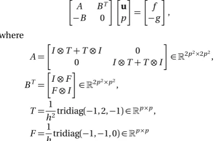
system with saddle point form (1),

A BT

−B 0

u p

=

f −g

,

where

A₌

I⊗T+T⊗I 0

0 I⊗T+T⊗I

∈R2p2×2p2,

BT=

I⊗F F⊗I

∈R2p2×p2, T= 1

h2tridiag(−1, 2,−1)∈R

p×p_, F=1

htridiag(−1,−1, 0)∈R p×p

with⊗being the Kronecker product symbol andh₌_p1₊₁

the discretization meshsize, p is a positive integer, the total number of varablesis m+n =2p2₊_p2 ₌₃_p2_{; see} [13].

IAENG International Journal of Applied Mathematics, 48:2, IJAM_48_2_15

(5)

The LCRS iterative method is compare with the classic Uzawa, GSOR, GMRES when they are used as solvers for the tested example, from the point of view of the number of total iteration steps (denoted by “IT”), the elapsed CPU time in seconds (denoted by “CPU”) and the absolute error normkuk₋_u∗_k_∞_{(denoted by “ERR”), where}

uk _{is the approximate solution satisfied the terminated}

condition of iterative methods, andu∗_{is the exact solution}

of the saddle point problem. The concrete numerical results and the corresponding parameters used in iterative methods are given in Table II.

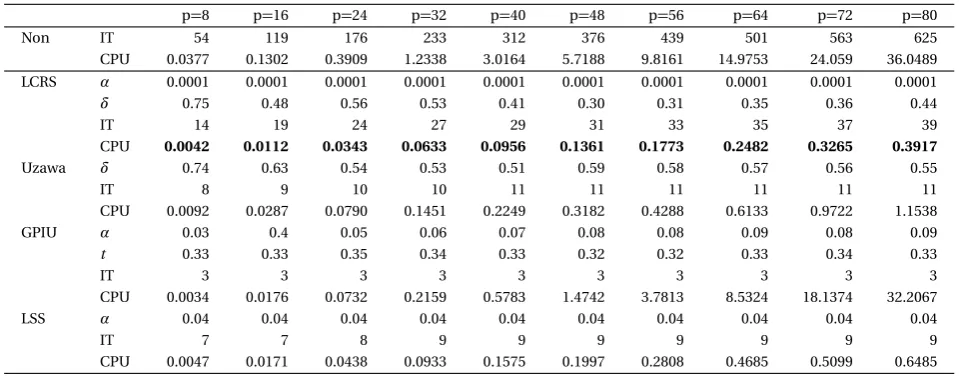
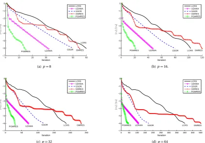
Moreover, The LCRS iteration is compare with the classic Uzawa, generalized parameterized inexact Uzawa (GPIU) and local shift-splitting (LSS) when they are used as preconditioners to accelerate GMRES for the tested problem, from the point of view of the number of total iteration steps and the elapsed CPU time in seconds, denoted by “IT” and “CPU” respectively. The empirical optimal parameters used in preconditioners and concrete numerical results are given in Table III. Furthermore, the convergence history is shown in Figure 1.

As shown in Table II and Figure 1, all iterative methods can successfully produce approximate solution of the tested saddle point problem. The elapsed CPU time and number of iterations increased as the scale of the problem increased. In terms of the number of iterations, the Uzawa iteration is the fewest, and the LCRS iterative method are fewer than GMRES but more than GSOR. In terms of the elapsed CPU time, the LCRS iteration is the least among all iterative methods.

When the LCRS is used as a preconditioner to accelerate GMRES method, from Table III, we can see that the iteration counts of GPIU preconditioner is the fewest, and those of the LCRS preconditioner is the most. But the elapsed CPU time of LCRS preconditioner is the lest. Moreover, as FFT could be paralleled and implemented on multiprocessors efficiently, the elapsed CPU time of the LCRS iterative method and the LCRS preconditioned GMRES method may be further saved.

Clearly, with the optimal parameters, the LCRS is used as either solver or preconditioner to GMRES method often do best in the elapsed CPU time, but whose iteration counts are more than Uzawa and GSOR iterative methods, also more than Uzawa, GPIU and LSS used as precondi-tioners to GMRES. This may be attributable to the follow-ing two reasons. The first is that the convergence speed of the LCRS iterative method may be slow, which directly increases the number of iterations. The other is that the FFT is used in LCRS iterative method or preconditioner, which can save a lot of time in each iteration steps. In conclusion, the LCRS is a good iterative method for solving saddle point problem (1), which is much more effective than the other tested method, and it can be used as a good preconditioner to accelerate the convergence of GMRES for the test problems.

VI. CONCLUDING REMARKS

T

HE sparse symmetric Toeplitz or BTTB structured

saddle point problems are common in many field. The local circulant and residue splitting (LCRS) iterative method and its preconditioned form are proposed to solve

the saddle point problems with the SPD Toeplitz or BTTB (1, 1)-block. In fact, the new splitting iterative method belongs to a class of the parameterized inexact Uzawa (PIU) method studied in[8], and it is also similar to the local HSS iterative method presented in[16],[27],[28]. The splitting matrix of the LCRS iterative method can serve as a preconditioner, called the LCRS preconditioner, to accelerate GMRES method for solving the saddle point problems. The main idea is the Toeplitz matrix could be split to a sum of circulant and residue matrix, and the linear sub-systems with circulant coefficient matrix could be solved by using FFT. Theoretical analysis have shown that the LCRS iterative method is feasible and effective. Numerical experiments shown that LCRS iter-ative method and the GMRES method incorporated with the LCRS preconditioner outperform other test solvers or preconditioners in elapsed CPU time.

Based on the following splitting of the saddle point matrixA:

A=

A BT

−B 0

=

G BT

−B 0

−

A−G 0

0 0

:=M−N,

whereM is called the constraint preconditioner, the main ideas in this paper could be generalized to the constraint preconditioner by further exploiting the Toeplitz structure. In [14]the convergence of the constraint preconditioned Krylov subspace iterative method was study, and it may be interesting to study the convergence of a class of splitting iterative methods based on the local circulant and residual splitting. In addition, future work should also focus on determining the choice of the optimal parameter matrices

Q1 andQ2.

ACKNOWLEDGEMENTS

The author would like to thank the anonymous referees for his/her careful reading of the manuscript.

REFERENCES

[1] Z.-Z. Bai, G. H. Golub, M. K. Ng, “Hermitian and skew-Hermitian splitting methods for non-Hermitian positive definite linear system-s”,SIAM J. Matrix Anal. Appl.vol. 24, no.3, pp. 603–626, 2003.

[2] Z.-Z. Bai, G.-Q. Li, “Restrictively preconditioned conjugate gradient methods for systems of linear equations,”IMA J. Numer. Anal.vol. 23, no. 4, pp. 561–580, 2003.

[3] Z.-Z. Bai, G. H. Golub, J.-Y. Pan, “Preconditioned Hermitian and skew-Hermitian splitting methods for non-Hermitian positive semidefinite linear systems,”Numer. Math.vol. 98, no. 1, pp. 1–32, 2004.

[4] Z.-Z. Bai, B. N. Parlett, Z.-Q. Wang, “On generalized successive overrelaxation methods for augmented linear systems,” Numer. Math., vol. 102 no. 1, pp. 1–38, 2005.

[5] Z.-Z. Bai, “Structured preconditioners for nonsingular matrices of block two-by-two structures,” Math. Comput., vol. 75, no. 254, pp. 791–815, 2006.

[6] Z.-Z. Bai, Z.-Q. Wang, “Restrictive preconditioners for conjugate gradient methods for symmetric positive definite linear systems,”J. Comput. Appl. Math., vol. 187, no. 2, pp. 202–226, 2006.

[7] Z.-Z. Bai, G. H. Golub, “Accelerated Hermitian and skew-Hermitian splitting iterative methods for saddle point problems,” IMA J. Numer. Anal., vol. 27, no. 1, pp. 1–23, 2007.

[8] Z.-Z. Bai, Z.-Q. Wang, “On parameterized inexact Uzawa methods for generalized saddle point problems,”Linear Algebra Appl., vol. 428, no. 11-12, pp. 2900–2932, 2008.

[9] Z.-Z. Bai, “Optimal parameters in the HSS-like methods for saddle-point problems,”Numer. Linear Algebra Appl., vol. 16, pp. 6, 447– 479, 2009.

IAENG International Journal of Applied Mathematics, 48:2, IJAM_48_2_15

(6)

[10] Z.-Z. Bai, “Block alternating splitting implicit iterative methods for saddle point problems from time-harmonic eddy current models,”

Numer. Linear Algebra Appl., vol. 19, no, 6, pp. 914–936, 2012.

[11] M. Benzi, G. H. Golub, J. Liesen, “Numerical solution of saddle point problems,”Acta Numer.vol. 14, pp. 1–137, 2005.

[12] M. Benzi, G. H. Golub, “A preconditioner for generalized saddle point problems,”SIAM J. Matrix Anal. Appl., vol. 26, no. 1, pp. 20– 41, 2005.

[13] Y. Cao, J. Du, Q. Niu, “Shift-splitting preconditioners for saddle point problems”.J. Comput. Appl. Math., vol. 272, pp. 239–250, 2014.

[14] Z.-H. Cao, “A class of constraint preconditioners for nonsymmetric saddle point matrices,”Numer. Math., vol. 103, no. 1, pp. 47–61, 2006.

[15] F. Chen, Y.-L. Jiang, “A generalization of the inexact parameterized Uzawa methods for saddle point problems,”Appl. Math. Comput., vol. 206, no. 2, pp. 765–771,2008.

[16] M.-Q. Jiang, Y. Cao, “On local Hermitian and skew-Hermitian splitting iteration methods for generalized saddle point problems,”

J. Comput. Appl. Math., vol. 231, no. 2, pp. 973–982, 2009.

[17] X.-Q. Jin,Developments and Applications of Block Toeplitz Iterative Solvers, Science Press, Beijing, 2006.

[18] M. K. Ng, “Circulant and skew-Circulant splitting methods for Toeplitz systems,”J. Comput. Appl. Math., vol. 159, pp. 101–108, 2003.

[19] S. Noschese, L. Reichel, “A note on superoptimal generalized Cir-culant preconditioners,”Appl. Numer. Math., vol. 75, pp. 188–195, 2014.

[20] S. Noschese, L. Reichel, “Generalized circulant Strang-type

precon-ditioners,” Numer. Linear Algebra Appl., vol. 19, no. 1, pp. 3–17, 2012.

[21] M. U. Rehman, C. Vuik, G. Segal, “Preconditioners for the Steady Incompressible Navier-Stokes Problem,”IAENG Inter. J. Appl. Math., vol. 38, no. 4, pp. 223-232, 2008.

[22] Y. Saad,Iterative Methods for Sparse Linear Systems (second ed.), SIAM, Philadelphia, 2003.

[23] J.-F. Yin, Z.-Z. Bai, “The restrictively preconditioned conjugate gradient methods on normal residual for block two-by-two linear systems,”J. Comput. Math., vol. 26, no. 2, pp. 240–249, 2008.

[24] J. H. Yun, “Performance analysis of a special GPIU method for singular saddle point problems,” IAENG Inter. J. Appl. Math., vol. 47, no. 3, pp. 325-331, 2017.

[25] Y.-Y. Zhou, G.-F. Zhang, “A generalization of parameterized inexact Uzawa method for generalized saddle point problems,”Appl. Math. Comput., vol. 215, no. 2, pp. 599–607, 2009.

[26] M.-Z. Zhu, G.-F. Zhang, “On CSCS-based iterative methods for Toeplitz system of weakly nonlinear equations,”J. Comput. Appl. Math., vol. 235, pp. 5095–5104, 2011.

[27] M.-Z. Zhu, “A generalization of the local Hermitian and skew-Hermitian splitting iterative methods for the non-skew-Hermitian saddle point problems,”Appl. Math. Comput.vol. 218, no. 17, pp. 8816– 8824, 2012.

[image:6.595.56.538.355.552.2]

[28] M.-Z. Zhu, G.-F. Zhang, Z.-Z. Liang, “On generalized local Hermitian and skew-Hermitian splitting iterative method for block two-by-two linear systems,”Appl. Math. Comput., vol. 250, pp. 463–478, 2015.

TABLE II: Numerical results of iterative methods.

p=8 p=16 p=24 p=32 p=40 p=48 p=56 p=64 p=72 p=80

LCRS α 0.26 0.21 0.20 0.20 0.20 0.20 0.19 0.19 0.19 0.19

δ 1.28 1.03 1.06 1.13 1.13 1.12 1.12 1.08 1.09 1.08

IT 59 102 158 187 242 296 359 401 459 516

CPU 0.0029 0.0068 0.0195 0.0304 0.0525 0.1000 0.1743 0.2598 0.3334 0.5389

ERR 7.90E-5 1.26E-4 1.54E-4 2.87E-4 2.94E-4 7.07E-4 5.62E-4 8.25E-4 7.29E-4 7.39E-4

Uzawa δ 0.55 0.53 0.52 0.51 0.51 0.5 0.5 0.5 0.5 0.5

IT 31 46 59 70 80 91 99 107 115 122

CPU 0.0204 0.0282 0.0667 0.1291 0.2629 0.5683 0.7189 1.286 2.3341 2.9978 ERR 6.41E-5 2.53E-4 5.05E-4 8.25E-4 1.33E-3 1.49E-3 2.16E-3 2.85E-3 3.55E-3 4.42E-3

GSOR ω 1.2 1.23 1.22 1.23 1.23 1.23 1.23 1.23 1.23 1.23

τ 0.87 0.87 0.91 0.91 0.92 0.93 0.93 0.93 0.94 0.94

IT 49 79 98 118 134 148 161 173 184 193

GMRES IT 54 119 176 233 312 376 439 501 563 625

TABLE III: Numerical results of preconditioned GMRES with different preconditioner.

p=8 p=16 p=24 p=32 p=40 p=48 p=56 p=64 p=72 p=80

Non IT 54 119 176 233 312 376 439 501 563 625

CPU 0.0377 0.1302 0.3909 1.2338 3.0164 5.7188 9.8161 14.9753 24.059 36.0489 LCRS α 0.0001 0.0001 0.0001 0.0001 0.0001 0.0001 0.0001 0.0001 0.0001 0.0001

δ 0.75 0.48 0.56 0.53 0.41 0.30 0.31 0.35 0.36 0.44

IT 14 19 24 27 29 31 33 35 37 39

CPU 0.0042 0.0112 0.0343 0.0633 0.0956 0.1361 0.1773 0.2482 0.3265 0.3917

Uzawa δ 0.74 0.63 0.54 0.53 0.51 0.59 0.58 0.57 0.56 0.55

IT 8 9 10 10 11 11 11 11 11 11

CPU 0.0092 0.0287 0.0790 0.1451 0.2249 0.3182 0.4288 0.6133 0.9722 1.1538

GPIU α 0.03 0.4 0.05 0.06 0.07 0.08 0.08 0.09 0.08 0.09

t 0.33 0.33 0.35 0.34 0.33 0.32 0.32 0.33 0.34 0.33

IT 3 3 3 3 3 3 3 3 3 3

CPU 0.0034 0.0176 0.0732 0.2159 0.5783 1.4742 3.7813 8.5324 18.1374 32.2067

LSS α 0.04 0.04 0.04 0.04 0.04 0.04 0.04 0.04 0.04 0.04

IT 7 7 8 9 9 9 9 9 9 9

CPU 0.0047 0.0171 0.0438 0.0933 0.1575 0.1997 0.2808 0.4685 0.5099 0.6485

IAENG International Journal of Applied Mathematics, 48:2, IJAM_48_2_15

[image:6.595.58.538.591.779.2]

(7)

0 10 20 30 40 50 60 −7

−6 −5 −4 −3 −2 −1 0

Iteration

k

rk

k

/

k

r0k

LCRS UZAWA GSOR GMRES PGMRES

LCRS

GSOR GMRES

UZAWA PGMRES

(a)p=8

0 20 40 60 80 100 120

−7 −6 −5 −4 −3 −2 −1 0

Iteration

k

rk

k

/

k

r0k

PGMRES UZAWA GSOR LCRS GMRES

(b)p=16.

0 50 100 150 200 250

−7 −6 −5 −4 −3 −2 −1 0

Iteration

k

rk

k

/

k

r0k

UZAWA

PGMRES GSOR LCRS GMRES

(c)p=32

0 50 100 150 200 250 300 350 400 450 500

−7 −6 −5 −4 −3 −2 −1 0

Iteration

k

rk

k

/

k

r0k

PGMRES UZAWA GSOR LCRS GMRES

[image:7.595.87.511.66.362.2]

(d)p=64

Fig. 1: Convergence of LCRS, Uzawa, GSOR, GMRES and LCRS preconditioned GMRES methods.