Full predictive cascaded speed and current control of an induction machine

Abstract—This paper presents and experimentally validates a new control scheme for electrical drive systems, named cascaded predictive speed and current control (PSCC). This new strategy uses the model predictive control concept. It has a cascaded structure like that found in field-oriented control or direct torque control. Therefore the control strategy has two loops, external and internal, both implemented with model predictive control. The external loop controls the speed, while the inner loop controls the stator currents. The inner control loop is based on Finite Control Set Model Predictive Control (FCS-MPC), and the external loop uses MPC deadbeat, making full use of the inner loop‘s highly dynamic response. Experimental results show that the proposed strategy has a performance that is comparable to the classical control strategies but that it is overshoot-free and provides a better time response.

Index Terms—Model Predictive Control, electric machines, variable speed drives, Kalman filters.

I. INTRODUCTION

Model predictive control (MPC) has undergone noteworthy growth in the last three decades [1], [2]. MPC can be used in a wide range of applications; its implementation is conceptually simple, and it exhibits very high bandwidth, a property that is exploited in this work. It is also possible, using the same framework of cost function optimization, to include control constraints and model nonlinearities [3].

Due to the large computational burden of the method and the low computation capability of early processors, MPC was initially used only in low dynamic applications with large sam-pling periods. More recently, with advanced microprocessor technology, MPC has been applied in processes with high dynamic responses. MPC applied to power electronics has two main variants: Continuous Control Set MPC (CCS-MPC) [4], [5] and Finite Control Set MPC (FCS-MPC) [6]. The CCS-MPC calculation utilizes the solution of an optimization problem, and a modulation stage generates the switching state of the converter actuation. FCS-MPC uses the discrete nature of the power converter and a model of the load to solve the optimization problem exhaustively. FCS-MPC has been used in several applications, such as conventional three-phase two-level converters [7], as well as in more complicated topologies such as multilevel converters [8], matrix converters [9] and

C. Garcia, C. Silva and C. Rojas are with the Department of Electronics Engineering, Universidad Tecnica Federico Santa Maria, Valparaiso 2390123, Chile (e-mail: [email protected]).

J. Rodriguez is with Universidad Nacional Andres Bello, Santiago, Chile. P. Zanchetta is with the Department of Electrical and Electronic Engineer-ing, University of Nottingham, Nottingham, NG7 2RD, U.K.

H. Abu-Rub is with the Department of Electrical and Computer Engineer-ing, Texas A&M University at Qatar, Qatar Foundation, Doha, Qatar.

multi-phase applications [10]. Furthermore, it has been shown that such optimal predictive current control strategies obtain faster responses and have significantly less overshoot than the well-know PI controllers [11], [12].

In a linear cascade control scheme, the bandwidth of the external speed control is limited by the dynamic response of the internal current loops. This gives rise to an explicit compromise on the bandwidth of the external loop. In [13], [14], FCS-MPC is used for the inner current and torque control of the induction machine, maximizing its dynamic response, but a classical PI controller is still used for the outer speed loop. However, by using fast current controllers, such as FCS-MPC, the response of the outer speed loop can be improved. Recently, looking to make use of the increase on performance offered by MPC, complete predictive controls of AC drives have been reported in literature, either preserving the classical cascade structure [15] or solving a single optimization problem with constraints [16], [17].

One example of an application that requires high dynamic response is servo systems [17]–[19]. A servo application in a high-performance industrial application must have a fast response, preferably without overshoot, and high steady-state accuracy. Typically, servo applications use permanent mag-netic synchronous machines, but it is also possible to find servo systems using induction machines [20].

In this paper, the cascaded structure for the control of an induction machine is revisited using the FCS-MPC inner control loops similar to those discussed in [12]–[14]. For speed control, a continuous control-set model predictive control, based on the explicit inversion of the mechanical model, is proposed. This strategy does not use a linear controller for the speed; rather, it uses a load dynamic model to calculate a reference electric torque that achieves proper tracking of the speed reference. Trusting that the inner FCS-MPC current control achieves a sufficiently fast current tracking, only the mechanical model is considered in this inversion. This is possible thanks to the high dynamic performance of FCS-MPC, the low stator transient time constant of induction machines and the use of a higher sampling rate in the inner loop. In order to invert the mechanical dynamic equation, and to achieve speed control without steady state error, the load torque needs to be included in the model. For this purpose, a Kalman filter load torque observer is proposed.

II. ANALYTICMODEL OF THEDRIVE

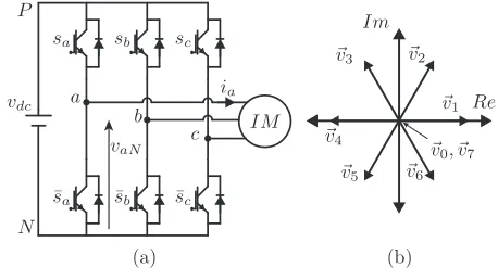
Fig. 1. Voltage vectors of 2L-VSI.

A. The Voltage Source Inverter

The two-level source inverter (2L-VSI) is a very common converter topology in drive applications due to its simplicity, its high dynamic performance and its wide availability. In a typical drive application, the converter feeds an induction machine as shown in the Fig. 1(a). Due to the nature of the converter, this topology can produce eight different voltage vectors, as illustrated in the Fig. 1(b). It is possible to identify six active voltage vectors and two zero vectors (v0andv7). The voltage vectors depend on the states of the switching converter as,

S_,2

3

Sa+ej2π/3·Sb+ej4π/3·Sc

, (1)

whereSa,Sb,Sc represent the switching state of each leg, as

shown in the Fig. 1(a). By using this notation, it is possible to write the output voltage vector in a stationaryαβ-frame as follows,

vsαβ =vdc·S, (2)

wherevdcis the dc-link voltage of the 2L-VSI shown on Fig.

1(a). To transform this voltage into a synchronous dq-frame oriented by the rotor flux, the vector rotation must be applied (3), where the θs is the rotation angle of rotor flux.

vs=vsαβe

−jθs_{. (3)}

B. Dynamic Equation of the Machine

A squirrel-cage induction machine is used in the experi-mental verification of the method. The model is developed in a synchronous frame oriented by the rotor flux angle.

The equation (4) represents the stator equation, which relates the stator current and stator linkage flux. The rotor equation, relating the rotor current and rotor linkage flux, is given in (5).

vs=Rsis+

dΨs

dt +JωsΨs, (4)

0 =Rrir+

dΨr

dt −(ωs−ω)Ψr, (5)

where,

J=

0 −1 1 0

, (6)

Fig. 2. Scheme of Cascaded Predictive Speed Control.

andvs= [vsdvsq]T is the stator voltage vector,is= [isdisq]T

is the stator current vector,ir= [ird irq]T is the rotor current

vector,Ψs= [ψsd ψsq]T is the stator linkage flux vector, and

Ψr = [ψrd ψrq]T is the rotor linkage flux vector. Also, in

these equations Rs is the stator resistance,ωs is the angular

frequency of the reference frame, Rr is the rotor resistance

andω is the rotor speed.

The flux linkage equations that relate stator and rotor linkage fluxes with stator and rotor currents are,

Ψs=Lsis+Lmir, (7)

Ψr=Lmis+Lrir. (8)

where Lm is the mutual inductance, Ls is the stator

induc-tance, andLr is rotor inductance.

Finally, the electric torque produced by the induction ma-chine can be expressed in terms of the stator current and stator flux,

T =3

2p·|Ψs×is|, (9)

wherepis the number of pole pairs.

Manipulating the above equations, the electromagnetic be-havior of the induction machine can be presented using four state variables (x = [isd isq ψrd ψrq]T), two input (u =

[vsd vsq]T) and two outputs of the system (y = [isd isq]T)

[21].

˙

x(t) =A(t)x(t) +B(t)u(t), (10)

y(t) =C(t)x(t) +D(t)u(t). (11) The matrices A, B, C and D are state-space matrices, given by

A(t) = 

   

−1

τσ ωs

kr

Rστστr

krω

Rστσ

−ωs −_τ1_σ −_Rk_σrω_{τσ Rσ}k_τr_στr Lm

τr 0 − 1

τr −(ω−ωs) 0 Lm

τr (ω−ωs) − 1

τr 

   

whereσ= 1−L2

m/(LsLr)is the total leakage factor,Rσ=

Rs+k2rRr,τσ=σLs/Rσis the transient stator time constant,

kr=Lm/Lr, andτr=Lr/Rr is the rotor time constant.

C. Discrete Model of the Machine used for Current Prediction

Firstly, it is important to consider that any digital device, typically a digital controller, operates in discrete time. For this reason, it is necessary to transform the continuous model of the system into a discrete model. Therefore, a hold device must interface between the discrete control output and the contin-uous input of the real (contincontin-uous) system. There are many options for the hold device, for example, Zero-Order Hold, First-Order Hold or the Generalized-Hold [22]. The strategy used in this work considers a Zero-Order Hold (ZOH), which simply holds the input voltage between sampling instants, i.e.,

u(t) =uk; kTs< t≤(k+ 1)Ts, (16)

whereTs is the sampling period.

If the input of the continuous-time system (10)-(11) is generated from the input sequenceuk using ZOH, then a state

space representation of the resulting sampled-data model is given by:

xk+1=Adxk+Bduk, (17)

yk =Cdxk+Dduk. (18)

The electrical sub-system is linear but has variable parameters, as can be seen in equations (10)-(15). Due to this condition, the exact discretization is not simple. Then, the matrices Ad,

Bd,Cd andDd can be obtained simply by approximating the

time derivative in (10) using the Forward Euler approximation,

s=z−1

Ts

. (19)

Finally, the discretized state-space model can be derived, leading to the following state-space matrices

Ad=I+TsA, (20)

Bd=TsB, (21)

Cd=C, (22)

Dd=D. (23)

Therefore, using the discrete dynamic equations of (17) and (18) and starting with the measured (or estimated) state values at the sampling periodkand the actuation to be applied ink, the state values ink+ 1 can be predicted.

III. THECONTROLSTRATEGY

The proposed control strategy is shown in Fig. 2. It consists of three main stages that are described in detail in this section.

A. Predictive Current Control

The control of the rotor flux is achieved only in steady state by means ofisd. An outer flux loop to achieve reference

tracking could be implemented in order to predict the flux’s dynamic performance. Such predictive flux loop would be conceptually similar to the outer speed loop to be discussed in the next subsection. However, for the sake of simplicity, this has not been implemented, as only operations below base speed are considered, i.e. no flux weakening is implemented. Therefore, there is not need to actively regulate flux.

The predictive control calculates the optimum voltage actu-ation minimizing an objective or cost function. In this case, the cost function has two simultaneous objectives, to track the quadrature stator current, i.e. tracking torque reference, and to track the direct stator current that produces the flux of the machine,

g=i∗_sq−ˆik_sq+1 2

+i∗_sd−ˆik_sd+1 2

. (24)

The cost function (24) is evaluated for each possible voltage vector of the 2L-VSI. The optimal vector that minimizes (24) is selected,

vopt= arg min

{v0,...,v7}

g(vsk+1), (25)

where, vopt is the vector of the optimum stator voltage to be

applied during the next sample time.

B. Predictive Speed Control

the inner current dynamics to be neglected for the design of the external speed loop.

dω dt =

1

J(T−TL), (26)

The inertia has been computed by using the speed slope re-sponse for an impulse quadrature stator current ofisq = 5.0[A]

operating at a nominal rotor flux ofψˆrd= 0.954[W b]and zero

load torque. Thus, the inertia can be approximated as

dω dt =

3 2J(pkr

ˆ

ψrdisq),

dω dt ≈

∆ω

∆t =

ω2−ω1 t2−t1

= 3 2J(pkr

ˆ

ψrdisq) = 570rad/s2,

J ≈ 3pLm

ˆ

ψrdisq

2Lr∆_∆ω_t

= 0.02398[Kg·m2/s], (27)

T is the electric torque and TL is the load torque.

Then, using the equation (9) and considering a synchronous

dq-frame oriented by the rotor flux, the equation (26) can be extended as follows,

dω dt = 1 J 3 2pkr

ˆ

ψrdisq−TL

. (28)

Due to the discrete nature of digital control platforms, the equation (28) must be discretized. The most common method to obtain a discrete representation of a continuous system is the Euler approximation. In particular, the Forward Euler approximation is a very simple way to discretize a continuous-time model. As discussed previously, this can be achieved by using the transformation presented in (19) to make an approximation.

1

Tds

(ωk+1−ωk) = 1

J

3 2pKr

ˆ

ψrdisq−TL

. (29)

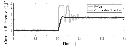
Unfortunately, the Euler approximation generates significant modeling error at high frequencies, which in turn causes problems when controlling high bandwidths [23]. As will be shown, this modeling error leads to oscillations when implementing the MPC speed control with high bandwidth. To achieve a more accurate approximation of the reference current i∗_sq, a second-order expansion for the rotor speed is proposed,

ωk+1=ωk+dω

dt _T ds

·Tds+

d2_ω dt2 _T ds ·T 2 ds

2 , (30)

where,

d2_ω dt2 =

1 J    3 2pKr

dψˆrd

dt isq+

3 2pKr

ˆ ψrd disq dt − 0 dTL dt   , (31)

and where the load torqueTLis considered invariant in a

sam-pling time. Substituting equations (28) and (31) in equation (30) and approximating the derivatives of (31) by backward Euler approximation, a closed expression for iksq is obtained.

This value for ik

sq is used as a current reference in (32)

considering i∗sq=iksq. The considerationi∗sq =iksq introduces

a delay of one sampling time Ts. However, this delay is not

1.1 1.2 1.3 1.4 1.5

0 50 100 150 Speed [rad/s] ref PI PSCC

1.65 1. 7 1.75

130 132 134 136 Speed [rad/s] ref PI PSCC 1.8 (a) (b) Time [s]

Fig. 4. Comparison between PI controller and proposed external speed loop. (a) Speed reference step; (b) Impact of load torqueTL.

Real System Process Sensor f() g() System function Measurement function Process noise Measurement noise Kalman Filter

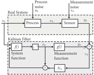
Fig. 5. Kalman filter structure.

relevant to the outer speed loop as it is implemented with a downsampling of Tds = 10·Ts. It is noteworthy that the

external loop does not introduce a significant delay because the current reference i∗sq is calculated and available for use

by the inner current control loop at the first sample timeTs

withinTds.

i∗_sq= ω

∗_−ωk₊3pKrTds 4J ·ψˆ

k rd·i

k−1

sq + Tds

J ·T k L

3pKr Tds J ˆ ψk rd− 1 4·ψˆ

k−1

rd

(32)

This quadrature stator current referencei∗_sq is used in the cost function (24). The reference generation by predictive plant inversion ideally results in reference tracking with a delay of only one sampling time (Tds), provided that the system

parameters, mainly the inertia J and the torque gain, are accurately known. Under parameter mismatch, the disturbance observer, to be discussed extensively in the next section, would help compensate for the effect of a different value of real inertia and other unmodeled mechanical effects such as friction. Nevertheless, the observer compensation is limited by its dynamic response, somewhat degrading the ideal dead-beat performance.

Fig. 3 shows a comparison of the quadrature stator current references i∗sq obtained with Euler (29) and second-order

refer-Step 4

Predict and

Evaluate for

Step 5

Calculate

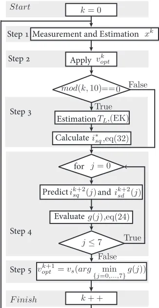
Fig. 6. Flow diagram of the complete control system.

ences, calculated with both discretization methods, are shown for a step load impact applied to the induction machine.

These results demonstrate that second-order Taylor is sig-nificantly better than the Euler discretization. Euler produces a highly oscillatory current reference, while second-order Taylor discretization of the mechanical model provides a smooth reference with only a small overshoot.

C. Kalman Filter as Load Torque Observer

To implement the proposed predictive speed controller, it is necessary to know the load torque TL, as it is required

in order to calculate the reference of the torque producing current (32). From the perspective of the loop, the load torque is an input disturbance. In the literature, there are several observers that can be used to estimate a disturbance (provided that it is observable), e.g., Model Reference Adaptive System [24], Luenberger observer [25], Kalman filter [26], Extended Kalman filter [27] or Reduce Order Kalman filter [28].

A Kalman filter is used here because it has good per-formance as a disturbance observer and at the same time it helps to obtain a filtered speed estimate from the noisy encoder position measurement. The observer estimates the load torque but also compensates for other disturbances such those produced by modeling errors. In this case, the load torque is the explicit system disturbance, but the observer also compensates for other effects of other forms that are not considered in the mechanical model, for example the friction.

for a step reference is shown; the PI controller has a greater overshoot than does the proposed external loop. The impact of the load torque is shown in Fig. 4(b); thanks to the load torque observer, the proposed method has a faster disturbance rejection than that of the PI controller.

The general structure of the filter is shown in Fig. 5. The real system with its process and measurement noise and the Kalman filter itself are the main components of the structure. The filter includes feedback of the estimation error multiplied by the Kalman gainKk.

The system considered by the filter is the mechanical dy-namics model, which is possible to represent in state variables as,

˙

x=Ex+Fu+w, (33)

y=Gx+Hu+v, (34)

where x = [ωm θm TL]T is the state vector, u = [T] is

the input, and y = [ωm] is the speed measurement. The

vector w corresponds to process noise, andv corresponds to measurement noise. The state matrixE,F,GandHare,

E=





0 0 −1

J

1 0 0 0 0 0



, (35)

F=



 1

J

0 0



, (36)

G=

1 0 0

, (37)

H= [0], (38)

where the constantJcorresponds to the inertia of the machine. It should be noted that the position is not used in the proposed algorithm, but it is considered in the system because it is easy to determine with the measurement of the speed and gives more information to the model used for the Kalman filter.

Again, the system (33)-(34) must be discretized to imple-ment the filter. It is worth highlighting that this model is linear, and therefore an exact discretization can be performed:

Ed=eETds, (39)

Fd=E−1(eETds−I)F, (40)

Gd=G, (41)

Hd=H, (42)

where Tsω is the time at which the mechanical system is

-200 -100 0 100 200

-20 0 20

0 0. 5 1 1. 5

−10 0 10

Torque [Nm]

Stator Flux [Wb]

Current [A]

Speed [rad/s]

Time [s]

0.55

0.1 0.15 0.2 0.25 0.3 0.35 0.4 0.45 0.5 0.05

(a)

(b)

(c)

(d)

Fig. 7. Experimental results of the method Full Predictive Cascaded Speed and Current Control. (a) Speed; (b) Electric Torque; (c) Stator flux; (d) stator currentia.

D. Kalman Filter Implementation

The implementation of the Kalman filter is done using equations (43)-(47). It is possible to identify two important stages, prediction and correction. The prediction estimates the state vector xk|k−1 at time k using data from the previous instant k−1 with the original linear model,

ˆ

xk|k−1=Ed·xˆk−1|k−1+Fd·uk−1, (43) Pk|k−1=Ed·Pk−1|k−1·ETd +Q. (44)

Then, the second stage, correction, estimates xk|k at time k

using the new data available in k,

Kk =Pk|k−1·GTd

h

Gd·Pk|k−1GTd +R

i−1

, (45)

ˆ

xk|k = ˆxk|k−1+Kk·(yk−Gd·xˆk|k−1), (46) Pk|k = [I−Kk·Gd]·Pk|k−1. (47) The matrix Q is the covariance of the process noise (w), and the matrix R is the covariance of the measurement noise (v). These matrices were adjusted empirically to the values given in (48) and (49). Kk is the Kalman gain, and ek is the

error between measurementykand the prediction made by the

Kalman filter.

Q=cov(w) = 



10−4 0 0 0 10−1 0 0 0 10−2



, (48) R=cov(v) =

10−6

. (49)

E. Flow diagram of the Predictive Control Strategy

This proposed strategy is represented with the flow diagram shown in Fig. 6. The steps of this flow diagram are described below:

• Step 1, the stator current, dc-link voltage and speed are measured, and the stator and rotor flux are estimated using the current model.

• Step 2, the switching state of the converter that produces the optimal voltage vector actuation, which was calcu-lated in the previous cycle, is applied.

• Step 3, when themodcondition is true (downsampled of ten sample time Ts) the predictive speed control, which

is composed of load torque estimation using the Kalman filter and the quadrature stator current (32), are estimated and calculated.

• Step 4, the response to each voltage vector of the 2L-VSI is evaluated using the cost function. The quadrature and direct stator current are predicted for the each possible voltage vector vj. Then, the predicted currents are

eval-uated in the cost function, according to (24). Finally, the cost function values (g(j)) for each voltage vector are saved for the next step.

• Step 5, the voltage vector that minimizes the cost function is selected for application in the next cycle.

strategy is coded into an algorithm in C language and imple-mented in a ds1103 dSPACE control platform. The current measurements are acquired with LEM LAH25-NP sensors, while the voltage measurements use differential amplifiers. The parameters of the induction motors are shown in Table I. To measure the speed, a quadrature incremental encoder with aresolution of 4096 ppr is used. Therefore, there is quantization noise in the position measurement in the range of −π/16384 to π/16384 radians. The control strategy uses directly the measured speed thanks to the high resolution of the encoder. In cases where the encoder may have a lower resolution, it is possible to use the filter version of the speed obtained in the Kalman filter. The inner control loop runs at a sampling time of Ts = 40[µs], while the outer speed loop

runs at a sampling time of Tsω = 400[µs]. Fig. 8 shows the

TABLE I

PARAMETERS OF THEINDUCTIONMACHINE.

Parameter Value Unit Rs 1.6647 [Ω] Rr 1.2134 [Ω] Lm 130.69 [mH]

Ls 136.81 [mH] Lr 136.81 [mH]

J 0.0239 [Kg·m2/s]

p 2

behavior of this control strategy at steady state. This result was obtained with a load torque of 10 [Nm] and at a steady speed of 90% of the rated value. Fig. 8(a) shows the phase current, which has a sinusoidal waveform without major distortion. Fig. 8(b) shows the estimated electric torque, and it is possible to observe a steady behavior with an average electric torque of 10 [Nm] that corresponds to the applied load torque. This result demonstrates the correct operation of the Kalman filter torque observer. Then, the Fig. 8(c) shows the stator flux amplitude with steady value of 0.8[Wb]. This behavior demonstrates that the stator flux is well controlled at steady state.

The stator current has a THD of 8.97%. The harmonic spectrum of the stator current and of the estimated electric torque are shown in Fig. 9. In this figure, is possible to observe the distribution of the harmonic components. This distributed behavior of the current spectrum is characteristics of FCS-MPC.

The dynamic behavior of the predictive speed control is demonstrated through a reversing speed maneuver in Fig. 7. The machine has a constant load torque of 10 [Nm] throughout the entire experiment, and then, at the time t = 0.2[s], a reversing speed reference from 90% to -90% rated speed is

0 0.01 0.02 0.03 0.04 0.05 0.06 0.07 0.08 0.09 0. 1 Time [s]

St

ato

r Flux [Wb] 0.4

Fig. 8. Steady-state operation with load torque 10 [Nm]. (a) Stator currentis, (b) electric torque and (c) stator flux.

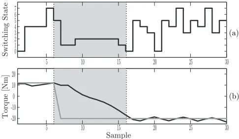
applied. The reversing maneuver is observed in Fig. 7(a). In this result, the speed does not have any appreciable overshoot when the reversing maneuver is performed. The estimated electric torque and the torque reference are shown in the Fig. 7(b). The electric torque correctly tracks the reference, and the its reference has a fast dynamics response due to the new proposed external speed loop, which has a large equivalent bandwidth. The load torque is applied by an independent load drive and its reference is kept constant during the speed reversal test. This is meant to emulate a gravitational load such that of a crane or lift in which the load torque is independent of speed. The stator flux is controlled with constant reference (0.8 [Wb]). Fig. 7(c) shows the stator flux. It is possible to observe that the stator flux is tightly controlled at all times and highly decoupled with respect to the toque. Finally, the stator current is shown in Fig. 7(d): it has a sinusoidal waveform despite the fact that its frequency and amplitude change during the acceleration and its phase changes rapidly at the beginning and end of the maneuver. The predictive speed control strategy should have a fast torque response, as shown in Fig. 10. The figure shows the behavior of the switching state before, during, and after the step in speed demand. In steady state, when the torque reference is constant, the strategy used the active and zero vectors (it should be remembered that the zero vectors are

v0andv7, as defined in section II-A). When a torque reference step is produced, due to the step in speed demand, the strategy only used the active vectors to maximize the actuation and minimize the response time. This is shown in the gray section in Fig. 10.

V. CONCLUSIONS

0 0.05 0.1

0 0.05 0.1

THD

THD

Frequency [Hz]

(a)

(b)

0 500 1000 1500 2000 2500 3000

Fig. 9. Harmonic spectrum of: (a) the stator currentisa and (b) the electric torque.

5 10 15 20 25 30

5 10 15 20 25 30

Switching State

Torque [Nm]

Sample

7 6 5 4 3 2 1 0

20 10 0 -10 -20

(a)

(b)

Fig. 10. Sequence of inverter switching state during the torque step.

end, the usefulness of an inner FCS-MPC current control has been demonstrated. With this strategy, an optimal response is obtained with a high equivalent bandwidth. Kalman filter is presented as a good alternative for estimating the load torque, which is required for the mechanical model inversion. This disturbance observer adds integration to the predictive controller and contributes to the overall system robustness. Finally, the scheme presented is validated satisfactorily with experimental results in a laboratory bench with very fast speed responses, zero steady state error and a response that is almost overshoot-free.

ACKNOWLEDGMENT

The authors acknowledge the support provided by Univer-sidad Tecnica Federico Santa Maria, by CCTVal (FB0821) and the Chilean National Fund of Scientific and Technolog-ical Development (FONDECYT) under Grants 1120683 and 1150829. Furthermore, CONICYT Scholarships supported the work of C. Garcia for PhD studies in Chile (21130140).

REFERENCES

[1] M. Morari and J. H. Lee, “Model predictive control: past, present and future,”Computers & Chemical Engineering, vol. 23, no. 4-5, pp. 667– 682, May 1999.

[2] J. Rodriguez, M. P. Kazmierkowski, J. R. Espinoza, P. Zanchetta, H. Abu-Rub, H. A. Young, and C. A. Rojas, “State of the Art of Finite Control Set Model Predictive Control in Power Electronics,”IEEE Transactions on Industrial Informatics, vol. 9, no. 2, pp. 1003–1016, May 2013.

[3] W. Xie, X. Wang, F. Wang, W. Xu, R. Kennel, and D. Gerling, “Dynamic Loss Minimization of Finite Control Set-Model Predictive Torque Control for Electric Drive System,”IEEE Transactions on Power Electronics, vol. 31, no. 1, pp. 849–860, jan 2016.

[4] A. Linder, R. Kanchan, R. Kennel, and P. Stolze,Model-Based Predictive Control of Electric Drives. Munich: Cuvillier Verlag G¨ottingen, 2010. [5] S. Mariethoz, A. Domahidi, and M. Morari, “High-Bandwidth Explicit Model Predictive Control of Electrical Drives,”IEEE Transactions on Industry Applications, vol. 48, no. 6, pp. 1980–1992, Nov. 2012. [6] P. Cortes, M. Kazmierkowski, R. Kennel, D. Quevedo, and J. Rodriguez,

“Predictive Control in Power Electronics and Drives,”IEEE Transactions on Industrial Electronics, vol. 55, no. 12, pp. 4312–4324, Dec. 2008. [7] Y. Zhang and H. Yang, “Model-predictive flux control of induction motor

drives with switching instant optimization,”Energy Conversion, IEEE Transactions on, vol. PP, no. 99, pp. 1–10, 2015.

[8] D.-K. Choi and K.-B. Lee, “Dynamic Performance Improvement of AC/DC Converter Using Model Predictive Direct Power Control With Finite Control Set,”IEEE Transactions on Industrial Electronics, vol. 62, no. 2, pp. 757–767, Feb. 2015.

[9] R. Vargas, J. Rodriguez, C. Rojas, and M. Rivera, “Predictive control of an induction machine fed by a matrix converter with increased efficiency and reduced common-mode voltage,” Energy Conversion, IEEE Transactions on, vol. 29, no. 2, pp. 473–485, June 2014. [10] H. Guzman, M. J. Duran, F. Barrero, B. Bogado, and S. Toral, “Speed

Control of Five-Phase Induction Motors With Integrated Open-Phase Fault Operation Using Model-Based Predictive Current Control Tech-niques,”IEEE Transactions on Industrial Electronics, vol. 61, no. 9, pp. 4474–4484, Sep. 2014.

[11] P. Cortes, J. Rodriguez, C. Silva, and A. Flores, “Delay Compensation in Model Predictive Current Control of a Three-Phase Inverter,”IEEE Transactions on Industrial Electronics, vol. 59, no. 2, pp. 1323–1325, Feb. 2012.

[12] C. S. Lim, E. Levi, M. Jones, N. A. Rahim, and W. P. Hew, “FCS-MPC-Based Current Control of a Five-Phase Induction Motor and its Comparison with PI-PWM Control,” IEEE Transactions on Industrial Electronics, vol. 61, no. 1, pp. 149–163, jan 2014.

[13] J. Rodriguez, J. Pontt, C. A. Silva, P. Correa, P. Lezana, P. Cortes, and U. Ammann, “Predictive Current Control of a Voltage Source Inverter,” IEEE Transactions on Industrial Electronics, vol. 54, no. 1, pp. 495–503, Feb. 2007.

[14] Y. Cho, K.-B. Lee, J.-H. Song, and Y. I. Lee, “Torque-Ripple Mini-mization and Fast Dynamic Scheme for Torque Predictive Control of Permanent-Magnet Synchronous Motors,”IEEE Transactions on Power Electronics, vol. 30, no. 4, pp. 2182–2190, Apr. 2015.

[15] Lu Gan and Liuping Wang, “Cascaded model predictive position control of induction motor with constraints,” in IECON 2013 - 39th Annual Conference of the IEEE Industrial Electronics Society. IEEE, Nov. 2013, pp. 2656–2661.

[16] E. J. Fuentes, C. A. Silva, and J. I. Yuz, “Predictive Speed Control of a Two-Mass System Driven by a Permanent Magnet Synchronous Motor,”IEEE Transactions on Industrial Electronics, vol. 59, no. 7, pp. 2840–2848, Jul. 2012.

[17] E. Fuentes, D. Kalise, J. Rodriguez, and R. M. Kennel, “Cascade-Free Predictive Speed Control for Electrical Drives,”IEEE Transactions on Industrial Electronics, vol. 61, no. 5, pp. 2176–2184, May 2014. [18] J. Holtz, M. Holtgen, and J. O. Krah, “A Space Vector Modulator for the

High-Switching Frequency Control of Three-Level SiC Inverters,”IEEE Transactions on Power Electronics, vol. 29, no. 5, pp. 2618–2626, May 2014.

[19] K. Jezernik, R. Horvat, and J. Harnik, “Finite-State Machine Motion Controller: Servo Drives,”IEEE Industrial Electronics Magazine, vol. 6, no. 3, pp. 13–23, Sep. 2012.

[20] B. Veselic, B. Perunicic-Drazenovic, and ˆA. Milosavljevic, “High-Performance Position Control of Induction Motor Using Discrete-Time Sliding-Mode Control,” IEEE Transactions on Industrial Electronics, vol. 55, no. 11, pp. 3809–3817, Nov. 2008.

[21] J. Holtz, “The dynamic representation of AC drive systems by complex signal flow graphs,” inProc. , ISIE ’94. Symp. IEEE Int Ind. Electron. Symp, 1994, pp. 1–6.

[22] J. Yuz, G. Goodwin, and H. Gamier, “Generalised hold functions for fast sampling rates,” in 2004 43rd IEEE Conference on Decision and Control (CDC) (IEEE Cat. No.04CH37601), vol. 2. IEEE, 2004, pp. 1908–1913 Vol.2.

observer,” in Applied Power Electronics Conference and Exposition, 2008. APEC 2008. Twenty-Third Annual IEEE, 2008, pp. 1796–1802. [28] E. Fuentes and R. Kennel, “Sensorless-predictive torque control of the

pmsm using a reduced order extended kalman filter,” in Sensorless Control for Electrical Drives (SLED), 2011 Symposium on, 2011, pp. 123–128.

[29] R. P. Aguilera, P. Lezana, and D. E. Quevedo, “Finite-Control-Set Model Predictive Control With Improved Steady-State Performance,” IEEE Transactions on Industrial Informatics, vol. 9, no. 2, pp. 658–667, may 2013.

[30] K. Astrom and T. Hagglund,PID controllers: theory, design, and tuning. ISA: The Instrumentation, Systems, and Automation Society; 2 Sub edition, January 1, 1995.

[31] J. Umland and M. Safiuddin, “Magnitude and symmetric optimum criterion for the design of linear control systems: what is it and how does it compare with the others?”Industry Applications, IEEE Transactions on, vol. 26, no. 3, pp. 489–497, May 1990.

Cristian Garcia (M’16) received the B.S. and M.S. degrees in electronics engineering from the Universidad Tecnica Federico Santa Maria (UTFSM),Valparaiso, Chile, in 2013. Mr. Garcia was awarded a scholarship from the Chilean Research Foundation CONICYT in 2013 to pursue his Ph.D. studies in power electronics at Universidad Tecnica Federico Santa Maria (UTFSM), Valparaiso, Chile. His research interests include matrix converters and model predictive control of power converters and drives.

Jose Rodriguez (M’81-SM’94-F’10) received the engineer degree in electrical engineering from the Universidad Tecnica Federico Santa Maria, in Val-paraiso, Chile, in 1977, and the Dr.- Ing. degree in electrical engineering from the University of Erlangen, Erlangen, Germany, in 1985. In 1977, he became a Full Professor in, and the President of the Department of Electronics Engineering, Universidad Tecnica Federico Santa Maria. Since 2015, he has been the President of the Universidad Andres Bello, Santiago, Chile. He has coauthored two books, several book chapters, and more than 400 journal and conference papers. His research interests include multilevel inverters, new converter topologies, control of power converters, and adjustable-speed drives. Dr. Rodriguez is member of the Chilean Academy of Engineering. He is the recipient of a number of best paper awards from journals of the IEEE. He was the recipient of the National Award of Applied Sciences and Technology from the Government of Chile in 2014. He was also the recipient of the Eugene Mittelmann Award from the IEEE Industrial Electronics Society in 2015.

Christian A. Rojas(S’10-M’11) was born in Val-lenar, Atacama, Chile in1984. He received the En-gineer degree in electronic enEn-gineering from the Universidad de Concepcion, Chile, in 2009, and the Ph.D. degree from the Universidad Tecnica Federico Santa Maria, Valparaiso, Chile, in 2013. Dr. Rojas was the recipient of Chilean National Research, Science and Technology Committee (CONICYT) scholarship in 2010, for his Ph.D. studies. He is cur-rently a Postdoctoral Fellow with the Solar Energy Research Center (SERC) at Universidad Tecnica Federico Santa Maria. Dr. Rojas was awarded with the Premio Tesis de Doctorado Academia Chilena de Ciencias 2012, Chile, for the best Ph.D. Thesis among of all Chilean Science Disciplines. His research interests in-clude grid-connected photovoltaic conversion systems systems, energy storage systems, advanced digital control, matrix converters, variable speed drives, model predictive control of power converters and drives.

Pericle Zanchetta (M’00-SM’15) received his de-gree in Electronic Engineering and his Ph.D. in Electrical Engineering from the Technical University of Bari (Italy) in 1994 and 1998 respectively. In 1998 he became Assistant Professor of Power Electronics at the same University. In 2001 he became lecturer in control of power electronics systems in the PEMC research group at the University of Nottingham UK, where he is now Professor in Control of Power Electronics systems. He has published over 220 peer reviewed papers; he is Chair of the IAS Industrial Power Converter Committee (IPCC) and associate editor for the IEEE transac-tions on Industry applicatransac-tions and IEEE Transaction on industrial informatics. He is member of the European Power Electronics (EPE) Executive Council. His general research interests are in the field of Power Electronics, Power Quality, Renewable energy systems and Control.