PAPER • OPEN ACCESS
Energy-efficient quantum frequency estimation
To cite this article: Pietro Liuzzo-Scorpo et al 2018 New J. Phys. 20 063009
View the article online for updates and enhancements.
Related content
Fundamental limits to frequency estimation: a comprehensive microscopic perspective
J F Haase, A Smirne, J Koodyski et al.
-Quantum-enhanced multi-parameter estimation for unitary photonic systems
Nana Liu and Hugo Cable
-Measures and applications of quantum correlations
Gerardo Adesso, Thomas R Bromley and Marco Cianciaruso
PAPER
Energy-ef
fi
cient quantum frequency estimation
Pietro Liuzzo-Scorpo1, Luis A Correa1 , Felix A Pollock2 , Agnieszka Górecka2 , Kavan Modi2 and
Gerardo Adesso1
1 School of Mathematical Sciences and Centre for the Mathematics and Theoretical Physics of Quantum Non-Equilibrium Systems, University of Nottingham, University Park, Nottingham NG7 2RD, United Kingdom
2 School of Physics and Astronomy, Monash University, Clayton, Victoria 3800, Australia E-mail:[email protected]
Keywords:quantum metrology, open quantum systems, frequency estimation, energy
Abstract
The problem of estimating the frequency of a two-level atom in a noisy environment is studied. Our
interest is to minimise
both
the energetic cost of the protocol and the statistical uncertainty of the
estimate. In particular, we prepare a probe in a
‘
GHZ-diagonal
’
state by means of a sequence of qubit
gates applied on an ensemble of
n
atoms in thermal equilibrium. Noise is introduced via a
phenomenological time-non-local quantum master equation, which gives rise to a phase-covariant
dissipative dynamics. After an interval of free evolution, the
n
-atom probe is globally measured at an
interrogation time chosen to minimise the error bars of the
fi
nal estimate. We model explicitly a
measurement scheme which becomes optimal in a suitable parameter range, and are thus able to
calculate the
total
energetic expenditure of the protocol. Interestingly, we observe that scaling up our
multipartite entangled probes offers no precision enhancement when the total available energy
is
limited. This is at stark contrast with standard frequency estimation, where larger probes
—
more
sensitive but also more
‘
expensive
’
to prepare
—
are always preferred. Replacing
by the
resource
that
places the most stringent limitation on each speci
fi
c experimental setup, would thus help to formulate
more realistic metrological prescriptions.
1. Introduction
While(classical)metrology is concerned with producing the most accurate estimate of some relevant parameter,
quantummetrology is aimed at exploiting genuinely quantum traits to go beyond classical metrological limits [1–3]. Classically, there would be no difference between running some estimation protocol sequentiallyNtimes on one probe, and running the same protocol simultaneously onn(uncorrelated)copies of that probe for
M=N/nrounds. Quantum-mechanically, however, suchn-partite probe can be prepared in an entangled state, so that itsestimation efficiencygrowssuper-extensively3. Here‘super-extensive’stands for faster-than-linear in the probe size, and the‘estimation efficiency’is proportional to the inverse of the mean squared error.
More precisely, under rather weak conditions, the statistical uncertainty of the estimate of some parameter
d
= ¯
y y ymay be tightly lower-bounded asdy1 MFy( )O [10,11], whereFy( )O denotes the Fisher
information of a sufficiently large numberMof measurements of the observableOon then-partite probe. Importantly—although often disregarded—the lengthMof the dataset used to build the estimate will always be capped by the limited availability of some essentialresource;that is, ifris the amount of resource consumed per round,M= rand hence,dy 1 h, werehºFy( )O ris the estimation efficiency. A scaling
such ash ~nc, withc>1, would be the hallmark of quantum-enhanced sensing.
Although the unavoidable effects of environmental noise often cancel out any quantum advantage[12–16], a super-extensive growth of the efficiency may still be attained under time-inhomogeneous phase-covariant noise OPEN ACCESS
RECEIVED
26 January 2018
REVISED
29 April 2018
ACCEPTED FOR PUBLICATION
17 May 2018
PUBLISHED
7 June 2018
Original content from this work may be used under the terms of theCreative Commons Attribution 3.0 licence.
Any further distribution of this work must maintain attribution to the author(s)and the title of the work, journal citation and DOI.
3Further improvements may follow from setting up interactions within the probe
[4–9], although such a scenario will not be considered in this paper.
[17–20], and even more generic Ohmic dissipation[21], noise with a particular geometry[22,23], or setups involving quantum error correction[24–26].
For instance, when it comes to frequency estimation, the total running time is usually regarded as the resource to be optimally partitioned[12]. Note that, even if features such as the amount of entanglement, coherence[27], or squeezing[28]in the initial state of the probe, or the internal interaction range among its constituents[4–7,9]could all be regarded as legitimatemetrological resources, these do notfit in our framework. That is, even if, e.g., the amount of entanglement in the preparation of ann-partite probe was severely limited in practice, this would not cap the number of roundsMof the estimation protocol—a fresh copy of thesame
entangled state would be supplied at the start of every iteration until either time, the overall number of probe constituents, or the available energy have been fully consumed.
In our case, we shall look precisely at the total energy consumed, and show that the notion ofoptimality
that follows from the maximisation of an energy efficiency differs fundamentally from the one based solely on the portioning of the available time. In particular, while the maximisation of a time efficiency encourages the use of multipartite entangled probes withnas large as possible, energetic considerations advice against it—the high
costs associated with the creation and manipulation of large multipartite correlated states does not pay off from the metrological viewpoint. In this way, we put into qualitative terms the intuitive notion that multi-particle entanglement-enabled metrology may not always be practical[29].
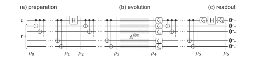
In particular, as illustrated infigure1, we consider an ensemble ofninitially thermal two-level atoms that are brought, through a sequence of qubit gates, into a sensitive GHZ-diagonal state[30](see section2.1). Such entangled probe is left to evolve freely under the action of time-non-local covariant noise. Specifically, we resort to a phenomenological quantum master equation[31–33]which explicitly accounts for memory effects and gives rise to a non-divisible dissipative dynamics[33](see section2.2for full details). We then devise a measurement protocol consisting of a sequence of qubit gates followed by an energy measurement(see section2.3). We further provide the specific measurement setting for which this scheme becomes optimal for frequency estimation in a suitable parameter range(see section2.4). By looking at the changes in the average energy of the probe during the preparation and measurement stages, we explicitly obtain the total energetic cost per round. Wefind that adjusting the free evolution time so as to maximise the time efficiency of the protocol does lead to a super-extensive scaling in the probe size; specificallyn3/2or‘Zeno scaling’[18,19]. In contrast, the energy efficiency of the very same probe, decays monotonically withn, even when the time is chosen to maximise it(see section3).
[image:3.595.122.552.64.160.2]Interestingly, note that the observed super-extensive growth of the time efficiency is attained while starting from thermal qubits that are prepared into a GHZ-diagonal state. In an accompanying article[34]the same super-extensive growth of the time efficiency is found for an arbitrary set of qubits prepared in a GHZ-diagonal state for frequency estimation in a noisy environment. The GHZ-diagonal state had been conjectured to be optimal for phase estimation with mixed probes in the absence of noise[30]. Here, we show that they lead to optimal scalingeven in a noisy scenario. We also observe that, in our setting, memoryless‘Markovian’dissipative dynamics generally produces less efficient estimates, thus suggesting that memory effects might be beneficial for the energy efficiency of parameter estimation(see section3).
Figure 1.Circuit representation of the(a)preparation,(b)free evolution, and(c)readout stages of our estimation protocol, as discussed in the main text.(a)A probe system composed of 1 control(c)qubit andn−1 register(r)qubits, initially in a thermal state
2. Methods
2.1. Probe initialisation
The system of interest is an ensemble ofnnon-interacting two-level atoms thermalised at temperatureT, whose frequencyωneeds to be estimated. For simplicity of notation we shall setÿand the Boltzmann constantkBto 1 in
all what follows. Each atom has a Hamiltonianh= w2szand is initially in the state
= 1
(
- +)
( )2
1 0
0 1 , 1
where the polarisation bias=tanh
( )
wT
2 so thatµexp(-h T), andszdenotes thezPauli matrix. The global Hamiltonian isH= w2Jz, whereJz =sz ÄÄ -n 1+ Ä sz ÄÄ -n 2++Ä -n 1Äszand the total
initial state is simply
r = º Ä =
-+
Ä Ä - Ä
Ä -⎛ ⎝ ⎜ ⎞ ⎠ ⎟ ( ) ( ) ( ) 1 2 1 0
0 1 , 2
n
c rn
n
n
0 1
1
1
where we have labelled thefirst atom ascfor‘control qubit’while the rest are taggedr, for‘register’.
We shall prepare ourn-atom probe in a GHZ-diagonal state by means of aCNOTtransformation, followed by a Hadamard gate and a furtherCNOT(seefigure1(a))[30]. That is, wefirst apply the unitary
s
ñ á Ä Ä - + ñ á Ä Ä
-∣0c 0∣c n 1 ∣1c 1∣c xn 1onr0. Introducing the denotationA¯ ºs sxA x, this yields
r =
-+ Ä Ä -⎛ ⎝ ⎜ ⎞ ⎠ ⎟ ( ) ( ) ¯ ( ) 1 2 1 0
0 1 . 3
n
n
1
1
1
Then, the Hadamard transformationUHº (sx+sz)Än -1
2
1acts solely on the control qubit:
r = - + +
-Ä - Ä
-Ä - Ä
-Ä - Ä
-Ä - Ä -⎛ ⎝ ⎜ ⎞ ⎠ ⎟ ⎛ ⎝ ⎜ ⎞ ⎠ ⎟ ¯ ¯ ¯ ¯ ( ) 1 4 1
4 , 4
n n n n n n n n 2 1 1 1 1 1 1 1 1
andfinally, the secondCNOTtransformation leads to
r = - ⎛ Ä - sÄ -Ä - + + Ä - - sÄ -Ä -⎝ ⎜ ⎞ ⎠ ⎟ ⎛ ⎝ ⎜ ⎞ ⎠ ⎟ ( ) ¯ ¯ ( ) ( ) 1 4 h.c. 1
4 h.c. , 5
n x n n n x n n 3 1 1 1 1 1 1
where the missing elements are just Hermitian conjugates of the opposite corners of each matrix. The resulting state will subsequently undergo dissipative evolution(see section2.2)before being interrogated.
As we will see in section2.2, our model of dissipation gives rise to phase-covariant dynamics. It is known that the mean squared error of frequency estimated with this type of noise can be tightly lower-boundedbelowthe standard quantum limit[19,20]. It was further shown that this bound is asymptotically saturable by using(pure) GHZ input states. On the other hand,(mixed)GHZ-diagonal states such asr3were found to perform well—and conjectured to be optimal—innoiselessphase estimation withmixedprobes[30]. In section3we will illustrate that the optimal‘Zeno scaling’, introduced in[18,19], can also be attained with such GHZ-diagonal states.
Even though in the present paper we will limit ourselves to GHZ-diagonal preparations, it seems interesting to compare the size scaling of the metrological performance ofdifferentpreparations. One would certainlyfind that some preparations may allow for a more energy-efficient estimation than othersatfixed probe size. Unfortunately, as we will see below, our calculations rely heavily on the simple analytical structure of GHZ-diagonal states undergoing phase-covariant dissipation. This makes it difficult to extrapolate our results to other initial states.
Finally, note that the energetic cost of this initialisation stageinit=tr{H(r3-r0)}is linear in the probe size and evaluates to
= 1wn ( )
2 . 6
init
At this point, one may wonder why do we not cool down probes to the ground state before starting the estimation protocol so as to work with pure rather than mixed states. This could certainly be done(e.g. by coherent feedback cooling), so long as the corresponding energy costcoolis added to the total energetic bookkeeping—just like(6),coolwould scale linearly inn. Such cooling stage is anyway not essential, and we will keep it out of the picture in what follows, thus avoiding to model it explicitly.
2.2. Free evolution
2.2.1. Phenomenological master equation
kernel[31]. The reason for this choice is that the resulting dissipative dynamics is phase-covariant, as opposed to the one following from a more canonical setting, such as the spin-boson model[21,35]. This will eventually allow us to establish a connection with known results in the literature[20]. Moreover, due to its simplicity, the model considered here can be solved exactly.
Specifically, we shall think of a generic scenario in which a two-level atom with Hamiltonianhinteracts with a bath(HB)through the interaction termHint. In the interaction picture with respect to the free Hamiltonian
= +
H0 h HB(indicated with subindexIin what follows), our phenomenological equation would read
ò
= ( - ) ( ) ( )
t sf t s s
d
d d , 7
I t
I
0
with f t( )ºle-l∣ ∣t and wheredenotes the Gorini–Kossakowski–Lindblad–Sudarshan(Markovian)
generator[36,37]
º Gw⎝⎛⎜s- s+- 1{s s+ - }+⎠⎟⎞+ G-w⎝⎛⎜s+ s-- {s s- + }+⎟⎞⎠ ( )
2 ,
1
2 , . 8
I I I I I
Here{· ·}, +stands for anti-commutator, and the decay rates areΓω≡γ0[1+(eω/T−1)−1]and
Γ−ω=e−ω/TΓω. Equation(7)comes with the advantage of explicitly introducing memory effects into the dynamics. Note, however, that one must be careful when dealing with master equations that lack a microscopic derivation[38–40]as they often lead to unphysical results. In particular, equation(7)breaks positivity ifflg 1
4
0
[32]. Importantly, the thermal sateis the stationary point equation(7), which is, in turn, consistent with our choice of initial state in section2.1.
At this point, one may still wonder why not to choose an arguably more realistic non-covariant noise model derived fromfirst principles, as in[21]. It must be noted that—unlike in[21]—we need to know the explicit form of the time-evolved state for arbitrarily large probes. This is a prerequisite for gauging the energy cost of the measurement stage, and, eventually, assessing the asymptotic scaling of the overall estimation efficiency. A noise model lacking the‘niceties’of covariant channels not only does compromise our ability to analytically evolve the state of the probe, but is also likely to render our proposed measurement scheme sub-optimal. On the plus side, however, covariant dissipation follows quite naturally from generic noise models whenever theubiquitous
rotating-wave approximation is well justified[21,35]. Furthermore, as it can be seen by comparing[20]with [34]and our results below, the details of the specific covariant dissipation model do not seem to affect the qualitative asymptotic features of the estimation protocol.
2.2.2. Connection to the damped Jaynes–Cummings model
The seemingly arbitrary choice of memory kernel in equation(7)may be justified by considering the damped Jaynes–Cummings model on resonance; that is, a two-level atom in an empty and leaky cavity. This setup can be effectively described by the Hamiltonian
å
s s s
w w
= + + +
m
m m m +
-( †) † ( )
H B B b b
2 z , 9
JC
whereBº åm mg (bm+bm†)and the system-bath coupling constantsgμmake up the Lorentzian spectral density
w = åm m d w-wm = p w-g lw +l
( ) ( ) ( )
J g2 1
2
0 2
2 2[31,35].
Assumingweak coupling, the use of a second-order Nakajima–Zwanzig master equation[35,41,42]is justified. This reads
ò
= - [H ( ) [H ( ) ( )Ä ]] ( )
t s t s s
d
d d tr , , , 10
I t
B I B
0 JC JC
where the interaction picture Hamiltonian isHJC( )t =s+( ) ( )t B t +s-( )t B†( )t , withs( )t =seiwtand = åm m m -wm + m wm
( ) ( † )
B t g b e i t bei t . The state of the environment and the trace over its degrees of freedom are
denoted byBandtrB, respectively.
Combining equations(9)and(10)one arrives to a master equation with the same structure as(7)at zero temperature[35], in which the bath correlation functionáB( )t B†( )s ñ =
ò
dw w¢J( )¢ ei(w w- ¢ -)(t s)= g le-lt2
0
plays the role of the memory kernel. In spite of this remark, we emphasise that(7)remains a purely
2.2.3. Dissipative dynamics as a phase-covariant channel
Alternatively,(7)can be brought into the Schrödinger picture and cast in the equivalenttime-localform
s s s s
s s s s s s
g g g = - + -+ - + -+ + - - + + - - + + - + ⎜ ⎟ ⎜ ⎟ ⎛ ⎝ ⎞⎠ ⎛ ⎝ ⎞⎠ [ ] ( ) { } ( ) { } ( )( ) ( ) h t t t t d
d i ,
1
2 ,
1
2 , z z z . 11
For the sake of completeness, we include here the time-dependent decay ratesγ±(t)andγz(t), derived in[33]
g( )t = - ( ) x ( ) ( )
t t
1 2 1
d
d log R and 12
g x x = ( ) ( ) ( ) ( ) t t t t 1 4 d
d log , 13
z R
R 2 2
wherexR( )t ºe-lt ⎡⎣ - sinh
(
l 1 -4R)
+cosh(
l 1-4R)
⎦⎤R
t t
2 1
1 4 2 2 and =
g l
R 0.
As argued in[20], the dissipative dynamics following from equations such as(11)can be cast a phase-covariantqubit channel( )t = L( )[ ( )]t 0 , i.e. a map such thatL ◦ j=j ◦ L, where
j ºe-ihj eihjand‘◦’stands for channel composition. These maps can be parametrised as
h w h w
h w h w
k h
L = ^ - ^
^ ^ ⎛ ⎝ ⎜ ⎜ ⎜ ⎜ ⎞ ⎠ ⎟ ⎟ ⎟ ⎟ ( ) ( )( ) ( )( ) ( ) ( ) ( ) t
t t t t
t t t t
t t
1 0 0 0
0 cos sin 0
0 sin cos 0
0 0
, 14
where the matrixL( )t acts onv( )0 =(1, tr{sx( )}0 , tr{sy( )}0 , tr{sz( )})0 to yieldv( )t = L( ) ( )t v0, so
that( )t = 12( ( )v1t +v2( )t sx+v3( )t sy+v4( )t sz).
For the ensuing dynamics to be completely positive, one must haveh( )t k( )t 1and
h h k
+ ( )t ^( )t + ( )t
1 4 2 2 . Additionally, since the map describes the action of the environment, it should asymptotically bring the two-level atom back to thermal equilibrium. This entailsk(¥ = -) [1-hz(¥)].
Following[20]one readilyfinds that equation(7)corresponds to
h k h = + + -= - -a l a l a a
- + a
a ( ) [ ( ) ] ( ) [ ( )] ( ) ( ) t
A A A
t t
e
2 e 1 1 and
1 , 15
t A
t A
1 2
whereαä{P,⊥},A= 1-4R, andA^= 1-2R.
2.2.4. State of the probe after the noisy evolution
Having discussed the details of the noise model, let us explicitly write the time-evolved stater º L[r]Än
4 3 after the action of the channel of equations(14)and(15). Its application to a generic qubit state yields
* *
a a h
h b b
L = +
+ j j - - ^ ^ -⎡ ⎣⎢ ⎤⎦⎥ ⎛ ⎝ ⎜⎜ ⎞⎠⎟⎟
( )
a c ( )c b
a b c
c a b
e
e , 16
1 1 i
i
1 1
withas º 12(1+sh+k),bsº 12(1-sh-k), andj≡ωt. As a result
r s s
a a h
b b
a a h
b b
= - L + L L
L + L
+ + L + L - L
L + L
j
j Ä
-- Ä - - ^ Ä Ä
-- Ä
-- Ä - Ä - - ^ Ä
-- Ä - Ä -⎛ ⎝ ⎜ ⎞ ⎠ ⎟ ⎛ ⎝ ⎜ ⎞ ⎠ ⎟ [ ] [ ¯ ] [ ] [ ] [ ¯ ] [ ] [ ¯ ] [ ] [ ] [ ¯ ] ( ) 1 4 e h.c. 1 4 e
h.c. , 17
n n x n n n n n x n n n 4
1 1 1 1 i 1
1 1 1 1
1 1 1 1 i 1
1 1 1 1
where we have dropped the explicit time dependence from the noise parameters for brevity. We shall not attach any energetic cost to this stage of the estimation protocol as it corresponds tofreedissipative evolution.
2.3. Probe readout
Before the probe is interrogated, it will need to undergo apre-measurementstage, consisting of sequence of three unitaries:first, each atom will be rotated by an angleζ1viazÄ1n. Then, aCNOTtransformation and the
z = =
- Ä
s s
z z z
z - ⎛ - -⎝ ⎜ ⎞ ⎠ ⎟ ( ) ( )
U e U e 1
2 1 e
e 1 , 18
H 2 i2 H i2 n
i
i
1
z z
2 2 2
2
will be sequentially applied(seefigure1(c)). An energy measurement can then be performed on the probe in order to build the frequency estimate. As we shall argue in section2.4below, in the limitR=1 , the angles(ζ1,
ζ2)may be chosen so that the statistical uncertainty of the resulting estimate is(nearly)minimal.
Let us thus obtain the probabilities associated with an energy measurement on thefinal state of the probe. The state afterzÄ -n 1
1 and theCNOTtransformation reads
r s s
s s
a a h
b b
a a h
b b
= - L + L L
L + L
+ + L + L - L
L + L
f
f Ä
-- Ä - - ^ Ä Ä
-- Ä
-- Ä - Ä - - ^ Ä
-- Ä - Ä -⎛ ⎝ ⎜⎜ ⎞⎠⎟⎟ ⎛ ⎝ ⎜⎜ ⎞⎠⎟⎟ [ ] [ ¯ ] ( [ ] ) [ ] [ ¯ ] [ ] [ ¯ ] ( [ ] ) [ ] [ ¯ ] ( ) 1 4 e h.c. 1 4 e
h.c. , 19
n n
x x n
n n
n n
x x n
n n
5
1 1 1 1 i 1
1 1 1 1
1 1 1 1 i 1
1 1 1 1
wheref≡ωt+ζ1, i.e. the action ofzÄ -1n 1amounts to replacingjj+z1in(17). It will be more convenient to castr5in an alternative form. To that end, note that
a b
L[ ]= - ∣0 0ñá ∣+ - ∣1 1ñá ∣, whereasL[ ] Ä2=
a-2 ∣00 11ñá ∣+a b- -(∣01 01ñá ∣+
b
ñá + - ñá
∣10 10∣) 2 ∣11 11∣. Generalising to an arbitrary powerlyields
å
a b L Ä = ñá
=
--
-[ ] l ( ¯ ) ( )∣x x∣, (20)
x
h x h x
l l
0 2l 1
l l
wherexlstands for thel-digit binary representation ofxandh(x)denotes the number of non-zero digits inxl(i.e.
its Hamming weight). In turn,x¯lrepresents the bitwise negation ofxl. Care must be taken not to confuse the
scalar functionh(·)with the single-atom Hamiltonianh, nor the bitwise negationx¯lwith the map¯ =s sx x.
Quantities such asL[ ¯ ] Äl,L[ ] , andL[ ¯ ] follow from equation(20)by making the replacements
- ,a- b-, anda- b, respectively, whilesxÄl∣ ¯xlñ =∣xlñ, and
s h
å
L Ä = - + j ñá
^ = -- -⎜ ⎟ ⎜ ⎟ ⎛ ⎝ ⎞⎠ ⎛⎝ ⎞⎠ [ ] ∣ ¯ ∣ ( ) ( ¯ ) ( )
[ ( ¯ ) ( )] x x
1 2
1
2 e . 21
x l l
x
h x h x
h x h x
l l 0 2 1 i l l l l l
Putting together all the above and dropping the sub-indicesl=n−1 in the interest of a lighter notation yields
å
r = f Ä ñá
f = - -- ⎛ ⎝ ⎜ ⎞ ⎠ ⎟ ∣ ∣ ( ) ( ) ( ) a c
c b x x
e
e , 22
x
x f x x
f x
x x
5 0
2 1 i
i
n 1
with the definitions
a b a b
a b a b
h
º +
º +
º - + - - +
º - +
- + - + - - + + ^ + + + ( ) ( ) [( ) ( ) ( ) ( ) ] ( ) ( ¯) ( ) ( ) ( ¯) ( ) ( ¯) ( ) ( ) ( ¯) ( ) ( ¯) ( ¯) ( ) ( ) ( ¯) a b c
f x h x h x
1
2 ,
1
2 ,
2 1 1 1 1 , and
1. 23
x h x h x h x h x
x h x h x h x h x
x n
n
h x h x h x h x
1 1
1 1
1
1 1
Similarly, thefinal state of the protocol(i.e.r6=UH( )z2 r5UH†( )z2 )is
*
å
r = z z Ä ñá
= - -- ⎛ ⎝ ⎜ ⎞ ⎠ ⎟ ˜ ˜ ˜ ˜ ∣ ∣ ( ) a c
c b x x
e
e , 24
x
x x
x x
6 0
2 1 i
i n 1 2 2 where z f z f z f
º + +
-º + -
-º - -
-˜ [ ( ( ) )]
˜ [ ( ( ) )]
˜ [ ( ( ) )] ( )
a a b c f x
b a b c f x
c a b ic f x
1
2 2 cos ,
1
2 2 cos , and
1
2 2 sin . 25
x x x x
x x x x
x x x x
2
2
2
r
r
z w z
z w z
= á ñ = + + - +
= á ñ = + - - +
∣ ∣ [ [ ( )( )]]
∣ ∣ [ [ ( )( )]] ( )
( )
( )
p x x a b c f x t
p x x a b c f x t
0, 0, 1
2 2 cos and
1, 1, 1
2 2 cos , 26
h x x x x
h x x x x
0, 6 2 1
1, 6 2 1
where all eigenvectors with the same number of 1s(i.e.h(x))on the register yield the same probability. Equation(26)will be used below to obtain a saturable lower bound on the mean squared error of the resulting frequency estimate.
We now look into the energetic cost of the pre-measurement stagemeas=( )r6 -( )r4 . Let us re-write the system Hamiltonian in the same notation as equations(22)and(24). That is,
å
w= - - - ñá + - + ñá
=
-[( ( ) ( ¯) )∣ ∣ ( ( ) ( ¯) )∣ ∣] ( )
H h x h x x x h x h x x x
2 x 1 0, 0, 1 1, 1, . 27
n
0 1
Hence,( )r4 ºtr{Hr4}writes as
r = -w
å
- - + - + = w k=
-( ) [( ( )h x h x( ¯) )a ( ( ¯)h x h x( ) )b ] n ( )
2 x 1 x 1 x 2 , 28
4
0 2n 1 1
whereas
å
å
r r wh k w z w z
= = - - + - + = - + + - - + = -= - ⎜ ⎟ ⎛ ⎝ ⎞ ⎠ ( ) { } [( ( ) ( ¯) ) ˜ ( ( ) ( ¯) ) ˜ ] ( )( ) [ ( )] ( )
H h x h x a h x h x b
n n
m c f t
tr 1 1
2 1
1
cos , 29
x x x m n m m 6 6 0 2 1
2 2 2
0 1
2 1
n 1
where the sub-indicesmindicate the Hamming weightm=h(x)of the argumentxof the corresponding coefficients, i.e.cxandfx. At our optimal prescription(ζ1,ζ2)the pre-measurement energetic cost is always
positivemeas>0.
Note that we are deliberately leaving the projective part of the measurement out of our energetic bookkeeping. In some setups such as nuclear magnetic resonance, this could be justified, as projective measurements are mimicked by suitable rotations followed by free decay. In other cases it may be necessary to supplementmeaswith a‘projection cost’proj. Similarly, depending on the specific projection model, thesharp probabilities in equation(26)might need to be modified—a‘measurement apparatus’at somefinite
temperature would arguably introduce thermally distributed random bitflips during the readout, thus making the measurementnoisy. Neither the potential extra cost nor the errors in the interrogation would qualitatively affect our results.
While very general models of projective measurement schemes, and thermodynamic analyses thereof, may be found in the literature(see e.g.[43–49], just to mention some), it is not our intention to make generic statements about the energy efficiency of frequency estimation. Instead, we settle for showing how looking at the energetic aspect of parameter estimation in a specific example can in fact change dramatically the usual notions of metrological optimality.
2.4.‘Error bars’of the estimate 2.4.1. (Classical) Fisher information
Recall from section1that the mean squared error of a frequency estimatew=w¯ dwconstructed from a sufficiently large number of measurementsMof some generic observableO, can be tightly lower-bounded as
F
dw 1 M w( )O [50], whereFw( )O stands for the(classical)Fisher information. In our case,Fw( )H can be readily computed from the probability distribution of an energy measurement onr6(see equation(26)); namely as
Fw =
å
¶ + ¶ =å
- ¶ + ¶w w w w
= -= -⎜ ⎟ ⎡ ⎣ ⎢ ⎢ ⎤ ⎦ ⎥ ⎥ ⎛ ⎝ ⎞⎠ ⎡ ⎣ ⎢ ⎢ ⎤ ⎦ ⎥ ⎥ ( ) ( ( )) ( ) ( ) ( ) ( ) ( ) ( ) ( ) H p p p p n m p p p p 1 . 30 x h x h x h x
h x m
n m m m m 0 2 1 0, 2 0, 1, 2 1, 0 1 0, 2 0, 1, 2 1, n 1
When evaluating these derivatives, one must bear in mind thatR=lg0
does depend onω, as=tanh
( )
wT
2 . However, in our modelFw( )H may be well approximated by takingRandòas constants, in the limitRλ=1 . That is,
F
å
z z wz z w
- + - + - + + - + - + w = - ⎜⎛ ⎟ ⎝ ⎞⎠ ( ) ( ) ( ) [ ( )( )] ( ) [ ( )( )] ( ) H n m
a b c n m t m n t
a b c m n t
1 4 2 sin 2
4 cos 2 . 31
m n
m m m
m m m
0
1 2 2 2 2
2 1
2 2 2
2 1
For evenn, the measurement setting(z z1, 2)=(p -w¯t, p)
2 2 maximisesFw( )H , while for oddn, one needs to choose(z z1, 2)=(p -w¯t, 0)
estimate of the atomic frequency at any given stage. As the knowledge aboutωis refined, the value ofw¯should be updated, and the measurement setting, adaptively modified. Although it may seem counter-intuitive,undoing
the precessionwÄtnon all atoms after the free evolution, improves the sensitivity to smallfluctuations ofω
around its averagew¯ and thus, helps to reduceδω.
2.4.2. Optimality of the measurement scheme
We now answer the question of whether another observableO¹Hmay give a better frequency estimate by comparingFw( )H with the quantum Fisher information(QFI)Fw=supOFw( )O [51,52]. This can be computed from the stater4right after the free evolution stage or, equivalently, fromr5, asFωis invariant under unitary transformations. The QFI is[53]
å
n rn n
=
+ áX ¶ X ñ
w w
¢= ¢
¢
( ) ∣ ∣ ∣ ∣ ( )
F 4 , 32
s s
x s
x s
x
s x
s
x s
, 2
5 2
wherenxand∣X ñx are the eigenvalues and eigenvectors ofr5. Specifically, these are
n = + D
X ñ = - D ñ + ñ
+ - D Ä ñ
w
( )
∣ ( )∣ ∣
( )
∣ ( )
( )
a b
a b c
c a b
x
1
2 and
0 2 e 1
4
, 33
x x x x
x
x x x x tf x
x x x x
i
2 2
whereD ºx (ax-bx)2+4cx2. Once again, we place ourselves in the limit of smallRλ, andfind that
r
áX ¶x∣ w 5∣X ñ =x 0, and thus
å
- -+w =
- ⎜⎛ ⎟
⎝ ⎞ ⎠
( )
( )
F n
m
n m t c
a b
1 4 2
, 34
m n
m
m m
0
1 2 2 2
which exactly coincides with the maximum of equation(31). Therefore, our proposed measurement setting is indeed optimal forRλ=1 . For arbitraryRλ, however,Fωcan be significantly larger than its limiting value(34). It may even be impossible tofind a pair(ζ1,ζ2)so thatFw( )H =Fw. Nevertheless, the exactFw( )H always
coincides with(34)atz1= p -w¯t
2 andz =
p { , 0}
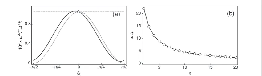
2 2 , even when this measurement setting issub-optimal. This point is illustrated infigure2(a).
3. Results and discussion
Recall that, in our scheme, the number of data pointsMthat enters the inequalitydw1 MFw( )H is limited by the available energyasM= ( init+meas). We can thus define the energy efficiency
h º
+ w
(t n, ) F . (35)
init meas
Note that we useFw( )H andFωindistinctly since, forRλ=1 , the QFI becomes saturable with our optimal measurement prescriptions.
[image:9.595.128.554.63.187.2]We will proceed to maximiseh(t n, )in two steps:first, for givenn, we shallfind the optimal interrogation timet. Then, we will look at the scaling ofh(t,n)with the probe size. From equations(6),(28),(29), and(34),
Figure 2.(a)ApproximateFw( )H for smallRλ, as in equation(31),(dashed grey curve)and exact Fisher information(solid black curve), as compared with the approximate QFI of equation(34) (dashed grey line)and the exact QFI(solid black line). The angleζ1is
set toz1=p -w¯t
2 . Note the intersection of the curves at the nearly optimal measurement settingζ2=0 .(b)Optimal interrogation timet~n-1as a function of the size of the proben. In both plotsw=w¯=1,T=200,γ0=10−4,λ=5(Rλ=0.2), andt=1.
t can be found numerically. As shown infigure2(b)it has a power-law-like dependence on the probe size
wt µn-c, wherec1(forRλ=1).
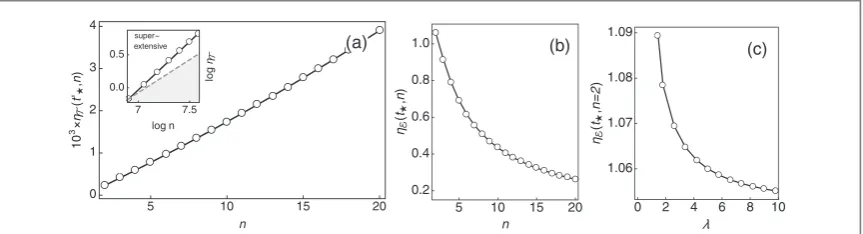
Let us place ourselves in the standard scenario, in which the total time is the scarce resource to ‘economise’on. As usual, we shall work in the limitRλ=1 and denote the corresponding optimal sampling time byt¢, respectively. Infigure3(a)we illustrate thath(t¢,n)can scale super-extensively under our
time-inhomogeneous dissipative dynamics—even if we start from(mixed)thermal probes. Specifically, we recover the Zeno scaling(δω)2∼1/n3/2[18,19].
Whatfigure3(a)suggests is that, if a large numberNof two-level atoms were available, it would be sensible to batch them together in an entangled GHZ-diagonal state and partition the available running time into prepare-and-measure segments of lengtht¢—the larger the probe, the better the resulting estimate.
In contrast,figure3(b)tells a completely different story: when adopting an entangled GHZ-diagonal preparation, the efficiencyh(t,n)decreasesrapidly as the probe is scaled up in size(in this case
h (t ,n)~n-1 3, although the exponent is non-universal). This is so because, while( + )~n init meas , the QFI exhibits a slower power-law-like growth. Hence, if there was a cap on the total available energy, one could produce a more accurate frequency estimate by manipulating the uncorrelated atomslocallyrather than attempting to build such an‘expensive’entangled state. Our numerics show that this qualitative behaviour persists even if we move away from the regime ofRλ=1 and search for the measurement setting(ζ1,ζ2)and
interrogation timetwhich jointly maximiseh(t,z z1, 2,n)=Fw( ) [H init+meas(z z1, 2)].
Another natural question to ask in this setting is whether the environmental memory time plays any role in the energy efficiency of frequency estimation. Infigure3(c)we illustrate howh(t,n)decays withλat any given
n. Recall from equation(7)that increasingλcorresponds to reducing the bath memory time, thus making the dissipation‘more Markovian’. Our setting thus showcases how memory effects in the dissipative dynamics can improve the performance of a specific parameter estimation task. Elucidating whether memory effects play an instrumental role in energy-efficient frequency estimation requires a more general analysis that we defer for future work.
4. Conclusions
We have studied the problem of noisy frequency estimation when the total available energyis limited. In each round of our estimation protocol, an ensemble ofninitially thermal two-level atoms is brought into a GHZ-diagonal form by means of a simple sequence of qubit gates. We quantified theenergetic costof the preparation stageinitby looking at the ensuing increase in the average energy of the probe.
The system is then allowed to evolve freely under the effect of environmental noise. This is modelled by a phenomenological master equation with built-in memory effects, which gives rise to phase-covariant free dissipative dynamics.
After further qubit operations, an energy measurement is eventually performed on the probe. We showed that, in a suitable range of parameters, these operations can be chosen so as to globally minimise the statistical uncertainty of thefinal frequency estimate. We also provided the corresponding optimal measurement
[image:10.595.122.554.62.179.2]prescription explicitly. The cost associated with the(pre-)measurement stagemeascan also be readily calculated from the change in the average energy of the probe, thus allowing for a comprehensive energetic bookkeeping in each round of the protocol.
Figure 3.(a)Efficiencyh(t¢,n)=F tw ¢at the optimal interrogation timet¢as a function of the probe sizen, in the standard
frequency estimation scenario of limited time. Note from the inset that, in spite of the fact that the probe is prepared in amixed GHZ-diagonal state, the efficiency grows super-extensively, ash˜ (t,n)~n3 2, which corresponds to Zeno scaling.(b)Energy
efficiencyh(t,n)=Fw (init+meas)at the optimal interrogation timetas a function of the probe sizenfor the same parameters
as(a). In this case, one roughly hash(t,n)~n-1 3, i.e. from an energetic perspective, using large entangled probes yields no
metrological advantage. In(c), we setn=2 and investigate howhattdecays asλgrows; that is, in our model, longer memory
We introduced the notion of energy efficiency of the estimationh =Fw( ) (H init+meas)as a means to assess the overall performance of the estimation protocol when there is a cap on the total energy. We further found the optimal free evolution timetmaximisingh(t,n), and noticed that preparing larger probes in
entangled GHZ-diagonal states isalways detrimentalfor the energy efficiency of frequency estimation.
In the standard scenario, one assumes that the most restrictive constraint is instead the limited running time of the estimation protocol and resorts to thefigure of merith =Fw( )H t. This grows monotonically with
nwhen optimised over the free evolution time of the probe, thus suggesting that large multipartite entangled probes are, in principle, better. This is so because afigure of merit likeh fails to capture how‘difficult’or ‘costly’it may be to prepare those states in practice. Incorporating the energetic dimension to the performance assessment through ourhmay be the simplest way to quantitatively account for this‘difficultness’.
It is true that tracking the average energy changes of the probe may be a crude way of capturing the actual limitations in force in real metrological setups. Likewise, in many situations, the total time might indeed place the most stringent limitation on the achievable precision, thus rendering other considerations irrelevant. Our observation merely highlights the importance of formulating quantifiers of the metrological efficiency that faithfully captureallthe relevant constraints in place in each specific scenario.
We also showed that, at any probe size,h(t,n)decays monotonically with the inverse bath memory time
λ, hence suggesting that large bath correlation times might be a resource for energy-efficient frequency estimation. This point certainly deserves a deeper and more general investigation.
Our intended take-home message is thatdifferent assessments of resources lead to different notions of optimality. Hence, in order to produce practically useful metrological bounds, the stress should be placed on searching for thosefigures of merit capable of capturing the most stringent limitations at work in each experimental setup.
To conclude, it is important to remark that we did not optimise our energy efficiency over the initial state of the probe but rather, adopted the GHZ-diagonal preparation as a working assumption. The question of whether or not other forms of multipartite sharing of correlations could give rise to a more energetically favourable scaling remains open and certainly deserves further investigation.
Acknowledgments
We are thankful to A del Campo, K V Hovhannisyan, J Kołodyński, R Kosloff, K Macieszczak, M Mehboudi, J Oppenheim, R Nichols, N A Rodriguez-Briones, A Smirne, T Tufarelli, and R Uzdin for helpful comments. We gratefully acknowledge funding from the Royal Society under the International Exchanges Programme(Grant No.IE150570), the European Research Council under the StG GQCOP(Grant No.637352), the Foundational Questions Institute(fqxi.org)under the Physics of the Observer Programme(Grant No.FQXi-RFP-1601), and the COST Action MP1209:‘Thermodynamics in the quantum regime’.
ORCID iDs
Luis A Correa https://orcid.org/0000-0002-7357-1328 Felix A Pollock https://orcid.org/0000-0002-1483-5661 Agnieszka Górecka https://orcid.org/0000-0003-1596-7356 Kavan Modi https://orcid.org/0000-0002-2054-9901 Gerardo Adesso https://orcid.org/0000-0001-7136-3755
References
[1]Giovannetti V, Lloyd S and Maccone L 2004Science3061330–6 [2]Giovannetti V, Lloyd S and Maccone L 2006Phys. Rev. Lett.96010401 [3]Giovannetti V, Lloyd S and Maccone L 2011Nat. Photon.5222–9 [4]Luis A 2004Phys. Lett.A3298–13
[5]Boixo S, Flammia S T, Caves C M and Geremia J 2007Phys. Rev. Lett.98090401 [6]Choi S and Sundaram B 2008Phys. Rev.A77053613
[7]Napolitano M, Koschorreck M, Dubost B, Behbood N, Sewell R and Mitchell M W 2011Nature471486–9 [8]Mehboudi M, Correa L A and Sanpera A 2016Phys. Rev.A94042121
[9]Beau M and del Campo A 2017Phys. Rev. Lett.119010403
[10]Cramér H 1999Mathematical Methods of Statisticsvol 9(Princeton, NJ: Princeton University Press) [11]Braunstein S L and Caves C M 1994Phys. Rev. Lett.723439–43
[12]Huelga S F, Macchiavello C, Pellizzari T, Ekert A K, Plenio M B and Cirac J I 1997Phys. Rev. Lett.793865–8 [13]Escher B, de Matos Filho R and Davidovich L 2011Nat. Phys.7406–11
[16]Sekatski P, Skotiniotis M, Kołodyński J and Dür W 2017Quantum127 [17]Matsuzaki Y, Benjamin S C and Fitzsimons J 2011Phys. Rev.A84012103 [18]Chin A W, Huelga S F and Plenio M B 2012Phys. Rev. Lett.109233601 [19]Macieszczak K 2015Phys. Rev.A92010102
[20]Smirne A, Kołodyński J, Huelga S F and Demkowicz-Dobrzański R 2016Phys. Rev. Lett.116120801 [21]Haase J F, Smirne A, Kołodyński J, Demkowicz-Dobrzański R and Huelga S F 2018New J. Phys.20053009 [22]Chaves R, Brask J B, Markiewicz M, Kołodyński J and Acín A 2013Phys. Rev. Lett.111120401
[23]Brask J B, Chaves R and Kołodyński J 2015Phys. Rev.X5031010
[24]Kessler E M, Lovchinsky I, Sushkov A O and Lukin M D 2014Phys. Rev. Lett.112150802 [25]Dür W, Skotiniotis M, Fröwis F and Kraus B 2014Phys. Rev. Lett.112080801
[26]Unden Tet al2016Phys. Rev. Lett.116230502 [27]Maccone L 2013Phys. Rev.A88042109 [28]Aasi Jet al2013Nat. Photon.7613–9
[29]Braun D, Adesso G, Benatti F, Floreanini R, Marzolino U, Mitchell M W and Pirandola S 2017 arXiv:1701.05152 [30]Modi K, Cable H, Williamson M and Vedral V 2011Phys. Rev.X1021022
[31]Maniscalco S and Petruccione F 2006Phys. Rev.A73012111 [32]Maniscalco S 2007Phys. Rev.A75062103
[33]Mazzola L, Laine E M, Breuer H P, Maniscalco S and Piilo J 2010Phys. Rev.A81062120
[34]Górecka A, Pollock F A, Liuzzo-Scorpo P, Nichols R, Adesso G and Modi K 2017 arXiv:quant-phys/1712.08142 [35]Breuer H and Petruccione F 2002The Theory of Open Quantum Systems(New York: Oxford University Press) [36]Lindblad G 1976Commun. Math. Phys.48119–30
[37]Gorini V, Kossakowski A and Sudarshan E 1976J. Math. Phys.17821 [38]Levy A and Kosloff R 2014Europhys. Lett.10720004
[39]Barnett S M and Stenholm S 2001Phys. Rev.A64033808 [40]Stockburger J T and Motz T 2016Fortschr. Phys.656–8 [41]Nakajima S 1958Prog. Theor. Phys.20948–59 [42]Zwanzig R 1960J. Chem. Phys.331338–41
[43]Sagawa T and Ueda M 2009Phys. Rev. Lett.102250602 [44]Erez N 2012Phys. Scr.2012014028
[45]Jacobs K 2012Phys. Rev.E86040106
[46]Micadei K, Serra R M and Céleri L C 2013Phys. Rev.E88062123 [47]Faist P, Dupuis F, Oppenheim J and Renner R 2015Nat. Commun.67669 [48]Abdelkhalek K, Nakata Y and Reeb D 2016 arXiv:quant-phys/1609.06981 [49]Kammerlander P and Anders J 2016Sci. Rep.622174
[50]Barndorff-Nielsen O and Gill R 2000J. Phys. A: Math. Gen.334481 [51]Paris M G 2009Int. J. Quantum Inf.7125–37
[52]Kołodyński J 2014 arXiv:quant-phys/1409.0535