Introduction to Cartesian, Tensor and Lexicographic Product of Bipolar Interval Valued Fuzzy Graph

(1)

ISSN: 1816-949X

Introduction to Cartesian, Tensor and Lexicographic Product of

Bipolar Interval Valued Fuzzy Graph

1

_{Wael Ahmad Al Zoubi,}

2

_{As’ad Mahmoud As’ad Alnaser,}

3

_{Hazem “Moh’d Said” Hatamleh,}

4

_{Youssef Al Wadi and}

5

_{Mourad Oqla Massa’deh}

1, 2, 3, 5

_{Department of Applied Science, Ajloun University College, Al-Balqa Applied University,}

Salt, Jordan

3

Department of Computer, Science College, Taibah University, Medina, Saudi Arabia

4

Department of Mathematics, Arab International University, Dara, Syria

5

Department of Mathematics, Faculty of Science, Taibah University, Medina, Saudi Arabia

Abstract: In this study, we discuss the product of bipolar, interval valued fuzzy graphs concept and we give some properties for them. We will study some corollaries on Cartesian product and define some properties on it. Tensor product, lexicographic product of bipolar interval valued fuzzy graph will also be defined.

Key words: Interval valued fuzzy set, bipolar interval valued fuzzy set, bipolar interval valued fuzzy graph,

cartesian product, tensor product, lexicographic product

INTRODUCTION

A fuzzy set theory was introduced by Zadeh (1965). Fuzzy set theory has become a vigorous area of research in different disciplines including mathematics, physics, statistics, engineering and computer networks. In mathematics fuzzy groups, rings and graphs have been discussed by Massa’deh (2010a, b), Massa’deh and Ba’arah (2013) and Massa’deh and Gharaibeh (2011). Bipolar fuzzy set’s concepts defined by Zhang (1998) is a generalization of fuzzy sets (Muthuraj et al., 2016; Muthuraj and Sridharan, 2012) discussed the concepts of bipolar fuzzy normal-subgraph (Massa’deh, 2017) introduced and studied bipolar fuzzy cosets. Ramya and Lavanya (2017) studied the edge contraction on bipolar fuzzy graphs (Massa’deh and Ba’arah, 2013) introduced the concept of degrees types in bipolar fuzzy graphs. Akram and Dudek (2011) extended the fuzzy set theory to interval-valued fuzzy sets, in addition (Ramprasad et al., 2016) discussed interval valued fuzzy graphs, also (Massa’deh, 2017) discussed regular, degree of vertex, strong, complete interval valued fuzzy graphs (Rashmanlou and Pal, 2013a-c; Rashmanlou and Jun, 2013). Mishra et al. studied bipolar interval valued fuzzy graphs (Mishra and Pal, 2016). In this study, we gave and studied the product of two bipolar interval-valued fuzzy graph concepts and discussed some of their properties, we defined also tensor product and lexicographic of bipolar interval-valued fuzzy graphs.

MATERIALS AND METHODS

Preliminaries

Definition 2.1 (Zadeh 1965): A fuzzy set μ is a mapping

from X to [0, 1].

Definition 2.2 (Massa’deh and Gharaibeh (2011): A

fuzzy graph G is a pair of functions G = (λ, μ) where, λ is a fuzzy subset of a non-empty set X and μ is a symmetric fuzzy relation on λ this means that μ (xy)#max {λ (x), λ (y)}. The underlying crisp graph of G = (λ, μ) is denoted by G* = (V, E) where EfV X V.

Definition 2.3 (Massa’deh and Ba’arah (2013): Let

G = (λ, μ) be a fuzzy graph, the degree of a vertex a0G is defined by:

 

G

D a =



a b ab =



ab E ab

Definition 2.4 (Massa’deh and Ba’arah (2013): The

order of a fuzzy graph G is defined by O (G) = Gab0Eλ (a):

Definition 2.5 Zhang (1998): Let X be a non-empty set.

A bipolar fuzzy set μ in X is an object having the form μ = {(x, μ+_(x),_μ_G_{(x)); x}₀_{X} where}_μ+_{(x): X}₆_{[0, 1] and}_μ_G

(x): X6[-1, 0] are mapping. Here, μ+_{(x) is the positive}

membership value which denotes the satisfaction degree of an element x0μ and μG(x) is the negative membership value which denotes the satisfaction degree to some implicit counter property of an element x0μ. If for any

(2)

x0μ, μ+_(x)_…_{0 and}_μ_G_{(x) = 0, it is the situation that x has}

only positive satisfaction for μ, if for any x0μ, μ+_{(x) = 0}

and μG(x)…0 then the situation that x does not satisfy the property of μ but somewhat satisfies the counter property of μ. It is possible for an element x for which μ+

(x) = 0 and μG(x) = 0 then we say that the satisfaction property of an element overlaps with its counter satisfaction property over some portion, we shall use the symbol μ (μ+_,_μ_G_{) for the bipolar fuzzy set}_μ_{= {(x,}_μ+_(x),

μG (x)); x0μ}.

Definition 2.6 (Zhang, 1998): For every two

bipolar fuzzy sets μ = (μ+_,_μ_G_{) and}_λ_{= (}_λ+_,_λ_G_{) in}

A, we define:



 



 





   





 



 





   



+ + -

-+ + -

-a = (min a , a , max a , a

a = (max a , a , min a , a

      

      

For all a0A:

Definition 2.7 (Zhang, 1998): Let μ = (μ+_,_μ_G_{) and}_λ₌

(λ+_,_λ_G_{) be two bipolar fuzzy sets on A. If}_δ₌_μ_×_λ_{is any}

relation on A then δ = (δ+_,_δ_G_{) is called a bipolar fuzzy}

relation from μ = (μ+_,_μ_G_{) on}_λ_{= (}_λ+_,_λ_G_{) where}_δ+_(a,

b)#min {μ+_(a),_λ+_{(b)} and}_δ_G_{(a, b)}_$_{max {}_μ_G_(a),_λ_G_(b)}

for all a0μ and b0λ.

Throughout this study, G is a crisp graph, FG is a

fuzzy graph, BFG is a bipolar fuzzy graph, IVFG is an

interval-valued fuzzy graph and BIVFG is a bipolar

interval-valued fuzzy graph.

Let A = {a1, a2, ..., an} be any set and [0, 1] be the set

of all closed sub-intervals of the interval [0, 1], [-1, 0] be the set of all closed sub-intervals of the interval [-1, 0] and elements of these sets are denoted by uppercase letters. If μ0C [0, 1] or K [-1, 0] then it can be represented as μ = [μL, μu] where μL and μu are the lower and upper

limit of μ.

Definition 2.8 (Mishra and Pal, 2016) BIVF

subset is given by μ = {<a, μ+_(a),_μ_G_{(a)>, a}₀_{A} where}

μ+_{: A}₆_{C [0, 1],}_μ_G_{: A}₆_{K [-1, 0]. The intervals}_μ+_{(a) and}

μG (a) denote the degree of membership and the degree of non-membership of the element a to the set, where μ+_{(a) = [}_μ+

L (a), μ +

U (a)] and μG (a) = [μGL

(a), μG_U (a)].

Definition 2.9 (Mishra and Pal, 2016): By bipolar

interval-valued fuzzy set on V and λ = [λG, λ+_{] is a bipolar}

interval-valued fuzzy relation on E such that: C λG (ab)#min {μG (a), μG (b)}

C λ+_(ab)_#_{min {}_μ+_(a),_μ+_{(b)} for all ab}₀_E

Definition 2.10 (Ramya and Lavanya, 2017): By a

bipolar fuzzy graph BFG of G = (V, E) we main a pair (δ,

γ) where δ = (δ+_,_δ_G_{) is a bipolar fuzzy set on V and}_γ₌

(γ+_,_γ_G_{) is a bipolar fuzzy relation on E}_f_{V X V such that}

γ+_(ab)_#_{min {}_δ+_(a),_δ+_{(b)} and}_γ_G_(ab)_#_{max {}_δ_G_(a),_δ_G

(b)} for all a, b0V and ab0E.

Definition 2.11 (Rashmanlou and Pal 2013): Let

G1 = (V1, E1) and G2 = (V2, E2) be two simple

graphs, we can construct several new graphs. The first construction called the Cartesian product of G1 and G2

gives a graph G1.G2 = (V, E) with V = V1 X V2 and E =

{(a, b) (a, c); a0V1, bc0E2} U {(d1, e) (d2, l); d1d20E1,

e0V2}.

Throughout this study, we assume C [0, 1] be the set of all closed sub-intervals of the interval [0, 1] and K [-1, 0] is the set of all closed sub-intervals of the interval [-1, 0].

RESULTS AND DISCUSSION

Definition 3.1: A Bipolar Interval-valued Fuzzy Graph

BIVFG with underlying graph G = (V, E) is defined to be

a pair (λ, μ) where:

The function λ+_{: V}₆_{C [0, 1] and}_λ_G_{: V}₆_{K [-1, 0]}

denote satisfaction degree interval and the satisfaction degree interval to some implicit counter-property of an element a0λ, respectively.

The function μ+_{: E}_d_{V X V}₆_{C [0, 1] and}_μ+_{: E}_d_{V X}

V6K [-1, 0] are defined by μ+

L (a, b)#min {λ +

L (a), λ +

L

(b)} and μGL (a, b)$max {λGL (a), λGL (b)} μ +

U (a, b)#min

{μ+ U (a), μ

+

U (b)} and μGU (a, b)$max {μGL (a), μGU (b)}

for all ab 0E.

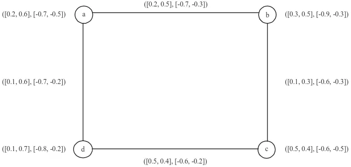
Example 3.2: Consider a Bipolar Interval-valued Fuzzy

graph BIFG where, λ = (a, [0.2, 0.6], [-0.7, -0.5]), (b, [0.3,

0.5], [-0.9, -0.3]), (c, [0.5, 0.4], [-0.6, -0.5]), (d, [0.1, 0.7], [-0.8, -0.2]). Then the corresponding BIVFG is shown in

Fig. 1.

Definition 3.3: Let G1 = (λ1, μ1) and G2 = (λ2, μ2)

be two bipolar interval valued fuzzy graph of the graph is G*

1 = (V1, E1) and G *

2 = (V2, E2) then the

Cartesian product G = (G1×G2) is defined as pain

(λ1, λ2, μ1×μ2) such that:





 



 







 



 







 



 







 



 







+ + + +

1L 2L 1L 2L

+ + + +

1U 2U 1U 2U

1L 2L 1L 2L

1U 2U 1U 2U

× a, b = min a , b

× a, b = max a , b

For all a, b V

   

   

(3)

a b

d c

([0.2, 0.6], [-0.7, -0.5])

([0.1, 0.6], [-0.7, -0.2])

([0.1, 0.7], [-0.8, -0.2])

([0.5, 0.4], [-0.6, -0.2])

[image:3.612.126.479.98.266.2]

([0.5, 0.4], [-0.6, -0.5]) ([0.1, 0.3], [-0.6, -0.3]) ([0.3, 0.5], [-0.9, -0.3]) ([0.2, 0.5], [-0.7, -0.3])

Fig. 1: Bipolar interval-valued fuzzy graph







  





 









  





 









  





 









  





 



+ + + +

1L 2L 1L 2L

+ + + +

1U 2U 1L 2U

1L 2L 1L 2L

1U 2U 1U 2U

2

× a, b a,c = min a , bc

× a, b a,c = max a , bc

For all a V and bc E

   

   

 







  





 









  





 









  





 









  





 



+ + + +

1L 2L 1L 2L

+ + + +

1U 2U 1U 2L

1L 2L 1L 2L

1U 2U 1U 2U

1

× a, b c, b = min ac , b

× a, b c, b = max ac , b

× a, b c, b = max a , b

For all b V and ac E

   

   

 

Definition 3.4: If G1 = (λ1, μ1) and G2 = (λ2, μ2) are two

bipolar interval valued fuzzy graph of G*

1 = (V1, E1) and

G*

2 = (V2, E2), respectively then the lexicographic product

G1*G2 is defined as a pair (λ, μ) where λ = (λ

+_,_λ_G_{) and}_μ

= (μ+_,_μ_G_{) are bipolar interval valued fuzzy sets on V =}

V₁×V₂ and E = {(a, b) (a, c); a0V₁, (b, c) 0 E₂} c {(x, y) (z, w); xz0E1, yw0E2}, respectively which satisfies the

following conditions:





 



 







 



 







 



 







 



 







+ + + +

1L 2L 1L 2L

+ + + +

1U 2U 1U 2U

1L 2L 1L 2L

1U 2U 1U 2U

1 2

* x, y = min x , y

* x, y = max x , y

For all x, y V ×V

   

   









  





 









  





 









  





 









  





 



+ + + +

1L 2L 1L 2L

+ + + +

1U 2U 1U 2U

1L 2L 1L 2L

1U 2U 1L 2U

1 2

* a, b a,c = min a , bc

* a, b a,c = min a , ac

* a, b a,c = max a , ac

For all a V and bc E

   

   

 







 





 









 





 









 





 









 





 



+ + + +

1L 2L 1L 2L

+ + + +

1U 2U 1U 2U

1L 2L 1L 2L

1U 2U 1U 2U

1 2

* x, y z, w = min xz , yw

* x, y z, w = max xz , yw

For all xz E and yw E

   

   

 

Definition 3.5: Let G1 = (λ1, μ1) and G2 = (λ2, μ2)

be two bipolar interval valued fuzzy graph of G* 1 = (V1,

E₁) and G*

2 = (V2, E2), respectively then the tensor

product G1qG2 is defined as a pain (λ, μ) where λ

and μ are bipolar interval valued fuzzy sets on 1 2 V = V ´V and V = V1×V2 and E = {(a, b) (c, d);

(a, c) 0E1, (b, d) 0 E2}, respectively which satisfies the

following axioms:





 



 







 



 







 



 







 



 







+ + + +

1L 2L 1L 2L

+ + + +

1U 2U 1U 2U

1L 2L 1L 2L

1U 2U 1U 2U

1 2

a, b = min a , b

a, b = max a , b

For all a, b V ×V

   

    









  





 









  





 









  





 









  





 



+ + + +

1L 2L 1L 2L

+ + + +

1U 2U 1U 2U

1L 2L 1L 2L

1U 2U 1U 2U

1 2

a, b c,d = min ac , bd

a, b c,d = max ac , bd

For all ac E and bd E

   

    

 

Definition 3.6: If G1, G2 are two bipolar interval valued

fuzzy graph and G = G₁×G₂ is the Cartesian product of G₁ and G2 then for any vertex (a, b)0V1×V2, we define the

(4)

(a)

(b)

([0.3, 0.7], [-0.6, -0.4])

([0.2, 0.5], [-0.5, -0.3])

([0.4, 0.8], [-0.7, -0.3])

([0.5, 0.3], [-0.8, -0.5])

([0.4, 0.1], [-0.7, -0.2])

([0.7, 0.2], [-0.9, -0.4])

a b

c d

[image:4.612.329.531.100.244.2]

(a, b) ([0.3, 0.6], [-0.6, -0.2]) ([0.2, 0.3], [-0.5, -0.1])

(a, c) ([0.3, 0.3], [-0.5, -0.3])

(b, d) ([0.4, 0.7], [-0.6, -0.2]) ([0.4, 0.2], [-0.6, -0.1]) (c, d) ([0.5, 0.2], [-0.8, -0.4])









  



  







  



  



 





 





 

1U 2U 1U 2U 2 1 2 1 + + + G

a ,b c,d E - -a ,b c,d E

+ +

1U 2U

a = c, bd E

+ +

2U 1U

b = d, ac E

1U 2U

a = c, bd E _2U b = d, ac E _1U

D a, b = × a, b c,d

-× a, b c,d =

min a , bd +

min b , ac

-a , b ,

max + max

bd ac                                              



Similarly:









  



  







  



  



 

2 1L L 2 L 1L 2 1 2 1 + + G

a ,b c,d E -

-a ,b c,d E

+ +

1L 2L

+ +

a = c, bd E 2L b = d, ac E _1L

1L 2L

a = c, bd E _2L b = d, ac E _1L

D a, b = × a, b c,d

-× a, b c,d =

a , b ,

min + min

-bd ab

a , b ,

max + max

bd ac                                                           



         

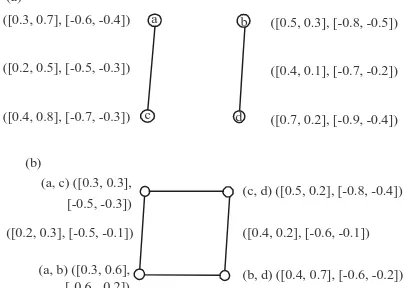
Example 3.7: Consider a bipolar interval valued fuzzy

graphs G1, G2 and G1×G2 in Fig. 2.

Definition 3.7: A Cartesian product of graph is:

C Strong, if DGG#0 and D +

G>0

C Week, if DGG<0 and D +

G$0

C Super strong, if DGG<0 and D +

G>0

C Very week, if DG_G<0 and D+ G>0

Theorem 3.8: Let G be the Cartesian product of two

bipolar interval valued fuzzy graphs then G is super strong if:

C Min {λ+

iL (ai)}$max {λGiL (ai)}

C Min {λ+

iU (ai)}$max {λGiU (ai)}

Proof SinG G is super strong if and only if DGG<0

and D+ G>0:





  















  















  















  











1 2 1 2

1 2 1 2 1L 2L

a , a b , b E

1 2 1 2 1L 2L

a , a b , b E

1 2 1 2 1L 2L

a , a b , b E

1 2 1 2 1L 2L

a , a b , b E

× a ,a b , b

-× a ,a b , b <0

× a ,a b , b <

× a ,a b , b *

                   



Fig. 2: Cartesian product of G1, G2

Now:





  















  















  















  











1 2 1 2

1 2 1 2 1L 2L

a , a b , b E

1 2 1 2 1L 2L

a , a b , b E

1 2 1 2 1L 2L

a , a b , b E

1 2 1 2 1L 2L

a , a b , b E

× a ,a b , b

-× a ,a b , b <0

× a ,a b , b <

× a ,a b , b *

                   



Such that n = number of edges and i = 1, 2, 3, ..., n by the same case we get:





1 21 2











 





1 2 1 2 iL i

1L 2L a , a b , b E

× a ,a b , b = n max a

  



  



By *, we get min {λGiL (ai)}$max {λGiL (ai)}.

Similarly, we can show {λGiU (ai)}$max {λGiU (ai)}.

Corollary 3.9: If G1, G2 are two super strong Cartesian

product graph then the Cartesian product is always super strong.

Proof: Since, G1, G2 are two super strong

Cartesian product graph then and and 1 -G D <0 1 + G D >0

and we know and

2

G

D <0

2

G

D >0 D-G ×G₁ ₂ = D-G₁+D-G₂

for the Cartesian product of bipolar

1 2 1 2

+ + + G ×G G G

D = D +D

interval valued fuzzy graph. By theorem 3.7 we get .

1 2 1 2

+ G ×G G ×G

D <0 and D >0.

Lemma 3.10: If G1, G2 are two very week Cartesian

product graph then G1×G2 is always very week.

(5)

Definition 3.11: For any vertex (a1, a2)0V1qV2 then the

degree of a vertex in tensor product is:





  











  































1 2

1 2 1 2

1 1 1 2 2 2

1

G G 1L 2L 1 2 1 2

a , a b , b E 2

1 2 1 2 1L 2L

a , a b , b E

1 1 2 2

1L 2L

a , b E , a , b E

1 1 2 2

1L 2L

a , b E , a , b E

a ,

D = a ,a b , b

-a

a ,a b , b =

min a b , a b

-max a b , a b

  





 



 

 

 

 

  _{  }

   

  

 



Definition 3.12: For any vertex (a1, a2)0V1*V2 then the

degree of a vertex in lexicographic product is:





  











  







 





 





 





1 2

1 2 1 2

1 1 2 2

2 2 2 1 1 1

G *G 1L 2L 1 2 1 2

a , a b , b E

1 2 1 2 1L 2L

a , a b , b E

+ +

1L 1 1L 2

+ +

a = b , _2L ₂ ₂ a = b , _1L _{1 1}

a b E a b E

-1L 1 -2L 2 2

D = × a ,a b , b

-× a ,a b , b =

a , a ,

max min , min

-a b a b

a ,

max max

a b

  



 



 

 

 __ _ __ _

    

    

 

   

    

 

 

   



 





1 1 2 2

2 2 2 1 1 1

-1L 2

-a = b , a = b , 1L 1 1

a b E a b E

a ,

, max

a b

 

 __ _

   

   



  

   

 



CONCLUSION

In this study, we introduce the degree and discuss it for Cartesian product, tensor product and lexicographic product of two bipolar interval valued of fuzzy graphs also we can generalized it to like strong product, week product. We use this concept in homomorphism bipolar interval valued fuzzy graph and in bipolar intuitionistic interval valued fuzzy graph on the other hand the concept of fuzzy sets, bipolar fuzzy sets and intuitionistic fuzzy sets will be applied to the following topics listed by Alnaser (2014a, b, 2017, 2018).

REFERENCES

Akram, M. and W.A. Dudek, 2011. Interval-valued fuzzy graphs. Comput. Math. Appl., 61: 289-299.

[image:5.612.95.274.271.390.2]

Alnaser, A.M., 2014b. Set-theoretic foundations of the modern relational databases: Representations of table algebras operations. Br. J. Math. Comput. Sci., 4: 3286-3293.

Alnaser, A.M., 2014a. Streaming algorithm for multi-path secure routing in mobile networks. IJCSI. Intl. J. Comput. Sci. Issues, 11: 112-114.

Alnaser, A.M., 2017. A method of forming the optimal set of disjoint path in computer networks. J. Appl. Comput. Sci. Math., 11: 9-12.

Alnaser, A.M., 2018. A method of multipath routing in SDN networks. Adv. Comput. Sci. Eng., 17: 11-17.

Massa’deh, M.O. and A. Ba’arah, 2013. Some contribution on isomorphic fuzzy graphs. Adv. Applic. Discrete Math., 11: 199-206.

Massa’deh, M.O. and N.K. Gharaibeh, 2011. Some properties on fuzzy graphs. Adv. Fuzzy Math., 6: 245-252.

Massa’deh, M.O., 2010a. A note on upper fuzzy subrings and upper fuzzy ideals. S. East Asian J. Math. Math. Sci., 9: 41-49.

Massa’deh, M.O., 2010b. Short communicationsome properties of upper fuzzy order. Afr. J. Math. Comput. Sci. Res., 3: 192-194.

Massa’deh, M.O., 2017. On bipolar fuzzy cosets, bipolar fuzzy ideals and isomorphisms of γ-near rings. Far East J. Math. Sci., 102: 731-747.

Mishra, S.N. and A. Pal, 2016. Bipolar interval valued fuzzy graphs. Intl. Sci., 9: 1022-1028.

Muthuraj, R. and M. Sridharan, 2012. Bipolar anti fuzzy HX group and its lower level sub HX groups. J. Phys. Sci., 16: 157-169.

Muthuraj, R., M. Sridharan and K.H. Manikandan, 2016. Some properties of bipolar fuzzy normal HX subgroup and its normal level sub HX groups. Global Res. Dev. J. Eng., 2: 57-65.

Ramprasad, N. Srinivasarao and S. Satyanarayana, 2016. A study on interval-valued fuzzy graphs. Comput. Sci. Telecommun., 50: 60-72.

Ramya, S. and S. Lavanya, 2017. Edge contraction on bipolar fuzzy graphs. Intl. J. Trend Res. Dev., 4: 475-477.

Rashmanlou, H. and M. Pal, 2013b. Antipodal interval valued fuzzy graphs. Intl. J. Appl. Fuzzy Sets Artif. Intell., 3: 107-130.

Rashmanlou, H. and M. Pal, 2013a. Balanced interval-valued fuzzy graphs. J. Phys. Sci., 17: 43-57.

Rashmanlou, H. and M. Pal, 2013. Some properties of highly irregular interval-valued fuzzy graphs. World Appl. Sci. J., 27: 1756-1773.

Rashmanlou, H. and Y.B. Jun, 2013. Complete interval-valued fuzzy graphs. Ann. Fuzzy Math. Inf., 6: 677-687.

Zadeh, L.A., 1965. Fuzzy sets. Inform. Control, 8: 338-353.