Munich Personal RePEc Archive
Commodity house prices
Leung, Charles Ka Yui and Shi, Song and Tang, Edward Chi
Ho
City University of Hong Kong, Massey University, Hong Kong Shue
Yan University
September 2013
Online at
https://mpra.ub.uni-muenchen.de/49489/
Commodity House Prices
Charles Ka Yui Leung, City University of Hong Kong
Song Shi, Massey University
Edward Tang, Hong Kong Shue Yan University
This version: September 2013
Abstract
This paper studies how commodity price movements have affected the local house prices in
commodity-dependent economies, Australia and New Zealand. We build a geographically
hierarchical empirical model and find the commodity prices influence local house prices directly
and also indirectly through macroeconomic variables. The impacts of commodity price changes
are analogous to “income shocks” rather than “cost shocks”. Regional heterogeneity is also
observed in terms of differential dynamic responses of local house prices to energy versus
non-energy commodity price movements. The results are robust to alternative approaches. Directions
for future research are also discussed.
JEL classification: F40, G10, R30
Keywords: regional economies, energy versus non-energy commodity price, propagation
mechanism, geographically hierarchical model, dynamic analysis
Acknowledgement: The authors are grateful to many colleagues and friends, especially Nan‐Kuang Chen, Xu Han, Dan McMillen, Peng Wang, Isabel Yan, seminar participants of the City University of Hong Kong Brown Bag, Massey University, Southwest University of Finance and Economics, Tsinghua University, Asian Real Estate Society
conference, GCREC conference, PRRES conference, for helpful comments and suggestions. The comments and suggestions from anonymous referees lead to significant improvements. The financial support from the City University of Hong Kong and Massey University are gratefully acknowledged. The work described in this paper was partially supported by a grant from the Research Grants Council of the Hong Kong Special Administrative Region, China [Project No. CityU 146112]. Tang acknowledges the financial support from Graduate Student Travel Grant at the City University of Hong Kong. The usual disclaimer applies.
1
Commodity House Prices
1.
Introduction
This paper attempts to contribute to several strands of the literature. First, we intend to
establish that commodity prices, which are arguably determined in the international market, can
influence even the price of non-tradable goods like housing in an open economy. Clearly, the
approach of this research, which is to take the commodity price fluctuations as an “exogenous
shock”, is inspired by Chen and Rogoff (2003). In their study of the relationship between the
commodity prices and exchange rates, Chen and Rogoff (2003, p.133-134) explain that for
some commodity-exporting countries, the shock identification which are in general difficult can
be solved easily. They write,
“The elusive connection between economic fundamentals and exchange rates has been one
of the most controversial issues in international finance,… it has also been recognized that if
one could find a real shock that were sufficiently volatile, one could potentially go a long way
towards resolving these empirical challenges… For most OECD economies, however, it is
difficult to know what the shock might be, much less measure it…. We find that these bilateral
exchange rates do exhibit significant co-movement with world commodity prices… For
Australia, Canada, and New Zealand, because primary commodities constitute a significant
component of their exports, world commodity price movements… potentially explain a major
component of their terms-of-trade fluctuations.”
In this study, we therefore follow Chen and Rogoff (2003) to focus on commodity-exporting
countries, Australia and New Zealand. To further simplify the identification problem, this study
focuses on the disaggregate house prices in these countries. The rationale is simple. Houses are
clearly non-traded (and durable) consumption goods and unlikely to serve as an intermediate
2
impact neither on the aggregate economy nor the world market of commodities. All these
features suggest that the causality from the commodity prices to local house prices would be
one-directional, which in turn simplifies the analysis and the interpretation of results.
As observed by Chen and Rogoff (2003), international trade, and especially commodity
trade is a significant part of the export of the two countries.1 In the appendix, we provide more
details and even confirm the Granger causality between international trade and GDP in both
countries. Due to the importance of international trade in general, and commodity trade in
particular, it seems reasonable to conjecture that fluctuations in commodity prices could
significantly affect the economic variables, including the local house prices, of Australia and
New Zealand. This leads to another point we attempt to make. In the previous literature on the
relationship between commodity prices and the macro-economy, attention is often focused on
oil price.2 In that literature, oil price fluctuations are often interpreted as “cost shocks” and
related to recessions. For commodity-exporting countries, however, commodity price changes
can become “income shocks” and hence the results could be different. In this paper, we follow
Chen and Rogoff (2003) to separate the energy commodity price index from the non-energy
commodity price index. Our empirical analysis confirms that they have different effects on the
macroeconomic variables as well as on the house prices. It may suggest more caution is needed
in modeling “terms of trade shocks” in the theoretical literature. In particular, there may be a
need to carefully separate energy-related commodity prices from the non-energy-related
counterpart.3 As the Australia and New Zealand currencies can be viewed as the “commodity
1
A specific historical example is the banking crisis between 1890 and 1895. Due to the fall in global commodity prices, it led to a drop in the land prices, putting pressures on the Bank of New Zealand, the main mortgage lender. The government finally rescued the bank in 1895, but it encountered a cost of 1.6% of GDP. See Bordo et al (2010) for more details.
For more details of the composition of commodity export in Australia and New Zealand, see the Appendix.
2
Clearly, it is beyond the scope of this paper to survey that literature. Among others, see Hamilton (2008) for a review.
3
3
currency” (Chen and Rogoff, 2003), this paper shows that local house prices in at least some
cities of Australia and New Zealand can be viewed as “commodity house prices”.
Our data set consists of a panel of house prices from 8 cities in Australia and 17 cities in
New Zealand. It helps to mitigate the potential aggregation bias, which could arise in national
level studies.4 Since the sampling period and the data frequency are different, we will examine
the two countries separately. We also collect national level and regional level data, as much as
we can. They include variables that are typically believed to be influential to the house prices
(such as the GDP, unemployment, interest rate, etc.) as well as variables that are important for
open economies (such as the real exchange rate, capital flow to GDP ratio, debt to GDP ratio,
etc.), subject to data availability at the corresponding house price frequency. Stock price (in real
terms) is also included as it may capture the general market liquidity and sentiment. Table 1a
provides a summary.5
[Table 1a about here]
In addition, this paper builds and tests a simple empirical model of Australia and New
Zealand economy on how shocks could transmit from the national to the regional level. It
highlights a geographically hierarchical propagation mechanism that allows for regional
heterogeneity in response to the same “exogenous shock”. To our knowledge, theoretical work
along this approach is relatively rare. Hence, the empirical results here might provide a
benchmark for future theoretical work.
This paper is also related to an emerging literature which recognizes the influence of
“international market” on “local house prices”. For instance, Bardhan et al (2004) show in a
cross-sectional sample that, other things being equal, a higher city rent is associated with a more
goods. For a discussion of the literature, see Caves et al (1999), Lubik and Teo (2005), Lim and McNelis (2008), among others.
4
For a discussion of cross-sectional aggregation bias, see Hanushek et al (1996), among others.
5
4
open economy in terms of international trade and capital flow. Bardhan et al (2008) show that
the excess return of a real estate firm in the stock market is negatively correlated to the
economic openness, after controlling national as well as firm factors. This paper complements
these researches by focusing on the local house prices of two commodity-exporting economies,
and explores the nonlinear dynamic effects of commodity prices at the city-level.
The organization of this paper is simple. The next section will present our econometric
framework. Then we will provide more details about our data set, followed by the empirical
results. The last section concludes.
2.
Estimation strategies and the empirical models
Since our objective is to investigate whether (and how) the commodity prices, which are
determined in the world market, would impact the local (city-level) house prices in Australia
and New Zealand, our econometric framework needs to be flexible enough to include different
possibilities. The commodity price may affect the macroeconomic variables, which in turn
affects the local house prices. For instance, higher commodity prices may impact the
unemployment rate in general and hence the public finance of the national government. This
may in turn imply a change in the probability of tax increase and it could affect the house price
even at the local level. Higher commodity prices could also means an improvement of the
public finance of the regional government if the region’s economy heavily depends on the
export of the corresponding commodities. It may imply more generous social welfare which
would encourage immigration and be interpreted as positive news to the local housing market.
On the other hand, higher commodity prices could also lead to higher inflation rate in general,
which in turn encourages the central bank to adopt a tighter monetary policy, which tends to
5
tend to be unequal, the local house prices may be affected unevenly. Figure 1 provides a
graphical illustration for these possibilities. Since we do not know the empirical relevance of
different channel(s) a priori, we proceed with a three-step procedure which naturally captures
these possibilities with different parameter estimates.
[Figure 1 about here]
Stage one: extracting the effect of commodity prices on national economic variables
For the purpose of the empirical analysis, we conduct our empirical analysis in three
stages. As we want to separate the influence of national and local factors on the housing market
apart from commodity prices, we first study how the aggregate variables of Australia and New
Zealand can be influenced by the international commodity prices. Specially, we run the
following Vector Auto-Regressive (VAR) equation for each country separately in the first
stage:6
= + + + + (1)
where Vtn is the vector of national variables at time t that are believed to be important and
would affect the house prices. They include variables that represent the “economic
fundamentals” (i.e. the growth rate of real GDP, the growth rate of national unemployment, the
number of net national migration per 1000 people of existing nationwide population), variables
that would affect investment as well as those represent the financial market (i.e. the change of
real interest rates, the change of log real exchange rates, the change of the real stock price), and
the change of bank loans (in real terms) which is proxy for the credit market condition; Ptc is
the vector of commodity prices at time t including energy and non-energy commodity prices;
6
6
the residual term will become the “filtered national variable vector” 7. For most variables, we
use the change rather than the level because of the stationarity consideration. In the case of
Australia, net migration data is not accessible to us. On the other hand, we have access to the
debt-to-GDP ratio as well as the net capital flow-to-GDP ratio. These variables can contribute to
control for the international capital flow, as some authors argue that capital flow can also
influence the house price.
There are two distinctive features of the above equation (1). First, the change of the real
exchange rate is included as a national economic variable. Effectively, we treat the change of
the log real exchange rate as an endogenous variable following Chen and Rogoff (2003). This
formulation will allow the data to inform us whether (and if so, how) the commodity prices
would affect the national economic variables. Second, we add the lagged national variables into
the equation, to capture the persistence of the national variables. Without that, the estimates can
be biased.
Stage two: extracting the effect of commodity prices on local economic variables
At stage two we want to examine if the commodity prices affect the local variables
directly, or only through the national variables. We allow the local variables to depend on the
present as well as past values of filtered national variables and commodity prices. Specifically,
we run the following VAR for city j in each country:
, = , + + + + + , + , , j = 1, 2, …8 (2)
where B0,j captures the fixed effect of the regional rent, Vj tr, is the vector of regional/local
economic variables for city j. Among the data series accessible to us at the same frequency and
7
It means that it is a vector where the effect from commodity prices on the national variables has been filtered out. However, the effect from other sources, such as government policies, may still remain. More on this point later.
8 In the case of Australia,
7
during the same sampling period, there is only one relevant regional/local level variable, i.e. the
rent for city j; the residual term , will become the “filtered regional variable vector” , for
city j.9
Stage three: extracting the effect of commodity prices on house price movements
At this stage we want to examine if the commodity prices affect the local house prices
directly, or only through the national or regional variables. We allow the local house prices to
depend on its past values, the present as well as past values of filtered national variables, the
present as well as past value of filtered city variables, and the present as well as past values of
commodity prices. Specially, we run the following regression for each country:
, = , + , + ∑ , + + , + + + ∑ + , j = 1, 2, … (3)
where HPj t, is the j-th city house price at period t; HPk t, 1 is the k-th city house price (cities
other than j, and hence k j) at period t-1; C0,j represents the city fixed effect; S present the
seasonal dummy variables to deal with the seasonal effect in house prices.
It should be noticed that, in spite of its simplicity, the impact of commodity prices on the
national level can be captured by A A1, 2, the total effect of national and regional effects by
1, 2
B B at the regional level, and the total effect by C C4, 5at the regional level in this econometric
framework.10 Hence, this framework would help us to identify and dictate, if any, the effect of
commodity price on the local house prices.
9
Some seminar participants express the concern that equation (2) may not be able to capture cross-city spill over effect that may exist in the data. In Appendix C, we calculate all pair-wise correlation among city rents, once with spot market commodity price data and again with futures market counterpart. We find that most of the correlations are not statistically significant, and even when they are, their numerical values are around 0.3 or even smaller.
8
3.
Data Description
This research utilised several data sets. The Australian Bureau of Statistics (ABS) provides
the quarterly median house price data on eight Australian cities as well as the data of other
macroeconomic variables. To match the data of New Zealand, we focus on the period between
1988 and 2011.11 The corresponding city-level quarterly median house rent data is purchased
from Real Estate Institute of Australia (REIA). Previous studies on Australia house price
employ data from the same sources and a comparison of results would be convenient.12
For New Zealand, there is a rich monthly data set of freehold (fee simple) open market
transactions of detached or semi-detached houses for seventeen selected cities between 1994
and 2009. House price movements for the seventeen selected cities were estimated directly from
the transaction data by using Case-Shiller (1987) weighted repeated sale (WRS) method at
monthly intervals, which are unique and not publicly available. The transaction data was
supplied by Quotable Value (QV), the official database for all property transactions in New
Zealand. QV also produces a house price index, but it is on a quarterly basis. Comparing with
the quarterly reported index, our estimated monthly price index will unsmooth the price
movement and increase the number of observations in a time series analysis. Estimating house
price movement on a monthly basis also helps us to match the frequency of the New Zealand
commodity price indices. Forcing the monthly commodity prices into quarterly counterparts
may introduce time aggregation bias. We choose these seventeen cities because they account
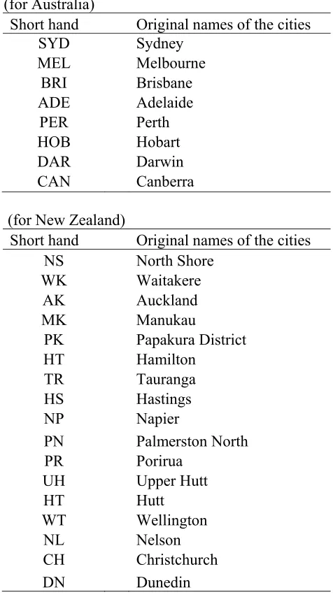
well for New Zealand housing stock, as shown in the Appendix A. The geographic locations of
these cities are presented in Figure 2.
< Figures 2a, 2b about here>
11
The ABS website (http://www.abs.gov.au) provides very detailed explanation on the construction of their house
price data and other data series.
12
9
Since we have access to transaction-level data in New Zealand, extra efforts have been
invested in the construction of the house price series.13 The local house price indices estimated
as such are then deflated by the consumer price index (CPI) to derive the real house price
indices.
We obtain monthly rental data for detached or semi-detached houses from the Tenancy
Services Division of Department of Building and Housing (DBH) in New Zealand. Under the
Residential Tenancies Act, all tenancy bonds must be lodged with the DBH within 23 working
days from the tenancy start. The bonds normally amount to two or three weeks of rents payable
under the new tenancy. The DBH rental data is transaction based and very comprehensive in
terms of recording the market rent settings for all new residential tenancies in New Zealand. We
first calculate the monthly median rent, and then construct rental indices for each local housing
market. The estimated rental indices are then deflated by CPI and should represent the local
market supply and demand factors for housing.
National economic variables such as real GDP, CPI, population, unemployment rate, and net
migration, are available from Statistics New Zealand.14 For the quarterly reported aggregate
data such as real GDP, CPI and unemployment data, we have interpolated them on a monthly
basis. Monthly net migration is calculated on per 1000 people of the existing population.
Monthly interest rate, exchange rate and bank loan data are obtained from the Reserve Bank of
New Zealand. Stock market price movements are obtained from Datastream. We use the
10-year government bond rate to represent the interest rate for housing, simply because of the
long-term nature of owning. For the exchange rate, it is expressed as the New Zealand dollar against
13
For instance, as the repeat sales method is vulnerable to outliers (Meese and Wallace, 1997), we use prior knowledge to eliminate all multiple sales where the second sale price is less than 0.7 or more than 2.5 times the first sale price. Moreover, since the QV data includes building consent information for all the studied cities except Auckland City, we further eliminate the quality changed repeat sales, thus minimizing the constant quality problem faced by the standard repeat sales method. In New Zealand, building consent data is collected for revaluation purposes only where QV is the valuation service provider for the Council. For Auckland City, QV is not the valuation service provider for the council and for that reason there is no building consent data for Auckland City.
14
10
the US dollar. The interest rate, exchange rate, bank loan and stock prices data are then deflated
by CPI to derive their real terms. In the regression, we follow the literature and use log real
exchange rate.15
Finally, we obtain the commodity prices through various sources. As shown in the appendix,
the composition of commodities being exported from Australia and New Zealand are very
different. To facilitate a comparison of results, we use the relative weights of Chen and Rogoff
(2003) for Australia, whose details are reproduced in the Appendix. For New Zealand, we use
the ANZ export commodity price index, which is expressed in US dollars for spot market
non-energy commodity prices. The ANZ index starts in January 1986 and is reported on a monthly
basis thereafter. The index weights are based on the contributions of each commodity to
merchandise exports in New Zealand and adjusted annually. For spot market energy commodity
prices, we obtain them from Datastream. For robustness check, we have also built our own
futures market energy and non-energy commodity prices following Chen and Rogoff (2003).
Futures market commodity prices are obtained from Datastream and Global Financial Database.
Due to the data availability our own futures market non-energy commodity price index starts
from January 1998. All commodity prices are then converted into their real terms by the CPI
adjustment.
4.
Empirical Results
4.1. Testing for unit roots
It is well known that regressions with non-stationary variables can be spurious.16 Therefore,
we first carry out the unit root tests to all economic variables in order to determine their orders
15
The rationale is well known. If we define X to be the real exchange rate of the New Zealand goods against the
US goods, and run two regressions, Y a bX(control)U, and Y a' b'(1/X) ( control)U'.
We will find that in general, b1 / 'b . On the other hand, if we replace Xby lnX , it is easy to show that
'
11
of integration and hence properly de-trend the variables when necessary. Table 1b provides the
full names of the cities and the corresponding short-hand that we are going to use throughout
this paper. Appendix A shows that the 17 cities in our sample represent the majority of both the
population and the number of housing units in New Zealand. It also shows the detailed results
from standard augmented Dickey-Fuller (ADF) test for the time series employed by this study.
It suffices to say that most series are difference-stationary.17 Thus, we will use the
first-differenced version of those series in our regression.
<Table 1b about here>
4.2. Commodity prices and national economic variables
Our first stage regression estimates the relationship between commodity prices and national
variables (properly de-trended when needed). In general, the national economic variables of
Australia are not as persistent as New Zealand. The details are reserved in the appendix and we
only highlight the effect of commodity prices on national economic variables in Table 2.
<Tables 2a, 2b about here>
Table 2a presents the results of Australia and Table 2b presents the counterpart of New
Zealand. To have a compact presentation, we will put “S” (“F”) in the cell if spot (futures)
market commodity price is found to be statistically significant in influencing the corresponding
variable. Thus, it is possible to have both “S” and “F” in the same cell, or have neither of them
as well. We use + or – to denote whether the relationship is positive or negative.18
Several observations are in order. First, there are some degrees of consistency in the case of
Australia, both energy and non-energy commodity prices would have a positive effect on the
16
Among others, see Hamilton (1994) for a detailed analysis.
17
It means that the original series are non-stationary, but become stationary after first-differencing. See the appendix A for more discussion on this.
18
12
GDP growth rate and the real interest rate, and a negative effect on the debt-to-GDP ratio. The
real exchange rate is somehow troublesome. When we use spot market commodity prices, we
find that lag energy commodity price is positively correlated to the real exchange rate change
while current period non-energy commodity price is negatively correlated to the real exchange
rate change. In the robustness section, we will examine alternative specifications and study the
overall effect of commodity prices on the local house prices.
Second, using spot market commodity prices may give different results than using futures
market commodity prices. And commodity prices seem to affect different national economic
variables in different countries. For Australia, spot market commodity prices would affect the
change of unemployment, change of real interest rate, change of real exchange rate and change
of real stock price. However, when futures market commodity prices are used instead, the effect
on the change of unemployment rate and change of real stock price will disappear. Instead,
futures market commodity prices are found to influence real GDP growth rate, change of
debt-to-GDP ratio, and net capital flow-debt-to-GDP ratio, in addition to the effect on change of real
interest rate and change of real exchange rate.
For New Zealand, spot market commodity prices are found to influence real GDP growth
rate, change of unemployment rate and change of real interest rate. When futures market
commodity prices are used instead, then only change of unemployment rate and change of real
exchange rate are affected.
There are many potential reasons for the difference in results. First, futures market
commodity prices are not perfect predictors of the subsequent period spot market counterparts.
In addition, the contents of commodity exports vary across countries. Hence, “energy
commodity price index” in different countries has different statistical properties and may
13
participation in spot versus futures market is different. Limited by space, we reserve the details
in the appendix.
In sum, the results from Tables 2a and 2b have supported our hypothesis that commodity
prices have an effect on national economic variables. We now proceed to the next stage of the
regression, which examines whether commodity prices would impact the regional economic
variables, controlling for the national variables.
4.3. Commodity prices and local economic variables
Our second stage regression estimates the impact of commodity prices on local economic
variables such as the local housing market rent, controlling for the effect of the national
economic variables. To achieve this, we used the “commodity price-filtered” national variable
from the first stage regression in our second stage regression. Again, the details are reserved in
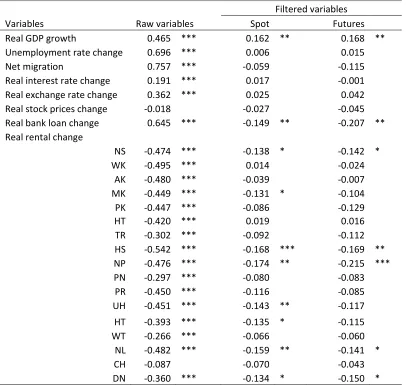
the appendix and we only highlight the impact of commodity prices on local rent in Table 3.
And to facilitate the comparison, our notations in Table 3 are consistent with that in Table 2.
<Tables 3a, 3b about here>
Table 3a presents the results in Australia. It is clear that when spot market commodity prices
are used, none of the city rent series is affected by the commodity prices. When futures market
commodity prices are used instead, the effect on rent in Adelaide, Brisbane, Darwin and Perth
are all in-significant. Decisive results come from Canberra and Sydney, where lagged
non-energy commodity price is found to exert a positive and statistically significant effect on the
rent. While lagged energy commodity prices impact the rent in Hobart negatively, the lagged
non-energy commodity prices impact the rent in Hobart positively. The case of Melbourne is a
bit confusing. While current period non-energy commodity price has a negative effect on the
rent in Melbourne, the lagged non-energy commodity price carries a positive effect. This could
14
and the landlords and renters may not hedge on the same side. Unfortunately, we do not have
access to personal financial portfolio to verify this conjecture and can only leave these for the
future research to pursue.
The case of New Zealand is very clear. For most cities, their rents are affected by neither
spot market nor futures market commodity prices. For the spot market, only the non-energy
commodity price can affect (positively) the rent in North Shore and Manukau. For futures
market, the energy commodity price affects (negatively) the rent in Hamilton and Palmerston
North.
In sum, our second stage regression does not perform as good as the first stage. One
possibility is that there are strong correlations among the rents in different cities and our
formulation does not capture that. In the appendix, however, we show that the rents among
different cities in Australia, as well as among those in New Zealand are not significantly
correlated in general.19 An alternative explanation is that the rental market adjusts slowly and
hence it would react to further past (rather than immediately past) of the aggregate economy.
However, our sample is relatively short and does not allow for including more lags in the
regression with all these filtered variables. It is also possible that the rent is determined by some
other variables such as the bargaining power between the landlords and tenants.20
Unfortunately, among the dataset accessible to us, we do not have the appropriate variable to
capture that.
19 And for those pairwise correlations that are statistically correlated, the numerical values typically do not exceed
0.3, which suggests that the correlations are really not that strong. And since they are not very strongly correlated, even if we replace the filtered macroeconomic variables by some “common factors” or principal components, it may not improve the results significantly.
15
4.4. Commodity prices and local house prices
Our third stage regression attempts to quantify the effect of commodity prices on local
house prices. For the interest of the space, we would first present the results from pooled
regression. And we will then highlight some findings when the city-level house prices are
regressed individually. Tables 4a and 4b present the results when local house prices are pooled
and regressed against commodity prices, the filtered national variable from the first stage
regression, and filtered and pooled local economic variables (rents) from the second stage
regression. Since seasonality is an important feature for the house prices in both countries, we
have added the quarterly seasonal dummies for the regression of Australia and monthly seasonal
dummy variables for the case of New Zealand.
<Tables 4a, 4b about here>
In Table 4a, the dependent variable is the city-level house price in Australia. The first
column presents the results when spot market commodity prices are employed and the second
column presents the results when futures market commodity prices are used instead. The results
in the two columns are consistent with each other. The signs of the coefficients are typically the
same, and even the numerical values are close in many cases. First, it is clear that the lag real
house price change has a positive effect on the current period house price change, which is often
termed as “momentum effect” in the literature. The magnitude is about 0.3 and hence it is not
that large. The signs of the estimated coefficients are mostly expected. Unemployment has a
negative effect on house price because a higher unemployment would mean fewer buyers and
more sellers in the market, which would depress the house price. External debt and net capital
flows have positive effects on the house price as buyers are borrowing from abroad, probably
through financial intermediations and compete for houses, and the house price rises as a result.
16
flow that house-investors would receive and it seems reasonable to expect that the two are
positively correlated. A seasonal dummy is statistically significant as well.
In the appendix, we illustrate that the coefficients for the commodity prices would be the
total effect of the commodity prices on the local house prices, when (filtered) national variables
as well as (filtered) city level rent are used as control. Table 4a suggests that energy commodity
price has no impact on the local house price. On the other hand, non-energy commodity price in
the spot market has a positive effect on house price. In the appendix, we conduct the regression
on each city’s house price on the same set of explanatory variables separately, and find that the
result is mainly driven by three cities: Adelaide, Canberra and Perth. This result may not be
surprising given the economic structure of these cities. For instance, in the state of Western
Australia, where Perth is located, the gross state value added is about 236 billion Australian
dollars in the year 2011-12, where Mining alone contributes 83 billion (Australian Bureau of
Statistics, 2012). It seems reasonable to expect that commodity price fluctuations can have
significant impact on the local house prices.
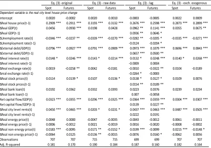
Table 4b shows the results of New Zealand, which are similar. The results of using spot
market and futures market commodity prices are similar qualitatively, and the results are
quantitatively more significant with spot market prices. National variables such as migration,
real interest rate, real exchange rate, real bank loans, as well as local variables such as local
house rents all have statistically significant impacts on local house prices. The effect of
non-energy commodity price on local house price is also positive and statistically significant. In the
appendix, we report the results that each city’s house price is estimated separately. We find that
the non-energy commodity prices are influential to the house prices in four cities, Auckland,
Hamilton, Manukau and Wellington. The appendix also shows that Auckland and Manukau
17
conclude that the commodity price movements are indeed important for house price movement
in New Zealand, at least to a significant part of the population.
Comparing Tables 4a and 4b, we find two obvious differences. First, the sign of previous
house price change is positive in Table 4a, but becomes negative in Table 4b. The results
suggest that house price movements in New Zealand display some kind of mean reversion.
Notice that our estimation results of Australian are based on quarterly data while that of New
Zealand are from monthly data. The variations in the institutional settings (such as the real
estate agency regulations, the bank loan application and approval procedures, etc.), the conduct
of monetary policy (for instance, how strict the central bank follows the “inflation-targeting
policy”) as well as economic structure may also contribute to the difference in estimation
results.
Interestingly, real interest rates are positively correlated to real house price changes both in
Australia and New Zealand. This may be related to the inflation-targeting monetary policy
adopted by the two countries. For instance, let us consider a positive productivity shock. It will
lead to a higher economic growth rate in the short run and possibly a higher inflation rate. In
response to that, the central bank would increase the nominal interest rate aggressively so that
the real interest rate also increases.21 At the same time, a positive productivity shock would also
stimulate the housing demand. Since the housing supply is almost inelastic in the short run, the
house price would also increase. This could lead to a positive correlation between the interest
rate and the house price. However, there may be more than one reason why the real interest rate
and the house price are positively correlated, and we leave this to future research for further
investigation.
21
18
Perhaps more importantly, we find that, once we control for the effect of the
macroeconomic and local economic variables, energy commodity prices are not important in
determining the local house prices, both in Australia and New Zealand. This result holds
whether we use spot market or futures market commodity prices. On the other hand, non-energy
commodity prices have statistically significant and positive effect on the local housing prices.
Again, the result holds whether we use spot market or futures market commodity prices. These
results seem to be intuitive. For Australia, the export of energy commodities used to be less than
20% of total export until recent years. For New Zealand, most exports are non-energy
commodities. Hence, an increase in the non-energy commodity prices would have a similar
effect as a positive productivity shock, which would encourage the local house prices to
increase. It confirms our earlier conjecture that commodity price shock can impact local house
prices as a positive “income shock”, rather than a negative “cost shock” as emphasized by some
previous literatures. Since the energy and non-energy commodity price fluctuations generate
very different results, this paper also confirms the findings of Chen and Rogoff (2003) that it is
important to consider the two commodity prices separately. In particular, our empirical results
seem to suggest that energy commodity prices seem to have a larger effect on the
macroeconomic variables, and yet at the end have an almost neglectable overall effect on the
local house prices, while non-energy commodity prices seem to affect the local house price
directly. Thus, our results seem to justify our conjecture that the local house prices of some of
the cities in Australia and New Zealand are “commodity house prices” as their currencies are
“commodity currencies”.
4.5. Dynamic Analysis
In this section, we would investigate how a change in the commodity prices would affect the
19
However, since commodity prices are exogenous variables in our econometric model, strictly
speaking, we cannot apply the traditional IRA. Nonetheless, the simple structure we adopted
here allows us to study the dynamic effect of (global) commodity price change on the city-level
house prices.22 The following proposition formalizes the idea.
Proposition 1
Based on the regression equation (1), (2) and (3), we can derive the following formula,
(4)
where L is the lag operator, and hence we can describe how an once-and-for-all change in the
commodity prices,
ct P
, would affect the local house prices.
(The proof and the details formulas for the matric polynomials, C Li
, i1, 2,... can all befound in the Appendix ).
Equipped with these formulas, we can analyse how a change in the commodity prices would
affect the local house prices. For instance, to investigate how a change in the energy commodity
price would affect the local house price, we simply set ∆ , where is the
standard deviation of the de-trended energy commodity price . Clearly, this is in parallel
to the traditional IRA, where the innovation term would be taken as a standard deviation of the
shock. Similarly, we obtain the effect of non-energy commodity prices on house price changes
by setting ∆ . As an illustration, we will only present the case of one standard
deviation increase in the spot market commodity prices, and the case for futures market
counterpart can be studied similarly. To make our dynamic response analysis more compatible
with the traditional IRA as well as to facilitate comparison across cities, we “normalize” the
22 A merit of this approach is that since commodity prices are exogenous variables in the system, we may not worry
20
house price changes, which is to divide the estimated house price change by the mean of the
same city house price. We will present the dynamic responses of the city level house prices of
all 8 cities of Australia. For the case of New Zealand, since it is too burdensome to study the
impacts of 17 cities, we will focus the three major cities of New Zealand, Auckland (AK),
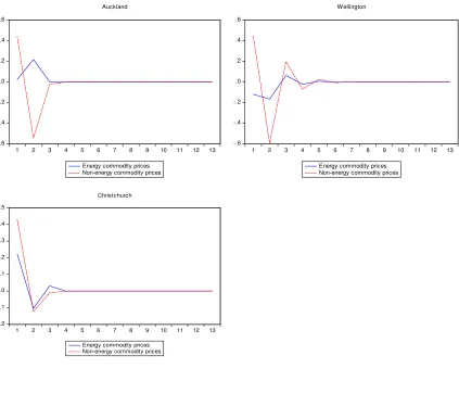
Wellington (WT) and Christchurch (CH).23 The results are presented in Figure 3.
<Figures 3a, 3b about here>
In Figures 3a and 3b, y-axis plots the percentage change of house price, ∆ , / in
Australia and New Zealand respectively, where is simply the time-average of , . The
x-axis is the time periods (months). To facilitate the comparison, we plot the responses of
city-level house prices to change in energy commodity price as well as non-energy commodity price
in one graph. Several observations are immediate from Figure 3a. First, in terms of percentage
change, in most of the Australian cities, the responses to non-energy commodity price are much
bigger than the energy counterpart, consistent with our results in Table 4a. Second, in most of
the Australian cities, an increase in the energy commodity price typically generates a
hump-shape response in house price, i.e. the house price will first increase and then decrease. This is
somehow similar to what the business cycle literature found with “productivity shock”. Perth is
an exception. Its house price will drop first and then bound back. It may be related to the fact
that Perth may be economically and geographically different from other cities.
Notice that the local house prices typically “overshoot” in response to an increase in the
non-energy commodity price, i.e. the initial positive effect on house price generated by the
“shock” will die off over time, even becomes a negative response in house price, and then
23
21
restore to “normal”.24 Such “over-shooting” behaviour is different from that in the exchange
rate market. In the international finance literature, it is well-known that when the nominal prices
are sticky in the short run, the exchange rate may over-shoot, meaning that the short run
adjustment is more than the long run adjustment. Here the key is instead the sluggish housing
supply. Since the supply of housing cannot adjust quickly to a positive commodity price shock
(as an income shock), the local house price increases. Over time, new housing supply arrives at
the market and drives down the house price.25
Figure 3b shows the case of the 3 selected cities in New Zealand. It is clear that they behave
very differently. For instance, an increase in non-energy prices will generate a hump-shape
response in the local house price all three cities, Auckland, Wellington, and Christchurch. On
the other hand, when there is a positive shock in the energy commodity price, the local house
prices of the three cities behave very differently. In Auckland, a momentum of positive
responses will build up and then die off, which is qualitatively like a mirror image of the
response to non-energy commodity price shock. For Wellington, the response to energy
commodity price is qualitatively similar to the response to non-energy commodity price shock,
except that the magnitude will be much smaller. For Christchurch, the house price responses to
both energy and non-energy commodity prices are very similar, both qualitatively and
quantitatively. These differences in house price responses may be due to the differences of the
city economies. Auckland is the largest city of New Zealand and a large share of local economy
is related to commercial activities, including the trading of energy-related commodities.
Wellington is closely linked to government agency and surrounding industrial production. On
the other hand, Christchurch is largely agricultural orientated.
24
We are aware that Hobart is an exception. We lack more detailed city level data to investigate the reason, and can only leave this to future research.
22
In sum, we can conclude that the house price dynamics driven by a change in energy
commodity price can be very different from that generated by the non-energy counterpart,
depending on the local economic structure. And we find that similar patterns emerge from both
Australian and New Zealand cities, which are somehow commodity-export dependent. This
may be worth further attention for theoretical modelling. Obviously, this research benefits a lot
from using 8 Australian and 17 New Zealand cities in the analysis. In other words, our
hierarchical and dis-aggregate approach may help us to uncover the mechanism through which
the global commodity market affecting local house prices.
These observations are clearly at odds with traditional RBC (Real Business Cycles) type
models where there is only one shock which drives the economy. At the same time, they seem
to give support to the approach of DSGE model, which emphasizes the differential responses of
the economy under different shocks.26 In addition, this paper adds weight to the position that we
should analyse the effect of energy-related commodity price shocks separately from the
non-energy-related commodity price shocks.
5.
Robustness checks
5.1 What does “filtering” do to the data?
This section attempts to accomplish a few tasks. First, we will show that our approach of a
3-stage regression is indeed important. As a starting point, we first compare the raw data series
with the “filtered” counterparts. When we “filter” or “remove” the effect of commodity prices
on the national or regional economic variables, do we change the behaviour of those variables
significantly? To put it in another way, if the raw data and the filtered data are very similar, then
whether regressing the raw data or filtered data in the second and third stage would not make
26
23
much difference and hence the 3-stage regression approach proposed here may have limited
value-added. Table 5 shows the correlation between the raw data and the filtered data. Notice
that while we have only one raw data series, our models generated two filtered data series, one
is the residual term when the national economic variables are regressed against spot market
commodity prices, and another is when the national economic variables are regressed against
futures market commodity prices (see Table 2). Therefore we can calculate the correlations
between the raw data and the data series filtered by spot market commodity prices, as well as
that between the raw data and the data series filtered by futures market commodity prices. The
two correlations are reported in two different columns in Table 5.
<Tables 5a, 5b about here>
First, whether we filter the data with spot market data or futures market data does not make
very significant difference for both Australia and New Zealand. Second, it seems that different
national variables show very different results. For instance, in the case of Australia, Table 5a
shows that the correlations between the raw and filtered data of GDP growth rate,
unemployment, and debt-to-GDP ratio are below 0.7, suggesting that they may be exposed more
to changes in the commodity prices. For real interest rate change and real exchange rate change,
the correlations are between 0.7 to 0.8, suggesting that they may be less influenced by the
commodity price movements. For the stock price, bank loans and capital flow-to-GDP ratio, the
correlations are 0.9 or above, suggesting that they are almost immune to the fluctuations of the
commodity prices. The correlations among the raw data and the commodity price-filtered-data
of most regional rental change are between 0.7 to 0.9 (except Sydney), suggesting the
commodity prices on these variables are mild. The difference in these correlations also provide
further hints on the channels through which the commodity prices fluctuations in the
24
A comparison of Tables 5a and 5b might suggest that these channels may be
country-specific. Table 5b shows that the correlations among the raw and filtered data for different
national level variables of New Zealand. It is clear that while the correlations are still below 0.7
for unemployment, the correlations are above 0.8 for GDP growth, which is very different from
the case of Australia. At the same time, the correlations for net migration are below 0.7 and that
for bank loans are around 0.7, suggesting that commodity price fluctuations may affect the local
house price through changing these variables. On the other hand, real interest rate change, real
exchange rate change and real stock price change do not seem to be affected by the filtering of
commodity prices, as the corresponding correlations among the raw and filtered data are close
to or above 0.9. And for most regional rental changes, the correlations among the raw data and
the commodity price-filtered-data are in the range of 0.8 to 0.9. It suggests a minor impact of
the commodity prices to these regional variables.
To shed further light on the exact effects of the filtering procedure on the data series are, we
calculate the serial correlations of all three series: the raw data, the data series filtered by spot
market commodity prices, and the one filtered by futures market commodity prices, and report
the results in Tables 6a and 6b.
Several “stylized facts” are obvious. The raw data are significantly correlated and that
justifies the inclusion of lagged terms in the regressions.27 On the other hand, the filtered data of
Australia are not serially correlated in general, whether the data is filtered by spot commodity
prices or futures commodity prices. For New Zealand, some of the national level data are still
serially correlated after filtering. Yet although the correlations may be statistically significant,
27
25
their numerical values are around 0.2 or less. Thus, the filtering process significantly reduces, or
even removes, the autocorrelation in the national level variables in Australia and New Zealand.
<Tables 6a, 6b about here>
5.2 Raw data versus filtered data
The previous section studies the effect of filtering onto the national and regional economic
variables. It seems natural for this section to re-examine the effect of commodity prices on the
local house prices if the raw data, instead of the filtered version, have been used in the analysis.
Thus, our robustness check continue to use the (city-level) local house prices as dependent
variable and we compare the results of using the raw data, adding the lagged filtered variable in
equation (3) and (later) by treating the exchange rate as an exogenous variable with the 3-stage
regression approach proposed by this paper. To facilitate the comparison, we reproduce the
results in Table 4 as the first two columns of Table 7. In the third and the fourth columns of
Table 7, we use the raw data instead of the filtered ones. The results of Australia are reported in
Table 7a and those of New Zealand in Table 7b. With this side-by-side comparison, several
observations are in order. First, in general, the effects of macroeconomic variables on the local
house prices are similar. Second, the statistical significance of the local house rent is much
weakened (for the case of Australia) or even disappear (for the case of New Zealand) when the
raw data rather than the filtered data is used. Thus, using our 3-stage regression approach does
alter the economic conclusion. Third, the energy commodity prices do not seem to matter for
local house prices, whether in Australia or in New Zealand. Fourth, the effect of non-energy
commodity prices seems to be the same for Australia. For New Zealand, as evident in Table 7b,
the point estimate for the effect of non-energy commodity prices are significantly reduced. For
26
0.0855 (3-stage regression) to 0.0582 (raw data). For the futures market counterpart, the
estimated coefficient drops from 0.0465 (3-stage regression) to 0.0295 (raw data). These
observations again confirm the general finding that it is indeed important to use a multi-step
procedure to estimate the effect of international commodity price on the local house price.
<Table 7a, 7b about here>
The fifth and sixth columns of Table 7 present the results after including the lagged variable
of filtered data in equation (3) (see the columns under Eq. (3) – lag). Again, Table 7a presents
the results for Australia and Table 7b for New Zealand. Interestingly, the city rent becomes
statistically significant again, and most estimated coefficients are similar. Overall, all these
suggest that our filtering procedure is indeed important to uncover the relationship between
commodity prices and city-level local housing prices in New Zealand.
5.3. Exogenous versus endogenous exchange rate
We also modify the original formulation and re-run all the regressions as a robustness
check. Specifically, the modified formulation treats the exchange rate as an exogenous variable
instead of an endogenous variable, which is the case considered earlier. This change in
formulation is motivated by the results in Chen, Rogoff and Rossi (2010) that “commodity
currency exchange rates have surprisingly robust power in predicting global commodity prices,”
yet the “reverse” relationship (commodity prices forecasting exchange rates) is less robust.
Formally, our modified model is written as follows:
= + + + + + (7)
where the change of log real exchange rate, Et , is no longer included in the vector of national
variables Vtn, but instead is included on the right hand side as an exogenous variable.
27
, = + + + + + + , + , , j = 1, 2, … (8)
And then in the third stage, we have
, = , + , + ∑ , + + , + + + ∑ + ,
j = 1, 2, … (9)
Now we have to control for the persistence of house price, , for the filtered national
variables, , for the commodity prices, for the change of the log real exchange rate,
which should cover all different possibilities.
The last two columns of Tables 7a and 7b present the results when the changes of log real
exchange rates are treated as an exogenous variable (see the column under Eq. (3) – exch.
exogenous). Again, except for the point estimate of the effect of non-energy commodity price in
the futures market on the local house price, the results are similar to the original estimation (the
first and second columns). For the case of Australia, the coefficient of the spot market
non-energy commodity price changes from 0.0183 (when exchange rate is treated as an endogenous
variable) to 0.0215 (when the exchange rate is treated as an exogenous variable). For the case of
New Zealand, the change is more significant. The coefficient of the spot market non-energy
commodity price changes from 0.0855 (when exchange rate is treated as an endogenous
variable) to 0.0629 (when the exchange rate is treated as an exogenous variable), while
maintaining 1% significant level.
Putting all these together, we can safely conclude that the influence of the commodity prices
on at least some cities in Australia and New Zealand local house prices are significant and
robust. In addition, our 3-stage estimation procedure contributes in uncovering such a
relationship.
28
Commodity price movements have gained attention in international media such as Wall
Street Journal, Financial Times, Economist magazine, etc. in the rent years. They are often
perceived as problems to be solved. Recent researches such as Chen and Rogoff (2003), Chen,
Rogoff and Rossi (2010), amongst others, take advantage of those movements and use them to
enhance our understanding of the business cycles in some “commodity dependent economies”.
This paper follows this approach and uses the commodity price movements to identify the
mechanism for “external shocks” to affect the local house prices. We develop a simple,
geographically hierarchical empirical model for Australia and New Zealand economies as well
as their cities. We find that an increase in commodity price functions like a positive “income
shock” to these commodity dependent economies which would increase the economic growth
rate and suppress the unemployment rate, rather than a “cost shock” which tends to have the
opposite effect. We also derive analytical results to capture the dynamic responses for
commodity prices to influence the local house prices. We find that commodity prices are
important to local house prices. In particular, energy commodity price shocks tend to affect the
movement of macroeconomic variables, while non-energy commodity price shocks tend to
affect the local house prices more directly. Significant regional heterogeneity is also recognized.
It is also important to separate the price shocks from energy commodities from non-energy
commodities.
As we discussed in the introduction, it is possible that different levels of government impose
policies to “counteract” the effect of commodity price changes. It seems plausible that would be
the case for energy price changes, as it typically triggers inflation and inflating-targeting central
banks would respond. In fact, our hierarchical model can also be interpreted as the reduced form
of a more elaborated model in which economic policy; whether in the form of monetary or
fiscal (both at the national and regional level) would respond to the changes of commodity
29
coefficients may be a combination of the coefficients in the “policy reaction functions” and the
“genuine economic fundamentals”. Thus, future works may further explore how we would
separate the possible (endogenous) policy effect from the pure economic response of the
market.28
Clearly, future research can be extended in other directions as well. First, we can follow
Chen and Rogoff (2012) to cover more countries and examine how commodity prices may
affect the exchange rates in different countries. We also notice that the local house price
responses to commodity price shock seem to depend on the local economic structure. Thus,
future research may investigate a more formal way to categorize and quantify such differences
and may thus build a deeper linkage between real estate researches to regional economic studies.
In addition, our empirical results can be taken as “stylized facts” which would inform
further theoretical modelling, for instance, along the line of open economy DSGE models. The
geographically hierarchical empirical model developed here can be modified for other
“exogenous shocks” and applied to other economies. In fact, our modelling strategy may also
suggest a deeper linkage between house price movements which is traditionally studied in the
field of “urban economics” and international asset pricing, which is traditionally studied in the
field of “international finance”. The globalization may have changed the trade barriers among
countries, as well as the research barriers among fields.
30
References
Aizenman, J. and Y. Jinjarak, 2009. Current account patterns and national real estate markets. Journal of Urban Economics, 66(2), 75-89.
Alexander, C. and M. Barrow, 1994. Seasonality and cointegration of regional house prices in the UK. Urban Studies, 31(10), 1667–1689.
Alquist, R. and L. Kilian, 2010. What do we learn from the price of crude oil futures? Journal of Applied Econometrics, 25(4), 539-573.
Australian Bureau of Statistics, 2012. 2011-12 Australian national accounts—state accounts. Downloaded from www.abs.gov.au
Bardhan, A. D., R. H. Edelstein and C. Leung, 2004. A note on globalization and urban residential rents. Journal of Urban Economics, 56(3), 505-513.
Bardhan, A. D., R. H. Edelstein and T. Tsang, 2008. Global financial integration and real estate security returns. Real Estate Economics, 36(2), 285-311.
Bernanke, B. and A. Blinder, 1992. The Federal Funds rate and the channels of monetary transmission. American Economic Review, 82(4), 901-921.
Bernanke, B. and I. Mihov, 1998. Measuring monetary policy. Quarterly Journal of Economics, 113(3), 869-902.
Bodenstein, M., L. Guerrieri and L. Kilian, 2012. Monetary policy responses to oil price fluctuations. University of Michigan, mimeo.
Bordo, M. D., D. Hargreaves and M. Kida, 2010. Global shocks, economic growth, and financial crises: 120 years of New Zealand experience. NBER Working Paper No. 16027.
Calvo, G. A., 1983. Staggered prices in a utility-maximizing framework. Journal of Monetary Economics, 12(3), 383-398.
Case, K. E. and R. J. Shiller, 1987. Prices of single-family homes since 1970: new indexes for four cities. NBER Working Paper No. 2393.
Catao, L. and R. Chang, 2012. Monetary rules for commodity traders. Rutgers University, mimeo.
Caves, R., J. Frankel and R. Jones, 1999. World trade and payments: an introduction. New York: Addison-Wesley.
Chen, Y. and K. Rogoff, 2003. Commodity currencies. Journal of International Economics, 60(1), 133– 169.
Chen, Y. and K. Rogoff, 2012. Are the commodity currencies an exception to the rule? Global Journal of Economics, 1, 1250004 (28 pages).
Chen, Y., K. Rogoff and B. Rossi, 2010. Can exchange rates forecast commodity prices? Quarterly Journal of Economics, 125(3), 1145–1194.
31
Coleman, A. and J. Landon-Lane, 2007. Housing markets and migration in New Zealand, 1962-2006. Discussion Paper No. DP2007/12. Wellington, New Zealand: Reserve Bank of New Zealand.
Cooley, T. and M. Dwyer, 1998. Business cycle analysis without much theory: a look at structural VARs. Journal of Econometrics, 83(1-2), 57-88.
Davidoff, T., 2006. Labor income, housing prices, and homeownership, Journal of Urban Economics, 59(2), 209-235.
De Gregorio, J., 2012. Commodity prices, monetary policy and inflation. Universidad de Chile, mimeo.
Fernandez-Villaverde, J.; Rubio-Ramirez, J.; Sargent, T.; Watson, M., 2007. A, B, C’s (and D’s) for understanding VARs, American Economic Review, 97, 1021-26.
Franses, P.H., 1990. Testing for seasonal unit roots in monthly data. Rotterdam: Econometric Institute Report No. 9032/A, Erasmus University.
Franses, P. H., 1991. Seasonality, nonstationarity and the forecasting of monthly time series. International Journal of Forecasting, 7, 199–208.
Hamilton, J., 1994. Time series analysis. Princeton: Princeton University Press.
Hamilton, J., 2008. Oil and the macroeconomy, in New Palgrave Dictionary of Economics, 2nd edition, ed., by Durlauf, S., Blume, L., New York: Palgrave McMillan.
Harding, J., S. Rosenthal and C. F. Sirmans, 2003, Estimating bargaining power in the market for existing homes, Review of Economics and Statistics, 85(1), 178-188.
Hanushek, E., S. Rivkin and L. Taylor, 1996. Aggregation and the estimated effects of school resources. Review of Economics and Statistics, 78(4), 611-627.
Jones, R., 1979. International trade: essays in theory. New York: North Holland.
Kan, K., 2002. Residential mobility with job location uncertainty. Journal of Urban Economics, 52(3), 501–523.
Kan, K., 2003. Residential mobility and job changes under uncertainty. Journal of Urban Economics, 54(3), 566–586.
Kapetanios, G., A. Pagan, A. Scott, 2007, Making a match: Combining theory and evidence in policy-oriented macroeconomic modeling, Journal of Econometrics, 136(2), 565-594.
Leung, C. K. Y., 2004. Macroeconomics and housing: a review of the literature. Journal of Housing Economics,13(4), 249-267.
Leung, C. K. Y., 2007. Equilibrium correlations of asset price and return. Journal of Real Estate Finance and Economics,34(2), 233-256.
32
Lubik, T. and W. Teo, 2005. Do world shocks drive domestic business cycles? Some evidence from structural estimation. Economics Working Paper Archive No. 522. Johns Hopkins University, Department of Economics.
Malpezzi, S. and S. Wachter, 2005. The role of speculation in real estate cycles, Journal of Real Estate Literature, 13, 143-164.
Marion, N., 1984. Nontraded goods, oil price increases and the current account. Journal of International Economics, 16(1-2), 29–44.
Meese, R. and N. Wallace, 1997. The construction of residential housing price indices: a comparison of repeated sales, hedonic regression, and hybrid approaches. Journal of Real Estate Finance and Economics, 14(1-2), 51–74.
Otto, G., 2007. The growth of house prices in Australian capital cities: what do economic fundamentals explain? Australian Economic Review, 40(3), 225-238.
Pindyck, R., 2001, The dynamics of commodity spot and futures markets: a primer. Energy Journal, 22(3), 1-29.
Reichsfeld, D. and S. Roache, 2011. Do commodity futures help forecast spot prices? IMF working paper.
Rogoff, K., 2001. Dornbusch’s overshooting model after 25 years. Mundell-Fleming Lecture, IMF.
Sargent, T., 1979. Macroeconomic theory. New York: Academic Press.
Shi, S., M. Young and B. Hargreaves, 2009. The Ripple effect of local house price movements in New Zealand. Journal of Property Research, 26(1), 1–24.
Sockin, M. and W. Xiong, 2013. Feedback effects of commodity futures prices. Princeton University, mimeo.
Walsh, C., 2010. Monetary Theory and Policy, 3rd. ed., Cambridge: MIT Press.
33
34
Figure 2a: Geographic locations of 8 selected cities of Australia
[image:36.612.97.357.348.689.2]35
Figure 3a: Dynamic Response analysis for one standard deviation of spot market commodity prices on city level housing prices – Australia
-1 0 1 2 3 4 5 6
1 2 3 4 5 6 7 8 9 10 11 12 13
Energy commodity prices Non-energy commodity prices
Adelaide -1.2 -0.8 -0.4 0.0 0.4 0.8
1 2 3 4 5 6 7 8 9 10 11 12 13
Energy commodity prices Non-energy commodity prices
Brisbane -1.2 -0.8 -0.4 0.0 0.4 0.8 1.2
1 2 3 4 5 6 7 8 9 10 11 12 13
Energy commodity prices Non-energy commodity prices
Canberra -.10 -.05 .00 .05 .10 .15 .20 .25
1 2 3 4 5 6 7 8 9 10 11 12 13
Energy commodity prices Non-energy commodity prices
Darwin -.3 -.2 -.1 .0 .1 .2 .3 .4
1 2 3 4 5 6 7 8 9 10 11 12 13
Energy commodity prices Non-energy commodity prices
Hobart -2.5 -2.0 -1.5 -1.0 -0.5 0.0 0.5 1.0
1 2 3 4 5 6 7 8 9 10 11 12 13
Energy commodity prices Non-energy commodity prices