Thermo mechanical fatigue testing and simulation using a viscoplasticity model for a P91 steel

(1)

Thermo-mechanical fatigue testing and simulation using a viscoplasticity model

for a P91 steel

C.J. Hyde

a,⇑

_{, W. Sun}

a

_{, T.H. Hyde}

a

_{, A.A. Saad}

b a

Department of Mechanical, Materials and Manufacturing Engineering, University of Nottingham, Nottingham NG7 2RD, UK

b

School of Mechanical Engineering, Universiti Sains Malaysia, 14300 Nibong Tebal, Penang, Malaysia

a r t i c l e

i n f o

Article history:

Received 1 November 2011

Received in revised form 5 January 2012 Accepted 8 January 2012

Available online 1 February 2012

Keywords:

Thermo-mechanical fatigue Viscoplasticity model Material constant optimisation Cyclic softening

a b s t r a c t

An experimental programme of cyclic thermo-mechanical testing for a P91 power plant steel, under isothermal, and in-phase and out-of-phase thermo-mechanical, temperature-strain cycle conditions, has been implemented. Using the experimental data, an optimisation procedure has been developed for the accurate determination of the material constants under isothermal conditions, in which the Chab-oche model is employed to describe material responses. The material was found to exhibit cyclic soften-ing throughout the full life cycles, which is believed to be related to the evolution of microstructure and the propagation of micro-cracks. The model developed shows good predictive capability of cyclic stress– strain behaviour and cyclic softening.

Ó2012 Elsevier B.V.

1. Introduction

Increasing temperatures and pressures for increased efﬁciency and reduced CO2 emissions has become an ongoing trend for

power generation plants. New advanced materials that allow for signiﬁcant increases in operating temperature are essential for this need. Due to the intermittent nature of renewable energy genera-tion, conventional power generation plants are now subjected to a higher frequency of thermo-mechanical cycling, demanded by ﬂex-ible operation. This indicates that more attentions need to be given to the problem of thermo-mechanical fatigue in component life assessment and in the design of new plants.

The need for power generation industry to improve the thermal efﬁciency of power plant has led to the development of 9–12% Cr martensitic steels. The development of and research on P91 steels started since late 1970s and early 1990s, respectively[1]. The work has focussed on their creep strengths due to its intended applica-tion at high temperature. Recently, the introducapplica-tion of more cyclic operation of power plant has introduced the possibility of fatigue problems. Bore cracking due to the effects of varying steam warm-ing has been reported[2]. The temperature cycling causes thermal gradients between the inside and outside of components and this can cause cyclic stress levels to be of concerns. Recently, research on thermal–mechanical analysis of P91 has been carried out

including the characterisation of the cyclic behaviour of the mate-rial using the two-layer and uniﬁed visco-plasticity models[3,4].

The present paper is concerned with the application of the Chaboche uniﬁed viscoplasticity model to characterising the iso-thermal and iso-thermal–mechanical fatigue responses, and the preli-minary study on the cyclic failure mechanisms of a P91 steel under such conditions.

2. Experimental testing

2.1. Equipment and experimental procedure

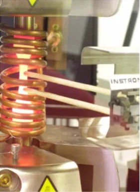
Fig. 1the test set-up used for the isothermal and an-isothermal

cyclic testing performed on the P91 steel. It can be seen that the heating method used is an RF induction coil and that the test strain is measured using a ceramic rod extensometer (all testing is strain controlled, whereRe=1, and the stress response measured).

Fig. 2 shows the specimen geometry used for this testing. It

should be noted that for some testing, central (cooling) holes were not present within the specimens. Strain controlled saw-tooth type waveforms were used for all testing presented in the present work. For all test results shown within the present paper, the strain rates are 0.1%/s for isothermal testing and 0.0333%/s for anisothermal testing. For the anisothermal testing the temperature rates are 6.67°C/s.

All testing performed under an-isothermal conditions was per-formed under either in-phase (IP) or out-of-phase (OP) conditions, shown by parts (a) and (b) ofFig. 3respectively.

0927-0256 Ó2012 Elsevier B.V. doi:10.1016/j.commatsci.2012.01.006

⇑ Corresponding author. Tel.: +44 (0)115 9513735.

E-mail address:[email protected](C.J. Hyde).

Contents lists available atSciVerse ScienceDirect

Computational Materials Science

j o u r n a l h o m e p a g e : w w w . e l s e v i e r . c o m / l o c a t e / c o m m a t s c i

Open access under CC BY license.

(2)

2.2. Test materials

All testing presented within the present work has been per-formed on a P91 steel for which the chemical composition is shown inTable 1.

3. The Viscoplasticity (Chaboche) model

The Chaboche uniﬁed viscoplasticity model[5]has been chosen to represent the uniaxial cyclic material behaviour of the P91 steel. The uniaxial form of the model is as follows:

_

e

p¼

f Z

n

sgnð

r

v

Þ ð1Þ

whereZandnare material constants,

e

pis the plastic strain,f

rep-resents the model yield criterion, described by Eq.(2)in the text that follows,

r

is the stress within the material, as described by Eq.(2)in the text that follows and

v

is the kinematic hardening parameter, described by Eqs.4 and 5. Also:

sgnðxÞ ¼

1 x>0 0 x¼0

1 x<0

andhxi ¼ x x>0

0 6₀

The yield criterion and the total stresses are given by:

f¼ j

r

v

j Rk ð2Þ

r

¼

v

þ ðRþkþ

r

_vÞsgnð

r

v

Þ ¼Eð

e

pÞ ð3Þ

where the elastic domain is deﬁned byf6_{0 and the inelastic} do-main byf> 0, R is the isotropic hardening parameter as described by Eq.(6),kis the initial yield stress,

r

_vis the viscous stress as de-scribed by Eq.(8),Eis Young’s modulus and

e

represents the total strain. The model takes into account both kinematic hardening and isotropic hardening as follows:

_

v

i¼Ciðai

e

_p

v

ip_Þ ð4Þ

v

¼

v

1þ

v

2 ð5Þ

_

R¼bðQRÞp_ ð6Þ

wherei= 1, 2 andb,Q,Ciandaiare material constants.pis the

accu-mulative plastic strain, given by:

_

[image:2.595.88.229.68.261.2]

p¼ j

e

_pj ð7Þ

[image:2.595.136.459.437.574.2]

Fig. 1.TMF machine grips, RF induction coil, test sample and extensometry set-up.

Fig. 2.Specimen geometry (dimensions in mm).

Time (s)

Temperature,

Mechanical strain

Temperature,

Mechanical strain

Time (s)

(a)

(b)

[image:2.595.111.476.612.737.2]

(3)

Fig. 4illustrates the physical meaning of the two types of hard-ening and the effect they have on the yield surface; both types of hardening are shown in three-dimensional (principle) stress space. When the stress state within the material causes the yield surface to be reached, kinematic hardening, implemented by Eqs.4 and 5), is represented as themovementof the yield surface, as illustrated in part (a) ofFig. 4. Isotropic hardening, implemented by Eq.(6)), rep-resents thegrowthof the yield surface, as shown in part (b) of

Fig. 4.

Creep is also accounted for within the model, in the form of the Norton (1929) creep law, as follows:

r

v¼Zp_1=n ð8Þ

Eq.(4), the viscoplastic ﬂow rule, is the basic equation within the model. As can be seen from Eqs.(2)–(8), all of the other model variables, such as those used for calculating both types of harden-ing (isotropic, R, and kinematic,

v

) and viscous stress,

r

v, are

dependent on the value of accumulated plastic strain,p, calculated in turn, as shown by Eq.(7)), from the plastic strain,

e

p, values

ob-tained from this viscoplastic flow rule. Eq.(8)defines the viscous stress and therefore the creep effect within the model. The above model has been implemented, in uniaxial form, within Matlab, a high level programming language. The identification of the final values for material constants requires a step by step procedure. Firstly, the initial values of the parameters are estimated using the experimental results. These initial values are then used to ob-tain an optimised set of material constants in a simultaneous parameter optimisation routine based on two objective functions

(stress–strain loops and the hardening/softening curve). In total, the material model requires the identiﬁcation of 10 material con-stants. The procedure for the determination of the initial material constants from experimental data as well as the subsequent opti-misation procedure for the determination of the ﬁnal material con-stants have been described by[6–8].

4. Characterisation of isothermal and thermo-mechanical behaviour

4.1. Isothermal cyclic and softening behaviour

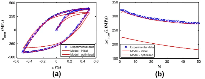
Fig. 5shows examples of comparisons of model predictions to

experimental data at 500°C. Also shown is the improvement in the model prediction due to the optimisation of the material con-stants. It can be seen that the model using the optimised material constants gives extremely accurate prediction of material behav-iour both in terms of the stress–strain loops and the hardening/ softening curves.

4.2. An-isothermal cyclic behaviour

In order to produce an-isothermal behaviour predictions, inter-polation of the material constants with respect to temperature is used.Fig. 6shows example of comparisons of model predictions to experimental data under OP conditions in the temperature range of 400°C to 500°C. As for isothermal conditions, the aniso-thermal model predictions correspond very closely to experimen-tal data.

5. Material degradation under cyclic loading

Microstructural investigations have been performed on the P91 test pieces from the isothermal testing at 600°C. These investiga-tions were performed at various life fracinvestiga-tions in order to observe the evolution of the P91 microstructure throughout the life cycles. Transmission electron microscopy (TEM) and scanning electron microscopy (SEM) were used for the investigations.

Microstructural evolution of the P91 steel under cyclic loading occurs at the sub-grain scale[9].Fig. 7shows the investigation re-sults for the ‘as-received’ material as well as for the tested test Table 1

Chemical composition (wt.%) of P91 steel.

Cr Mo Mn Si Ni V C Cu Nb Co P W S Ti Al Fe

8.49 0.978 0.43 0.37 0.32 0.2 0.11 0.07 0.06 0.02 0.014 <0.02 0.008 <0.002 <0.001 Balance

(a)

(b)

Fig. 4.Schematic representations of hardening behaviour (a) Kinematic, and (b)

Isotropic.

0 10 20 30 40 50

150 200 250 300 350

Experimental data Model - initial Model - optimised

-0.6 -0.4 -0.2 0 0.2 0.4 0.6

-500 -250 0 250 500

Experimental data Model - initial Model - optimised

Δσ

ε

σ

[image:3.595.132.476.597.730.2]

(a)

(b)

Fig. 5.Comparison of isothermal model predictions to experimental data for P91 steel, strain rate = 0.1%/s, (a) Initial tensile curve and ﬁrst loop at 500°C (b) Softening

(4)

pieces at cycle numbers 200, 400 and 656 (parts (a–d) respec-tively). Based on the bright ﬁeld TEM images, the sub-grain sizes at these various stages are 0.383, 0.507, 0.551 and 0.604

l

m, respectively. It can be seen that the sub-grains are coarsened with cycle number, particularly within the initial 200 cycles (also, the stress amplitude decreases non-linearly before achieving a stabili-sation stage at around the 200th cycle). It is difficult to clearly identify the sub-grain evolution, at different life fractions, using SEM. However, the SEM images show that a small number of cracks start to develop as the softening curve begins to accelerate as the test piece begins to fail (shown inFig. 7e). Up to this point, it has been found that the value of the cyclic Young’s modulus in each cy-cle is similar to the initial Young’s modulus. If the modulus value is considered to be an indirect measurement of damage[10], it can be regarded that within this cycle range (i.e. up to the number of cy-cles accumulated up to this point), no significant damage was found. Transgranular cracks were observed at many locations on the test piece which ran to failure (at 656 cycles) and one of these major cracks is shown inFig. 7f. Between the 400th and the 656th cycle, the Young’s modulus values and the stress amplitudes are seen to have decreased. The accelerated cyclic softening behaviour in the final stage of cyclic loading can be associated with the prop-agation of cracks within the material.

6. Discussion and future work

A material constitutive model for a P91 power plant steel under cyclic loading and high temperature conditions has been devel-oped based on the experimental results. The material constants were determined by using an optimisation procedure. The material was found to exhibit cyclic softening throughout the vast majority of the life cycles (occasionally initial hardening was present for a small number of cycles). The constants derived give very good pre-dictions of the stress–strain behaviour in cyclic stress–strain con-ditions up to the end of the stabilized softening stage. Some grain coarsening effects and crack growth identiﬁcation have also

been carried out at various stages during isothermal testing yield-ing results which systematically relate to the test conditions under which they were obtained.

Further work will be carried out to more accurately predict the stress relaxation behaviour and to predict the full stages of the cyc-lic softening behaviour, though a more detailed understanding of cyclic softening mechanisms related to micro-crack/damage for-mation and growth.

Acknowledgements

The authors would like to acknowledge the support of The Energy Programme, which is a Research Councils UK cross council initiative led by EPSRC and contributed to by ESRC, NERC, BBSRC and STFC, and speciﬁcally the Supergen initiative (Grants GR/ S86334/01 and EP/F029748) and the following companies; Alstom Power Ltd., Doosan Babcock, E.ON, National Physical Laboratory, Praxair Surface Technologies Ltd, QinetiQ, Rolls-Royce plc, RWE npower, Siemens Industrial Turbomachinery Ltd. and Tata Steel, for their valuable contributions to the project.

References

[1] P.J. Ennis, A. Czyrska-Filemonowicz, Recent advances in creep-resistant steels for power plant applications, Sadhana – Academy Proceedings in Engineering Sciences, vol. 28, no. 3–4, 2003, pp. 709–730.

[2] S.J. Brett, Service experience of weld cracking in CrMoV steam pipework systems, in: Second International Conference on Integrity of High Temperature Welds, London, 2003, pp. 3–17.

[3] T.P. Farragher, N.P. O’Dowd, S. Scully, S.B. Leen, Thermo-mechanical characterization of P91 power plant componrents, in: Twenty First International Workshop on Computational Mechanics of Materials, 22–24 August, Limerick, Ireland, 2011.

[4] Yunpeng Gong, C.J. Hyde, W. Sun, T.H. Hyde, The Journal of Materials: Design and Applications 224 (1) (2010) 19–29.

[5] J.L. Chaboche, G. Rousselier, Journal of Pressure Vessel Technology-Transactions of the ASME 105 (2) (1983) 153–159.

[6] C.J. Hyde, W. Sun, S.B. Leen, Cyclic Thermo-Mechanical Material Modelling and Testing of 316 Stainless Steel, European Creep Collaborative Committee, Zurich, Switzerland, 2009. pp. 55–69.

-0.6 -0.4 -0.2 0 0.2 0.4 0.6

-400 -200 0 200 400

ε

σ

Experimental data Model - optimised

0 10 20 30 40 50

380 390 400 410 420 430

Δ

σ

Experimental data Model - optimised

[image:4.595.123.462.69.199.2]

(a)

(b)

Fig. 6.Comparison of anisothermal model predictions to experimental data for P91 steel, strain rate = 0.0333%/s, temperature rate = 6.67°C/s, (a) 50th loop under OP

conditions forT= 400–500°C (b) Softening behaviour under OP conditions forT= 400–500°C.

Fig. 7.Bright ﬁeld TEM images for (a) the as-received material, and the subgrain evolution which occurs in ±0.5% strain-controlled test at 600°C for cycle (b) 200th, (c) 400th

[image:4.595.42.546.245.341.2]

(5)

[7] A.A. Saad, C.J. Hyde, W. Sun, T.H. Hyde, Materials at High Temperature 28 (3) (2011) 212–218.

[8] A.A. Saad, W. Sun, T.H. Hyde, D.W.J. Tanner, Procedia Engineering 10 (2011) 1103–1108 (Elsevier).

[9] B. Fournier, M. Sauzay, F. Barcelo, E. Rauch, A. Renault, T. Cozzika, L. Dupuy, A. Pineau, Metallurgical and Materials Transactions A 40 (2009) 330–341. [10] J. Lemaitre, J.L. Chaboche, Mechanics of Solid Materials, Cambridge University