Robust learning from normals for 3D face recognition

Ioannis Marras1, Stefanos Zafeiriou1?, and Georgios Tzimiropoulos1,2 1

Department of Computing, Imperial College London, 180 Queens Gate. London SW7 2AZ, U.K. 2

School of Computer Science, University of Lincoln, Lincoln LN6 7TS, U.K.

{i.marras,s.zafeiriou,gt204}@imperial.ac.uk http://ibug.doc.ic.ac.uk

Abstract. We introduce novel subspace-based methods for learning from the az-imuth angle of surface normals for 3D face recognition. We show that the nor-mal azimuth angles combined with Principal Component Analysis (PCA) using a cosine-based distance measure can be used for robust face recognition from facial surfaces. The proposed algorithms are well-suited for all types of 3D facial data including data produced by range cameras (depth images), photometric stereo (PS) and shade-from-X (SfX) algorithms. We demonstrate the robustness of the proposed algorithms both in 3D face reconstruction from synthetically occluded samples, as well as, in face recognition using the FRGC v2 3D face database and the recently collected Photoface database where the proposed method achieves state-of-the-art results. An important aspect of our method is that it can achieve good face recognition/verification performance by using raw 3D scans without any heavy preprocessing (i.e., model fitting, surface smoothing etc.).

1

Introduction

3D face recognition from 3D surface information has witnessed very rapid develop-ment over the past decade due to the low cost of 3D digital acquisition devices and the need of secure biometrics. Facial surface information has the obvious advantage that it is an intrinsic property of the face and hence more robust to illumination changes than appearance information. On the other hand, 3D face recognition algorithms must be able to handle many challenges such as inaccurate face alignment, pose variations, measurement noise, missing data, facial expressions and partial occlusion.

Many different approaches were proposed for dealing with the aforementioned prob-lems [4, 2, 6, 7, 5, 12]. Early approaches, such as [6], use specific face regions that are not affected by the presence of facial deformations caused by facial expressions, such as the nose and the area around it. An investigation on which face regions should be used for robust 3D face recognition was conducted in [7].

Many methods assume that facial expressions can be modeled, up to a certain ex-tend, as isometries of the facial surfaces [2, 16, 5]. That is, geodesics of the facial surface

?_{The work of Stefanos Zafeiriou has been partially funded by the Junior Research Fellowship}

are approximately preserved in expressive faces. Following this line of research, the al-gorithms [2, 16] compare 3D facial surfaces by computing of iso-geodesic stripes or geodesic lengths between closed curves on the facial surface. Under the same assump-tion, 3D face recognition methods that embed the facial surface into a Euclidean space and replace the geodesic distances by Euclidean ones were proposed in [5]. Using such an embedding, facial surfaces can be matched using conventional methods. The major drawback of these methods is the high computational complexity related to the com-putation of geodesics. Another solution is to an annotated morphable model [12, 14, 3]. One of the drawbacks of these methods is that performance depends on the success of the fitting algorithm which often fails in cases of large expressions or occlusions.

Subspace learning algorithms for normals, such as Principal Component Analysis (PCA), employ low-dimensional representation of surfaces [9, 11, 17, 18]. In its sim-plest form, PCA on surface normals has been applied on the concatenation of normal coordinates [11]. One attempt to exploit the special structure of normals (i.e., that lie on a sphere) was conducted in [17]. In this paper the Azimuthal Equidistance Projection (AEP) was proposed and applied to surface normals prior to the application of PCA. Furthermore, in order to take into consideration the non-Euclidean actual manifold of objects’ surfaces, Principal Geodesic Analysis (PGA) has been proposed [9] for non-linear statistical analysis.

In this paper, motivated by the recent developments in robust 2D subspace learning from image gradient orientations [19], we propose a simple, efficient and robust sub-space learning based on the azimuth angle of face surface normals. We develop a PCA in a space where the normal azimuth angles are mapped by a complex transform into a high-dimensional unit sphere and we demonstrate its robust properties.

The major advantages of the proposed methodology are:

– low-computational complexity. Our algorithms require the eigen-decomposition of Hermitian matrices for training and use simple projections for testing;

– good recognition rates without heavy preprocessing of the 3D meshes (without fit-ting a model). Comparable performance to state-of-the-art was also achieved when combined with this kind of preprocessing;

– state-of-the-art recognition rates in surfaces produced by Shape-from-X and Pho-tometric Stereo algorithms;

– state-of-the-art recognition rates for cases when standard approaches, such as model fitting, may fail (i.e., presence of occlusions).

2

PCA of Needle Maps

Let us define a real surfacef(x)on a lattice or a real spacex= (x, y). The normal field (or needle map) is defined as a set of local surface normalsn(x) = (nx(x), ny(x), nz(x)) that lie on the unit sphere (i.e., ||n(x)|| = 1, where ||.|| is the `2 norm). Mathe-matically, given a continuous surfacef(x), normalsn(x)can be defined asn(x) =

1 q

1+∂f_∂x2+∂f_∂y2

−∂f_∂x,−∂f_∂y,1 T

.

whereΦ : S2 _{7→ <}3_{. On the unit sphere, the surface normaln(x)atxhas elevation} anglesθ(x) =π

2−arcsin(nz(x))and azimuth angle defined asφ(x) = arctan ny(x)

nx(x)=

arctan

∂f ∂y ∂f ∂x

.

Methods for computing the normals of surfaces can be found in [10]. In many cases, surface reconstruction methods do not recover the actual surface but the needle map. Such methods include SfX and PS algorithms [1].

Prior to describing our algorithm, we will briefly outline two popular PCA method-ologies on surface normals that take into account the special structure of surface normals (i.e., that lie in a unit sphere). The first one is based on Azimuthal Equidistant Projection (AEP) [17] and the second one on Principal Geodesic Analysis (PGA) [9, 18].

For simplicity, hereinafter, we assume that we have a setJ = {J1, . . . ,JN}of 3D (or 2.5D) of facial surfaces from a range camera sampled over a grid of resolution

M1×M2. For thei-th facial surface, at each point of the gridx, we compute the normal vectorGi= [ni(x)]∈ PM1×M2wherePis the pure subset of<3of the vector that lies on the unit sphere. In PS and SfX algorithms the setG={G1, . . . ,GN}is computed directly.

2.1 PCA using AEP

In order to formulate AEP we first need to define the mean elevation and azimuthal angle ofGat each spatial locationx. In [17], the mean elevation and azimuthal angles at

xwere defined asθ˜(x) =π₂−arcsin(˜nz(x))andφ˜(x) = arctan_n˜n_˜y(x)

x(x), where˜n(x) =

(˜nx(x),n˜y(x),n˜z(x))is the mean representation of the normal atx. For spherical data, such as surface normals, the intrinsic mean is in many cases represented by the spherical median [8]. For computation ease, in [17], instead of the spherical median, the average surface normal atx ´n(x) =_K1 PK

i=1ni(x), ˜n=

´ n(x)

||´n(x)||was used.

In order to build the AEP, the tangent plane to the unit-sphere at the location cor-responding to the mean-surface normal is computed. A local coordinate system is then established on this tangent plane. The origin is the point of contact between the tan-gent plane and the unit sphere. The x-axis is aligned parallel to the local circle of latitude on the unit-sphere. The AEP maps the normalni(x)atxto the new vector

vi(x) = (vix(x), viy(x))(for more details on how to compute the AEP the interested reader may refer to [17]).

After applying the AEP transform to all the samples ofG, the matrixU= [u1. . .uN] whereui = [vix([1,1]). . . vix([M1, M2])vyi([1,1]). . . viy([M1, M2])]T ∈ <M1M2 is formed. Finally, the method [17] proceeds by computing the eigenvectors of the covari-ance matrix ΣAOP = _N1UUT. These eigenvectors Pare used in order to represent facial shape and used as a prior for SfX algorithms. In order to project a novel sample to the subspace ofP, we first transform the test normal fieldGand˜n(x)intouand then project usingb=PTu.

2.2 Principal Geodesic Analysis

sub-space in which the data lies. In PGA, this notion is replaced by a geodesic submanifold. In other words, while each principal axis in PCA is a straight line, in PGA each prin-cipal axis is a geodesic curve. In the spherical case this corresponds to a circle. PGA utilizes the so-called log and exponential transforms in order to map the normals, that originally lie in a unit sphere, to a space where computing linear variations from the eigenanalysis of a covariance matrix could be meaningful.

In order to formulate PGA first we need to define the exponential and log maps on the sphere and a mean representation of the normals at x. Let ν ∈ TnS2 be a vector on the tangent plane toS2_{atη ∈ S}2 _{andν 6= 0. The exponential map of ν,} denoted by Exp_η(ν), is the point on S2 _{along the geodesic in the direction ofν at} distance||ν|| fromη. The log map is the inverse transform of the exponential map, that is Log_η(Exp_η(ν)) =ν. The geodesic distance between two pointsη1∈ S2and

η₂∈ S2_{can be expressed in terms of the log map, i.e.d(η}

1,η2) =||Logη₁(η2)||. Instead of computing the mean of spherical directional data in [9, 18], PGA finds the intrinsic mean, or the so-called spherical medianµ= [µ(x)]using the Exp and Log mappings. The pointµcannot be found analytically and a gradient descent procedure was used. For details on the computation of the intrinsic mean and the spherical median, the interested reader may refer to [9].

Having computed the spherical medianµit was shown that principal geodesics can be approximated by applying linear PCA on the vectorsuµ= [_νµ(1,1)T. . .

νµ(M1, M2)T]T ∈ <2M1M2whereνµ(x) =Log_µ(x)(ni(x))∈ <2. After the trans-formation of the training setGinto the matrixU= [u1_µ. . .uN_µ]and then we compute the principal components ofΣP GA= _N1UUT. A normal field of a novel sampleGis transformed using Log_µintouµand then projected into the subspaceb=PT_u

µ.

2.3 AAPCA: PCA of Azimuth Angles of Normals

The proposed PCA of azimuth angles of normals, which we call Azimuth Angle Prin-cipal Component Analysis (AAPCA) has been inspired by the use of a complex PCA of image gradient orientations for performing 2D face recognition robust to occlusions and illuminations [19]. In [19] the distribution of differences of gradient orientations between dissimilar images has been studied and it was shown, with extensive exper-iments, that this distribution approximately matches a uniform distribution in[0,2π). It was empirically shown that local orientation mismatches caused by outliers can be also well-described by a uniform distribution which, under some mild assumptions, is canceled out by applying the the cosine kernel. The use of cosine kernel then inspired a complex circular PCA. In the following, we show how this concept can be applied for the case of the azimuth angles of normals. To our knowledge, this is the first time that these concepts are introduced for 3D face recognition.

Let us first define the cosine-based dissimilarity measure between two vectors of az-imuth anglesφi = [φi(1,1). . . φi(M1, M2)]T andφj = [φj(1,1). . . φj(M1, M2)]T as:

d2_(φ

i,φj),

P

x{1−cos[φi(x)−φj(x)]}= 1₂

e

jφ_i−ejφ_j

whereejφi = [ejφi(1), . . . , ejφi(p)]T whereeja = cosa+

√

−1 sina. We define the mapping from[0,2π)M1M2 _{to a subset of complex sphere with radius}√_M

1M2

zi(φi) =e

jφ_{i. (2)}

After transforming the data we apply PCA onzi [19], which we call it Azimuth Angle Principal Component Analysis (AAPCA).

3

Demonstrating the Robust Properties of AAPCA

In order to demonstrate the robustness of the proposed AAPCA we have conducted a series of experiments using artificially generated data. More specifically, we used 21 images of one of the subjects of the FRGC v2 database. Along with this set of images, we created a second one containing artificially occluded images. In particular, 20% of the images ware artificially occluded by a 3D cloth patch placed at random spatial locations (the cloth patch has been taken from one of the images of the FRGC v2 database).

We also evaluated the robust performance of AAPCA quantitatively and compared it with that of PCA on depth values, AEP, and PGA. Because these methods operate on different domains, we used a performance measure which does not depend on the specific domain. More specifically, for each of these methods, we computed a measure of total similarity between the principal subspace for the noise-free caseUnoise-freeand the principal subspace for the noisy caseUnoisyas follows:

Q= k

X

i=1 k

X

j=1

cosαij, (3)

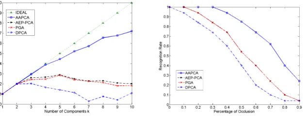
whereαijis the angle between each of thekeigenvectors defining the principal compo-nents ofUnoise-freeand each one ofUnoisy[13]. The valueQlies betweenk(coincident spaces) and 0 (orthogonal spaces) [13]. The meanQvalues over 20 repetitions of the experiment (random placement of the occlusion) and for all tested methods are depicted in Fig. 3(a). The mean values ofQshows that the proposed AAPCA is far more robust that all the other tested methods.

Finally, we evaluated the recognition performance of our algorithm for the case of increasing synthetic occlusions. We used a set of 100 images of 50 persons from the FRGC v2 database and separated it into two sets. Each set contains one image from all 50 persons. All images of the second set (considered as the test set) were artificially occluded by a cloth patch of increasing size. Fig. 3(b) shows the best recognition rate achieved by all tested methods as a function of the percentage of occlusion. As we may observe, our method features by far the most robust performance with a recognition rate over80%even when the percentage of occlusion is about50%.

4

Experimental Results

4.1 FRGC v2

We used the FRGC v2 3D face database [15] for 3D face recognition experiments. The database contains 3D face scans acquired using a Minolta 910 laser scanner that pro-duces range images with a resolution of640×480in pixels. Results on the database are often summarized by the verification rate (VR) at the point of receiver operating charac-teristic (ROC) curve where false accept rate (FAR) is equal to 0.1%. We conducted two experiments. In the first one, we fitted an annotated pre-segmented model in the data [3]. In the second one, we simply aligned the data using the eye coordinates provided by the meta-data of FRGC. The only preprocessing applied was a simple median filter on the depth data. In both types we report the VR at FAR=0.1%for the ROC III (the interested reader for more details on the ROC III may refer in [12, 20]).

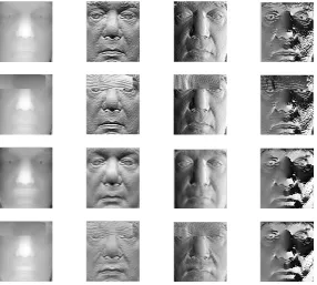
Fig. 1.Quality of reconstruction for`2PCA, PGA, and AAPCA.First row:the original images of (from left to right) depth, the first two components of the normals and the azimuth angle.

Second row:(from left to right) the corresponding occluded images (by the piece of cloth).

Third row:the reconstruction of the images in the first row using the 4 principal components of the non-corrupted subspaces. The first image in the third row shows the reconstruction of the non-occluded depth image (the first image in the first row) using the 4 principal components of`2 PCA. Similarly, the second and third images of the third row show the reconstruction of the first two components of the normals (the second and third images in the first row) using PGA . Finally, the fourth image of the third row shows the reconstruction of azimuth angle using AAPCA.Fourth row:the reconstruction of the occluded set (second row) from the subspaces learned from the corrupted set. For this case, as we may see the reconstruction results,except for the case of the proposed AAPCA, suffer from artifacts.

In the second experiment, where little preprocessing was applied, the proposed method achieved about85%VR at0.1%FAR. This VR is quite good if consider that this result can be achieved in less than0.1 msec per match, while the computational time of fitting a model is on the order of minutes [12, 3] in a powerful desktop.

4.2 Photoface Database

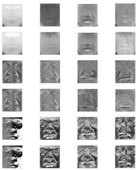
Fig. 2.The 4 principal components of`2norm PCA on depth,First row:Original data,Second

row:Corrupted data. The 4 principal components of PGA,Third row:Original data,Fourth row:Corrupted data. The 4 principal components of the proposed AAPCA,Fifth row:Original data,Sixth row:Corrupted data.

Table 1.Verification Rate for FAR=0.1% in ROC III.

Without Data Pre-processing With Data Pre-processing

Kakadiaris et al. [12] - 97.0%

Wang et al. [20] - 98.04%

AAPCA 85.0% 97.4%

`2PCA 54.2% 91.4%

PGE 68.3% 93.4%

Fig. 3.(a) The Q values obtained for all methods as a function of the number of principal com-ponents, (b) Recognition rates for all methods as a function of the percentage of occlusion.

client claims. The remaining 135 people in the database, with one image per person, are considered to be impostors. In order to produce the normal field, standard four lights PS was applied with no-preprocessing.

Since, the verification protocol offers only one image for training we applied only PCA-based algorithms. The best Equal Error Rate (EER) for all tested methods are summarized in Table 2. The proposed AAPCA achieved verification performance im-provement of more than 40%.

Table 2.EER for the Photoface database.

Methods AEP-PCA PGA AAPCA

EER 8.3% 8.1% 4.9%

5

Conclusions

References

1. S. Barsky and M. Petrou. The 4-source photometric stereo technique for three-dimensional surfaces in the presence of highlights and shadows.IEEE T-PAMI, 25(10):1239–1252, 2003. 2. S. Berretti, A. Del Bimbo, and P. Pala. 3d face recognition using isogeodesic stripes. IEEE

T-PAMI, 32(12):2162–2177, 2010.

3. V. Blanz, K. Scherbaum, and H. Seidel. Fitting a morphable model to 3d scans of faces. In

ICCV, pages 1–8, 2007.

4. K. Bowyer, K. Chang, and P. Flynn. A survey of approaches and challenges in 3d and multi-modal 3d+ 2d face recognition. CVIU, 101(1):1–15, 2006.

5. A. Bronstein, M. Bronstein, and R. Kimmel. Expression-invariant representations of faces.

IEEE T-IP, 16(1):188–197, 2007.

6. K. Chang, K. Bowyer, and P. Flynn. Multiple nose region matching for 3d face recognition under varying facial expression.IEEE T-PAMI, pages 1695–1700, 2006.

7. T. Faltemier, K. Bowyer, and P. Flynn. A region ensemble for 3-d face recognition. IEEE T-IFS, 3(1):62–73, 2008.

8. R. Fisher. Dispersion on a sphere. Proceedings of the Royal Society of London. Series A. Mathematical and Physical Sciences, 217(1130):295–305, 1953.

9. P. Fletcher, C. Lu, S. Pizer, and S. Joshi. Principal geodesic analysis for the study of nonlinear statistics of shape. IEEE T-MI, 23(8):995–1005, 2004.

10. J. Foley.Computer graphics: principles and practice. Addison-Wesley Professional, 1996. 11. B. Gokberk, H. Dutagaci, A. Ulas, L. Akarun, and B. Sankur. Representation plurality and

fusion for 3-d face recognition.IEEE T-SMCS, Part B, 38(1):155–173, 2008.

12. I. A. Kakadiaris, G. Passalis, G. Toderici, N. Murtuza, Y. Lu, N. Karampatziakis, and T. Theoharis. Recognition in the presence of facial expressions: An annotated deformable model approach.IEEE T-PAMI, 29(4):640–649, 2007.

13. W. Krzanowski. Between-groups comparison of principal components.Journal of the Amer-ican Statistical Association, pages 703–707, 1979.

14. G. Passalis, P. Perakis, T. Theoharis, and I. Kakadiaris. Using facial symmetry to handle pose variations in real-world 3d face recognition.IEEE T-PAMI, 33(10):1938 –1951, oct. 2011. 15. P. J. Phillips, P. Flynn, T. Scruggs, K. W. Bowyer, J. Chang, K. Hoffman, J. Marques, J. Min,

and W. Worek. Overview of the face recognition grand challenge. CVPR, pages 947–954, 2005.

16. C. Samir, A. Srivastava, and M. Daoudi. Three-dimensional face recognition using shapes of facial curves.IEEE T-PAMI, 28(11):1858–1863, 2006.

17. W. Smith and E. Hancock. Recovering facial shape using a statistical model of surface normal direction.IEEE T-PAMI, 28(12):1914–1930, 2006.

18. W. Smith and E. Hancock. Facial shape-from-shading and recognition using principal geodesic analysis and robust statistics. IJCV, 76(1):71–91, 2008.

19. G. Tzimiropoulos, S. Zafeiriou, and M. Pantic. Subspace learning from image gradient orientations.IEEE T-PAMI (accepted for publication), 2012.

20. Y. Wang, J. Liu, and X. Tang. Robust 3d face recognition by local shape difference boosting.