A comparative study of algorithms for automatic segmentation of dermoscopic images

A COMPARATIVE STUDY OF

ALGORITHMS FOR AUTOMATIC

SEGMENTATION OF

DERMOSCOPIC IMAGES

Bachelor’s Thesis

Cristina González Gonzalo

Bachelor’s Degree in Audiovisual System Engineering

Universidad Carlos III de Madrid

Tutor: Miguel Ángel Fernández Torres

September 2016

ii

iii

Acknowledgements

I would like to thank my parents, who have unconditionally supported me along these four years, from the very beginning until the completion of this project, during tough times with their wise advice and their encouraging words, as well as at moments of joy, with the most sincere of the smiles. Thank you for always encouraging me to keep pursuing my goals and teaching me that putting effort and passion into them leads to the best reward.

I wish to thank my sister because she is a constant source of inspiration and support. Thanks for guiding me towards and through this engineering world. She once mentioned that it is full of mountains to be climbed. Now I can say there is no better feeling than climbing them together.

I am also grateful to my family for their continuous caring, especially to my grandfather. He has never run out of words to express his support and confidence in me: “Try the best you can, because the best you can will always be good enough”.

I am thankful to the person who has changed my world and lived by my side the last two years of this immense experience. We created the perfect team to overcome bad times and celebrate the good ones.

I would like to thank my friends inside and outside this University for those shared experiences that are already meant to never be forgotten.

Finally, I would like to express my gratitude to my tutor, Miguel Ángel, for his continuous monitoring throughout the different phases of the project, as well as to the Multimedia Processing Group of Universidad Carlos III de Madrid, for their welcoming reception and giving me the chance to develop this study within their walls.

iv

Abstract

Melanoma is the most common as well as the most dangerous type of skin cancer. Nevertheless, it can be effectively treated if detected early. Dermoscopy is one of the major non-invasive imaging techniques for the diagnosis of skin lesions. The computer-aided diagnosis based on the processing of dermoscopic images aims to reduce the subjectivity and time-consuming analysis related to traditional diagnosis. The first step of automatic diagnosis is image segmentation.

In this project, the implementation and evaluation of several methods were proposed for the automatic segmentation of lesion regions in dermoscopic images, along with the corresponding implemented phases for image preprocessing and postprocessing. The developed algorithms include methods based on different state of the art techniques. The main groups of techniques which have been selected to be studied and implemented are thresholding-based methods, region-based methods, segmentation based on deformable models, as well as a new proposed approach based on the bag-of-words model. The implemented methods incorporate modifications for a better adaptation to features associated with dermoscopic images.

Each implemented method was applied to a database constituted by 724 dermoscopic images. The output of the automatic segmentation procedure for each image was compared with the corresponding manual segmentation in order to evaluate the performance. The comparison between algorithms was carried out regarding the obtained evaluation metrics.

The best results were achieved by the combination of region-based segmentation based on the multi-region adaptation of the k-means algorithm and the subsequent application of the Chan-Vese deformable model for the lesion contour refinement.

Index Terms — Dermoscopy, melanoma, automatic segmentation, skin, lesion, evaluation, comparison.

v

Index

Index of figures ... viii

Index of diagrams ... xi

Index of tables ... xii

Index of examples ... xiii

1. Introduction ... 1

1.1 Motivation and goals ... 1

1.2 Document structure ... 2

2. State of the art ... 4

2.1 Dermoscopy ... 4

2.2 Regulatory framework ... 4

2.3 Automatic segmentation techniques applied to dermoscopic images ... 5

2.3.1 Threshold-based methods ... 7 2.3.1.1 Global thresholding ... 7 2.3.1.2 Local thresholding ... 10 2.3.1.3 Multithresholding methods ... 10 2.3.2 Region-based methods ... 10 2.3.2.1 Clustering-based segmentation ... 11 2.3.3 Edge-based methods ... 12

2.3.4 Segmentation based on deformable models ... 14

2.3.4.1 Parametric deformable models ... 14

2.3.4.1.1 Traditional snakes ... 15

2.3.4.1.2 Gradient vector flow snakes ... 16

2.3.4.2 Geometric deformable models ... 19

2.3.4.2.1 Chan-Vese method ... 20

2.3.5 Segmentation based on the bag-of-words model ... 20

2.3.5.1 Detection of keypoints ... 21

2.3.5.2 Description of keypoints ... 22

2.3.5.2.1 SIFT descriptor ... 22

2.3.5.2.2 Colour-SIFT descriptors ... 23

2.3.5.3 Bag-of-words model ... 25

2.3.5.4 Adaptation to superpixel level ... 26

2.3.5.4.1 SLIC superpixels ... 26

2.3.5.4.2 Histogram intersection ... 27

2.4 Preprocessing of dermoscopic images ... 27

2.5 Postprocessing of dermoscopic images ... 28

3. System design ... 31 3.1 Problem definition ... 31 3.2 Limitations ... 31 3.3 Programming tools ... 33 3.4 Implementation ... 34 3.4.1 Preprocessing ... 34

vi

3.4.1.1 Morphological preprocessing ... 34

3.4.1.2 Filtering ... 35

3.4.2 Automatic segmentation ... 36

3.4.2.1 Threshold-based methods ... 36

3.4.2.1.1 Traditional Otsu method ... 36

3.4.2.1.2 Local Otsu method ... 38

 Local Otsu on grid ... 38

 Local Otsu on concentric rectangular partitions ... 39

3.4.2.1.3 Multithresholding Otsu method ... 40

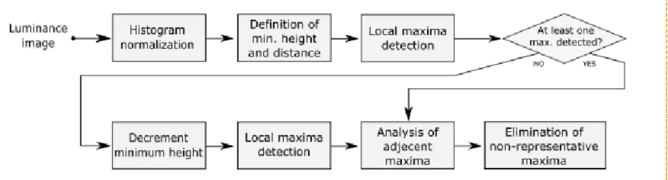
 Method to determine the number of regions within a dermoscopic image based on the analysis of local maxima in the luminance histogram... 41

3.4.2.1.4 Alternatives of design ... 43

3.4.2.2 Region-based methods... 43

3.4.2.2.1 Two-region k-means clustering ... 43

3.4.2.2.2 Multi-region k-means clustering ... 45

 Method to address illumination inconsistency in dermoscopic images ... 46

3.4.2.2.3 Alternatives of design ... 50

3.4.2.3 Segmentation based on deformable models ... 50

3.4.2.3.1 Gradient vector flow snakes ... 50

3.4.2.3.2 Chan-Vese method ... 54

3.4.2.3.3 Alternatives of design ... 55

3.4.2.4 Segmentation based on the bag-of-words model ... 57

3.4.2.4.1 Detection of keypoints ... 58

3.4.2.4.2 Description of keypoints ... 59

3.4.2.4.3 Bag-of-words model: generation of visual vocabulary ... 60

3.4.2.4.4 Matching of keypoints and visual words ... 61

3.4.2.4.5 Superpixel-level approach ... 62

3.4.2.4.6 Alternatives of design ... 64

3.4.3 Postprocessing ... 66

3.4.3.1 Morphological postprocessing ... 67

3.4.3.2 Expansion of lesion region ... 68

4. System evaluation ... 70

4.1 Database ... 70

4.2 Evaluation measures ... 70

4.3 Experiments and results ... 72

4.3.1 Threshold-based methods ... 72

4.3.1.1 Traditional Otsu method ... 72

4.3.1.2 Local Otsu method ... 75

4.3.1.3 Multithresholding Otsu method ... 76

4.3.2 Region-based methods ... 79

4.3.2.1 Two-region k-means clustering ... 79

4.3.2.1.1 Radial distance and R, G, B components ... 79

vii

4.3.2.1.3 Radial distance and S, V components ... 81

4.3.2.2 Multi-region k-means clustering ... 83

4.3.3 Segmentation based on deformable models ... 87

4.3.3.1 Gradient vector flow snakes... 87

4.3.3.2 Chan-Vese method ... 89

4.3.4 Segmentation based on the bag-of-words model ... 92

5. Conclusions ... 101

6. Future work ... 104

7. Planning and methodology ... 105

8. Socio-economic background ... 107

8.1 Budget ... 107

8.1.1 Material costs ... 107

8.1.2 Personnel costs ... 107

8.1.3 Total project cost ... 108

8.2 Socio-economic environment ... 108

References ... 110

Text references... 110

Figure references ... 114

Regulatory references ... 116

Appendix A: Further studies on state of the art ... 117

A.1 Colour spaces ... 117

A.2 Region-growing techniques ... 118

A.3 Hierarchical clustering ... 119

A.4 Edge detection operators ... 121

A.4.1 Gradient operators ... 121

A.4.2 Second derivative operators ... 121

A.4.3 Laplacian of Gaussian ... 122

A.4.4 Gaussian edge detection ... 122

A.5 Modifications of GVF algorithm ... 123

A.6 Active shape models ... 124

A.7 Modifications of SIFT descriptor ... 124

Appendix B: Cross-validation procedure ... 125

Appendix C: Summary... 126

C.1 Introduction ... 126

C.2 Preprocessing and postprocessing of dermoscopic images ... 127

C.3 Automatic segmentation of dermoscopic images ... 128

C.3.1 Threshold-based methods ... 128

C.3.2 Region-based methods ... 130

C.3.3 Segmentation based on deformable models ... 133

C.3.4 Segmentation based on the bag-of-words model ... 134

viii

Index of figures

Figure 1: Dermatoscope [I] ... 4

Figure 2: Image thresholded with Otsu method [II]... 9

Figure 3: One-dimensional edge profile [IV] ... 12

Figure 4: MR image of heart left ventricle and its potential energy function [V] ... 15

Figure 5: Effect of α on the elasticity of the curve ... 15

Figure 6: Traditional snake [VI] ... 18

Figure 7: GVF snake [VI] ... 18

Figure 8: Example of embedding a curve as a level set. From left to right: original curve, level set function where the curve is embedded as the zero level set, height map of the level set function with its zero level set in black [V] ... 20

Figure 9: Overview of method based on extraction of local features and bag-of-words model [VII] ... 21

Figure 10: SIFT keypoint descriptor [VIII] ... 23

Figure 11: Procedure adapted to colour description [IX] ... 24

Figure 12: Example of dilation [XIII] ... 29

Figure 13: Example of erosion [XIII] ... 29

Figure 14: Example of opening [XIII] ... 29

Figure 15: Example of closing [XIII] ... 30

Figure 16: Inconstant illumination [I] ... 32

Figure 17: Bubbles of fluid [I]... 32

Figure 18: Distortion [I]... 32

Figure 19: Thin hairs [XIV]... 32

Figure 20: Thick hairs [I]... 32

Figure 21: Variegated colouring [I] ... 32

Figure 22: Blood vessels [I]... 32

Figure 23: Irregular border [XIV] ...32

Figure 24: Fuzzy border [I]... 32

Figure 25: Low contrast [XIV]... 32

Figure 26: Regression [I] ... 32

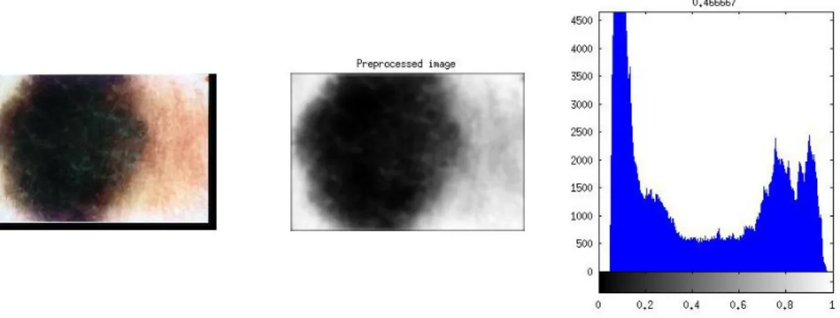
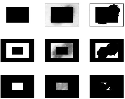
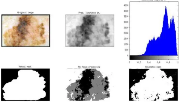
ix Figure 28: Traditional Otsu method. From left to right: original image, preprocessed luminance image, luminance histogram with threshold value situated on top (0.604). ... 37 Figure 29: Traditional Otsu method. From left to right: original image, preprocessed luminance image, luminance histogram with threshold value situated on top (0.467). ... 37 Figure 30: Pillbox and Gaussian filters [XVI] ... 38 Figure 31: Local Otsu on grid. On top: original image (left), preprocessed luminance image (center), manual mask (right). On bottom: binary mask generated by local Otsu on grid (left), mask after Gaussian filtering (center), mask after pillbox filtering (right). ... 39 Figure 32: Local Otsu on concentric partitions. From left to right: binary masks of external (top), middle (center) and inner (bottom) partitions, areas of image under each partition, thresholded partitions. ... 39 Figure 33: Local Otsu on concentric partitions. On top: original image (left) and preprocessed luminance image (right). On bottom: binary mask before (left) and after smoothing (right). ... 40 Figure 34: Multithresholding Otsu method. On top: original image (left), preprocessed luminance image (center), luminance histogram with number of required thresholds above: 3 (right). On bottom: manual mask (left), segmented regions (center), binary mask after merging of regions and complement computing (right). ... 42 Figure 35: Multi-region k-means. On top: original image (left), preprocessed luminance image (center), luminance histogram with number of determined regions above, 3 (right). On bottom: manual mask (left), mask before region merging (center), mask after region merging and complement (right). ... 46 Figure 36: Multi-region k-means. From left to right: original image, manual mask, automatic mask before image inconsistency processing ... 47 Figure 37: Multi-region k-means. On top: original image (left), preprocessed luminance image (center), luminance histogram (number of determined regions: 2) (right). On bottom: manual mask (left), mask previous to focus processing (center), automatic mask after one focus processing (right)... 49 Figure 38: Multi-region k-means. On top: original image (left), preprocessed luminance image and manual mask (center), luminance histogram (number of determined regions: 3) (right). On bottom: mask before region merging and focus processing (left), mask after first (center) and second (right) focus processing... 49 Figure 39: GVF snakes. From left to right: original image and edge map. ... 51 Figure 40: GVF snakes. Normalized gradient vector field. ... 52 Figure 41: GVF snakes. On top: horizontal and vertical components of gradient. On bottom: horizontal and vertical components of gradient vector flow. ... 52 Figure 42: GVF initial curve. Original image without black frames and initial curve on blue. .... 53

x Figure 43: Validation of internal forces parameters. Example of accuracy evolution regarding

the modification of the elasticity and rigidity parameters. ... 54

Figure 44: Chan-Vese method. From left to right: original image, multi-region k-means segmentation, Chan-Vese input mask ... 55

Figure 45: GVF snakes. Colour components analysis to define edge map. ... 56

Figure 46: Extraction of keypoints. From left to right: manual mask with Harris Laplace detected keypoints, manual mask with dense sampling detected keypoints. Lesion keypoints are shown on red and detected skin keypoints on yellow. ... 59

Figure 47: Description of keypoints. Random selection of 50 keypoints detected by Harris Laplace detector and described by SIFT descriptor. ... 60

Figure 48: Matching of keypoints and visual words. On top: original image (left) and manual mask (right). On bottom: generated binary mask after matching (left) and mask after the pillbox filter is applied (right). ... 61

Figure 49: Generation of superpixels. On top: original reference image without black frames (left), generated superpixels (center), superpixel separation between lesion and skin (right). On bottom: manual mask (left), appearance of the mask generated from superpixels division (right). ... 63

Figure 50: Detection of keypoints. From left to right: detected frames increasing from top to bottom the peak threshold (0, 10, 20, 30), detected frames increasing the edge threshold from top to bottom (3.5, 5, 7.5, 10). [XVII] ... 64

Figure 51: Variations in superpixel shape regarding the value of the regularizer parameter [XVIII]. ... 66

Figure 52: Disk-shaped structural element [XIX]... 67

Figure 53: Morphological parameters validation. Example of accuracy evolution regarding the modification of the radius of opening and closing structural elements. ... 68

Figure 54: Expansion of lesion region. ... 69

Figure 55: Representation of RGB colour space [X] ... 117

Figure 56: Representation of HSV colour space [XI] ... 117

Figure 57: Representation of Lab colour space [XII] ... 118

xi

Index of diagrams

Diagram 1: Overview of system design ... 34

Diagram 2: Preprocessing. ... 34

Diagram 3: Traditional Otsu method. ... 36

Diagram 4: Local Otsu method. ... 38

Diagram 5: Multithresholding Otsu method. Determination of number of regions in Diagram 6. ... 40

Diagram 6: Method to determine number of regions within a dermoscopic image. ... 41

Diagram 7: Two-region k-means clustering. ... 43

Diagram 8: Multi-region k-means clustering. Determination of number of regions in Diagram 6. Checking of illumination inconsistency in Diagram 9... 45

Diagram 9: Method to address illumination inconsistency in dermoscopic images. Focus analysis in Diagram 10. Focus processing in Diagram 11. ... 47

Diagram 10: Focus analysis. ... 48

Diagram 11: Focus processing. ... 48

Diagram 12: Gradient vector flow snakes. ... 51

Diagram 13: Chan-Vese method. ... 54

Diagram 14: Segmentation method based on the bag-of-words model. ... 58

Diagram 15: Superpixel-level approach. ... 62

Diagram 16: Postprocessing. ... 66

xii

Index of tables

Table 1: Evaluation concepts [XV]. ... 70

Table 2: Evaluation of traditional Otsu method. ... 75

Table 3: Evaluation of local Otsu method ... 76

Table 4: Evaluation of multithresholding Otsu method. ... 78

Table 5: Average evaluation measures for each implemented thresholding-based method. ... 78

Table 6: Evaluation of two-region k-means clustering (radial distance and R, G, B components). ... 80

Table 7: Evaluation of two-region k-means clustering (radial distance and L, a, b components). ... 81

Table 8: Evaluation of two-region k-means clustering (radial distance and S, V components). . 83

Table 9: Evaluation of multi-region k-means clustering. ... 86

Table 10: Average evaluation measures for each implemented clustering-based method. ... 87

Table 11: Evaluation of GVF snakes ... 89

Table 12: Evaluation of Chan-Vese method on B component. ... 91

Table 13: Chan-Vese method on B component and reduced points on initial curve. ... 92

Table 14: Average evaluation measures for each implemented segmentation method based on deformable models. ... 92

Table 15: Evaluation of segmentation method based on the extraction of keypoints by dense sampling, the description of keypoints by SIFT and the matching of keypoints to a vocabulary generated by k-means algorithm with 500 iterations and constituted by 32 lesion words and 32 skin words. ... 99

Table 16: Average evaluation measures for each implemented method. ... 101

Table 17: Material costs (hardware) ... 107

Table 18: Material costs (software) ... 107

Table 19: Personnel costs ... 108

xiii

Index of examples

Example 1: Traditional Otsu method. Compact lesion. From left to right: original image, manual mask, mask before postprocessing, final mask. ... 73 Example 2: Traditional Otsu method. Compact lesion with skin texture. From left to right: original image, manual mask, mask before postprocessing, final mask. ... 73 Example 3: Traditional Otsu method. Expanded lesion. From left to right: original image, manual mask, mask before postprocessing, final mask. ... 73 Example 4: Traditional Otsu method. Colour-variegated lesion. From left to right: original image, manual mask, mask before postprocessing, final mask. ... 73 Example 5: Traditional Otsu method. Lesion with inner regression areas. From left to right: original image, manual mask, mask before postprocessing, final mask. ... 73 Example 6: Traditional Otsu method. Low-contrast between lesion and skin. From left to right: original image, manual mask, mask before postprocessing, final mask. ... 74 Example 7: Traditional Otsu method. Low contrast between lesion and skin. From left to right: original image, manual mask, mask before postprocessing, final mask. ... 74 Example 8: Traditional Otsu method. Presence of hairs. From left to right: original image, manual mask, mask before postprocessing, final mask. ... 74 Example 9: Traditional Otsu method. Presence of traces of liquid. From left to right: original image, manual mask, mask before postprocessing, final mask. ... 74 Example 10: Traditional Otsu method. Illumination inconsistency. From left to right: original image, manual mask, mask before postprocessing, final mask. ... 75 Example 11: Local Otsu method. Unstable thresholds causes by skin patterns. From left to right: original image, manual mask, mask before postprocessing, final mask. ... 76 Example 12: Local Otsu method. Colour-variegated, expanded lesion. From left to right: original image, manual mask, mask before postprocessing, final mask. ... 76 Example 13: Multithresholding Otsu method. Expanded lesion. From left to right: original image, manual mask, segmented regions, final mask. ... 77 Example 14: Multithresholding Otsu method. Colour-variegated lesion. From left to right: original image, manual mask, segmented regions, final mask. ... 77 Example 15: Multithresholding Otsu method. Low contrast between lesion and skin. On top: original image (left), manual mask (center) luminance histogram (right). On bottom: segmented regions (left), final mask (right). ... 77 Example 16: Multithresholding Otsu method. Presence of liquid traces. From left to right: original image, manual mask, segmented regions, final mask. ... 78

xiv Example 17: Multithresholding Otsu method. Illumination inconsistency. From left to right: original image, manual mask, segmented regions, final mask. ... 78 Example 18: Two-region k-means clustering (radial distance, R, G, B). Low contrast between lesion and skin. From left to right: original image, manual mask, mask before postprocessing, final mask. ... 79 Example 19: Two-region k-means clustering (radial distance, R, G, B). Colour-variegated lesion. From left to right: original image, manual mask, mask before postprocessing, final mask. ... 79 Example 20: Two-region k-means clustering (radial distance, R, G, B). Illumination inconsistency. From left to right: original image, manual mask, mask before postprocessing, final mask. ... 80 Example 21: Two-region k-means clustering (radial distance, L, a, b). Low contrast between lesion and skin. From left to right: original image, manual mask, mask before postprocessing, final mask. ... 80 Example 22: Two-region k-means clustering (radial distance, L, a, b). Presence of hair. From left to right: original image, manual mask, mask before postprocessing, final mask. ... 81 Example 23: Two-region k-means clustering (radial distance, L, a, b). Colour-variegated lesion. From left to right: original image, manual mask, mask before postprocessing, final mask. ... 81 Example 24: Two-region k-means clustering (radial distance, S, V). Low contrast between lesion and skin. From left to right: original image, manual mask, mask before postprocessing, final mask. ... 82 Example 25: Two-region k-means clustering (radial distance, S, V). Presence of hair. From left to right: original image, manual mask, mask before postprocessing, final mask. ... 82 Example 26: Two--region k-means clustering (radial distance, S, V). Well-segmented, colour-variegated lesion. From left to right: original image, manual mask, mask before postprocessing, final mask. ... 82 Example 27: Two--region k-means clustering (radial distance, S, V). Poorly-segmented, colour-variegated lesion. From left to right: original image, manual mask, mask before postprocessing, final mask. ... 82 Example 28: Two--region k-means clustering (radial distance, S, V). Illumination inconsistency. From left to right: original image, manual mask, mask before postprocessing, final mask. ... 83 Example 29: Multi-region k-means clustering. Low contrast between lesion and skin. On top: original image (left), manual mask (center) luminance histogram (right). On bottom: segmented regions (left), final mask (right). ... 84 Example 30: Multi-region k-means clustering. Colour-variegated lesion. On top: original image (left), manual mask (center) luminance histogram (right). On bottom: segmented regions (left), final mask (right). ... 84

xv Example 31: Multi-region k-means clustering. Regression areas inside the lesion. On top: original image (left), manual mask (center) luminance histogram (right). On bottom: segmented regions (left), final mask (right). ... 85 Example 32: Multi-region k-means clustering. Presence of blue-white veil and traces of liquid. On top: original image (left), manual mask (center) luminance histogram (right). On bottom: segmented regions (left), final mask (right). ... 85 Example 33: Multi-region k-means clustering. Fragmented lesion. On top: original image (left), manual mask (center) luminance histogram (right). On bottom: segmented regions (left), final mask (right). ... 85 Example 34: Multi-region k-means clustering. Addressed illumination inconsistency problem. . On top: original image (left), manual mask (center) luminance histogram (right). On bottom: segmented regions (left), final mask (right). ... 86 Example 35: GVF snakes. Final curve outside the lesion region. From left to right: original image, manual mask, final mask. ... 87 Example 36: GVF snakes. Final curve inside the lesion region. From left to right: original image, manual mask, final mask. ... 88 Example 37: GVF snakes. Comparative of initial (blue) and final (red) snake, after 100 iterations. ... 88 Example 38: GVF snakes. Centered lesion that has been under-segmented. From left to right: original image, manual mask, final mask. ... 88 Example 39: GVF snakes. Expanded lesion has been under-segmented. From left to right: original image, manual mask, final mask. ... 88 Example 40: Chan-Vese method. Adjustment of final curve to real boundaries. On top: original image (left), B component (center), manual mask (right). On bottom: initial mask (left), mask before postprocessing (center), final mask (left). ... 90 Example 41: Chan-Vese method. Final contour not completely adjusted. On top: original image (left), B component (center), manual mask (right). On bottom: initial mask (left), mask before postprocessing (center), final mask (left). ... 90 Example 42: Chan-Vese method. Final contour well adjusted. On top: original image (left), B component (center), manual mask (right). On bottom: initial mask (left), mask before postprocessing (center), final mask (left). ... 91 Example 43: Harris Laplace detection at the presence of traces of liquid. ... 93 Example 44: Segmentation based on visual vocabulary and histogram intersection at superpixel-level. ... 94 Example 45: Segmentation based on dense sampling, SIFT, 32/32 vocabulary. Compact lesion. On top: original image (left), manual mask (right). On bottom: mask after matching (left), mask after filtering (center), final mask (right). ... 95

xvi Example 46: Segmentation based on dense sampling, SIFT, 32/32 vocabulary. Compact lesion that requires postprocessing to fill holes. On top: original image (left), manual mask (right). On bottom: mask after matching (left), mask after filtering (center), final mask (right). ... 95 Example 47: Segmentation based on dense sampling, SIFT, 32/32 vocabulary. Compact lesion that requires postprocessing to fill the hole inside the lesion region. On top: original image (left), manual mask (right). On bottom: mask after matching (left), mask after filtering (center), final mask (right). ... 95 Example 48: Segmentation based on dense sampling, SIFT, 32/32 vocabulary. Compact, colour-variegated lesion. On top: original image (left), manual mask (right). On bottom: mask after matching (left), mask after filtering (center), final mask (right). ... 96 Example 49: Segmentation based on dense sampling, SIFT, 32/32 vocabulary. Compact lesion with areas of low pigmentation. On top: original image (left), manual mask (right). On bottom: mask after matching (left), mask after filtering (center), final mask (right). ... 96 Example 50: Segmentation based on dense sampling, SIFT, 32/32 vocabulary. Expanded lesion. On top: original image (left), manual mask (right). On bottom: mask after matching (left), mask after filtering (center), final mask (right). ... 97 Example 51: Segmentation based on dense sampling, SIFT, 32/32 vocabulary. Low contrast between lesion and skin. On top: original image (left), manual mask (right). On bottom: mask after matching (left), mask after filtering (center), final mask (right). ... 97 Example 52: Segmentation based on dense sampling, SIFT, 32/32 vocabulary. Colour-variegated lesion. Improvement in connectivity when the number of iterations of k-means clustering is incremented. On top: original image (left), manual mask (center), mask after matching (right). On center (100 iterations): mask after filtering (left), final mask (right). On bottom (500 iterations): mask after filtering (left), final mask (right). ... 98 Example 53: Segmentation based on dense sampling, SIFT, 32/32 vocabulary. Presence of traces of liquid. Improvement in connectivity when the number of iterations of k-means clustering is incremented. On top: original image (left), manual mask (center), mask after matching (right). On center (100 iterations): mask after filtering (left), final mask (right). On bottom (500 iterations): mask after filtering (left), final mask (right). ... 99

1

1. Introduction

1.1 Motivation and goals

Melanoma is the most frequent and one of the most lethal types of skin cancer, but it is also among the most curable cancers when it is early identified. In order to improve its detection and increase survival rates for malignant melanoma, dermoscopy is integrated in the diagnosis procedure. It is a non-invasive imaging technique that allows an enhanced visualization of skin lesions, so that significant patterns that cannot be detected to the naked eye become recognisable.

Nevertheless, the traditional diagnosis procedure bases its conclusions exclusively on observation and certain visual rules regarding lesion features such as colour or asymmetry. Two main handicaps are associated with this procedure. Firstly, the diagnosis highly depends on the related complications and subjectivity of the exploration, as well as the expertise of the dermatologist. Therefore, different conclusions from the same lesion may be reached if different professionals carry out the study. Secondly, errors in diagnosis lead to the application of intrusive measures in order to surgically remove lesions wrongly classified as malignant. The computer-aided diagnosis of skin lesions aims to support conventional diagnosis and reduce its drawbacks. Regarding the first handicap, the computerized analysis of dermoscopic images provides objective and globalised diagnosis, i.e., a uniform protocol to classify the lesion as benign or malign based on a system trained through reference databases, independent of the medical center or the health professional responsible for the diagnosis. As for the second handicap, an automatic procedure allows to accurately check the presence or absence of lesion characteristics and contribute the diagnosis with an additional conclusion, which may avoid certain invasive surgical interventions such as the extraction of tissue for biopsy. Therefore, it is a time-saving technique, since it allows physicians to focus on potentially dangerous lesions while discarding harmless cases. Additionally, since the diagnosis is based on the processing of dermoscopic images taken from the patient, it facilitates remote medical treatment, which is especially beneficial in rural areas or places that are difficult to access, by means of teledermatology techniques.

The first step of automatic diagnosis is image segmentation. It supposes a phase of paramount importance because the subsequent steps are based on the accuracy of the division between lesion and skin regions. The extraction of lesion features must be applied exclusively over the lesion region in order to obtain only truly relevant characteristics to represent significant patterns related to melanoma conditions. The more exact the segmentation of the lesion region, the less the confounding information for the posterior classification algorithm.

Diverse tools and segmentation techniques are being developed over the last years in order to help the prevention of malignant melanoma. The segmentation of skin lesions is a wide field with a scattered and growing number of proposed models. In our study, different methods

2 from this broad state of the art were selected in order to be analysed, implemented and compared, along with introduced modifications and also proposed innovative techniques. This study aims to contribute to the research of optimal segmentation techniques for dermoscopic images. This area, within the automation of medical procedures, is currently under major development and progressively moving forward, since it may help cover three current healthcare necessities as previously mentioned: increase of efficiency, gratification for both involved patients and health professionals and telemedicine.

1.2 Document structure

The document is divided in different sections dedicated to specific aspects regarding our study:  Section 1: Introduction. This section presents the motivation behind the development of the project and the goals within the area of analysis as well as the objectives of the study.  Section 2: State of the art. Firstly, an overview of the dermoscopy technique and its

regulatory framework is included. Then, the section focuses on the automatic segmentation of dermoscopic images, along with the required preprocessing and postprocessing stages. An exhaustive analysis of different segmentation techniques in the specialised literature is carried out regarding their category. Several methods were selected in order to be implemented, whose formulation, functioning and application to dermoscopic images are described.

 Section 3: System design. In the first place, the problem to be solved is outlined, including the associated limitations and the programming tools that have been applied to implement the proposed solutions. Once the problem is exposed, the proposed image preprocessing and postprocessing phases as well as the implementation of the selected segmentation methods are described. For each method the corresponding introduced modifications for a better adaptation to dermoscopic images are explained. Additionally, each category of segmentation techniques includes the considered alternatives of design.  Section 4: System evaluation. In this section, the database used for the analysis of the

implemented methods is described, as well as the evaluation metrics that were chosen to evaluate the performance of the resulting segmentations. Then, the evaluation of each implemented method is presented and compared with other methods inside or outside its segmentation category, along with diverse examples of its functioning and performance statistics.

 Section 5: Conclusions. In this section, the performance of the implemented methods and several aspects regarding the obtained outcomes are interpreted. After a global comparison, the best achieved results are determined.

3  Section 6: Future work. The main segmentation factors to be improved and those lines of work that offer potential modifications are identified. Several proposed lines of investigation regarding improvement of the system are also included.

 Section 7: Planning and methodology. The main aspects related to the organization of the study development as well as the methodology of implementation are described.

 Section 8: Socio-economic background. Firstly, the budget of the project, regarding both material and personnel costs, is presented. Finally, the socio-economic environment around the study is described.

4

2. State of the art

2.1 Dermoscopy

Dermoscopy [1], also known as epiluminescence microscopy, is a non-invasive diagnostic technique based on optical magnification and either liquid immersion and low-angle-of-incidence lighting or cross-polarized lighting that allows an easy visualization of pigmented skin lesions. This diagnostic tool improves the recognition of morphological structures not visible by the naked eye or with conventional clinical images.

The technique consists in placing oil, alcohol or water on the skin lesion. This fluid eliminates surface reflection and allows a better visualization of pigmented structures within the epidermis, the dermoepidermal junction and the superficial dermis. A specific device is used for the inspection of the lesion, which is normally a dermatoscope or a digital imaging system. The magnification of these instruments range from 6x to 100x, although the widely used 10x magnification dermatoscope enables a sufficient assessment of pigmented skin lesions in daily routine [1].

Figure 1: Dermatoscope [I]

Previous studies demonstrated that dermoscopy improves accuracy in diagnosis. Dermoscopy allows the identification of numerous morphological features, such as atypical pigment networks, dots, globules, streaks, blue-white areas and blotches. This reduces screening errors and facilitates the differentiation between difficult lesions [2]. Dermoscopy is reported to have increased up to 10%-27% the sensitivity of clinical diagnosis accomplished by the naked eye [3], but it is important to take into account that formal training among dermatologists is essential for an efficient application of this technique.

2.2 Regulatory framework

In the context of dermoscopy, there are not legal requirements for the implementation of a computer-based diagnosis procedure. However, there exists a regulatory framework around the dermoscopic images obtained from patients by means of the dermoscopy technique. These are the images used by the dermatologists in order to study the primal appearance and the consequent evolution of the dermal lesions. Simultaneously, these images are employed in the implementation of automatic diagnosis systems along all the phases, including the segmentation step, studied in this project.

5 When a patient starts a dermatology treatment, pictures of his/her lesions might be required for the purpose of chronological control as a comparative measure, further study or even teledermatology service, an increasing technique for patients in rural areas. Therefore, the patient must be given a document by the dermatologist that contains all the relevant information related to the informed consent, i.e., the patient must allow the taking and storage of images and, at the same time, his/her privacy and the protection of personal data must be assured.

Regarding the taking of images, it is necessary to ensure the image rights of the patient, since an image may contain information about his/her identity and an unauthorised use may violate his/her right to privacy. The Spanish Constitution guarantees “the right to honour, to personal and family privacy and the own image” in Section 18.1 [A]. The Spanish Organic Law 1/1982 of civil protection, right to honour, to personal and family privacy and the own image, was approved according to the previous section in the Constitution [B].

The general data protection must be also secured, as the main personal data from the patient is contained within the documentation, such as name, ID number or place of residence. This aspect is regulated by the current Spanish Organic Law 15/1999 of protection of personal data [C].

The use of digital images has allowed dermatologists an easier storage and visualization of dermoscopic images. When a physician gains the patient’s informed consent, he/she is allowed to manipulate the obtained images, but has several obligations, such as encrypted storage or secured transfer of data. Additionally, if any image processing is applied to the original picture, the modifications must be stored without replacement of the initial version. Besides, dermatologists must clearly inform the patient about what the process of image manipulation involves, what the purposes are, where and for how long the images will be stored and who will have access to them [D].

2.3 Automatic segmentation techniques applied to

dermoscopic images

Image segmentation [4] is the procedure of dividing an image into multiple segments, assigning a label to every pixel, so that pixels with the same label share certain visual features, such as colour, intensity or texture. The output is a set of regions that cover the entire image. Adjacent regions are fundamentally different with respect to the same characteristics. Essentially, the main goal of segmentation is to acquire a simplified representation of an image, easier to analyse.

The standard approach in dermoscopic image analysis has three steps: 1) image segmentation, 2) feature extraction and selection, 3) lesion classification [5]. The first step of the process, i.e. the segmentation of the lesion, consists in the classification of all points in the image as part of the lesion or simply part of the surrounding non-lesional skin [6]. It is crucial for image analysis due to two main requirements. First, the border structure serves as relevant information for diagnosis, since many clinical features, such as asymmetry, border irregularity or abrupt border

6 cutoff are studied directly from the boundaries. Second, the extraction of other important clinical features, such as atypical pigment networks, globules, blue-white areas or regression structures, critically depends on the accuracy of the lesion segmentation [2].

At the clinical diagnosis of melanoma, dermatologists usually search visually for localized patterns, colours, atypical structures, as well as analysing the shape and the border of the lesion. One example of medical procedure is the ABCD rule (Asymmetry, Border, Colour and Differential structures). An alternative approach is based on the 7-point checklist and weighs the presence or absence of seven dermoscopic criteria associated with melanomas: atypical pigment network and vascular pattern, irregular streaks, dots and pigmentation, regression structures and blue-whitish veil [7].

It may be observed that this procedure is based fundamentally on the visual recognition of skin patterns and the expertise of dermatologists and may lack of objective analysis and diagnosis in some cases. Providing this diagnosis with objective measures in order to support and facilitate the dermatologists’ decisions is the main purpose of implementing an efficient automatic process for the analysis of dermoscopic images. Image segmentation, as the first step of the process, is expected to satisfy the mentioned requirements, so that the entire system can achieve an accurate diagnosis. The aim is an automatically applied segmentation phase, so that every lesion that enters the diagnosis procedure can be rapidly isolated from the non-lesional skin areas without human interaction. Therefore, time is saved for the study of the inner lesion and its boundaries are objectively defined.

Since the late 1990s numerous methods have been developed for automated segmentation of dermoscopic images. Within this project several algorithms among the main groups of techniques have been selected to be studied and applied. The following division for the selected segmentation techniques is proposed [2] [4]:

1. Threshold-based segmentation. These algorithms determine one or more proper threshold values to divide the pixels of an image into several classes and separate objects from the background.

2. Region-based segmentation. These methods segment an image into regions that are similar according to a set of predefined criteria.

3. Edge-based segmentation. These methods involve the detection of edges, important local changes in the intensity of an image, between the regions using edge operators.

4. Segmentation based on deformable models. These algorithms involve the detection of object contours using curve evolution techniques.

5. Segmentation based on the bag-of-words model. These experimental segmentation methods, already applied in the extraction of image features and image classification, are based on the detection and description of keypoints within the image and the posterior generation of a visual codebook.

Many of the methods included in this section, regardless of the segmentation techniques they are based on, take advantage of the properties that different colour spaces may offer. For instance, the implementation in one specific colour space can lead to an improvement in performance. By applying colour transformations in order to execute the same procedure in

7 different colour systems for a posterior comparison, the most suitable colour space for a particular segmentation algorithm can be found. The description of the colour spaces which have been used in our study can be found in Appendix A.1.

2.3.1 Threshold-based methods

The selection of thresholds is an important task in computer vision and detection systems. A threshold set too high may result in missed detections, while a threshold set too low may result in false positives. A fixed threshold may not perform appropriately if the properties among scenes change. Therefore, it is necessary to adapt a threshold dynamically at different scenarios in order to address these limitations [7].

Let N be the set of natural numbers, (x,y) be the spatial coordinate of a digitized image, and

G={0, 1, ... , l-1} be a set of positive integers representing gray levels. Then, an image function can be defined as the following mapping: N x N G. The gray level of a pixel with coordinate (x,y) is denoted as f(x,y). Let t ϵ G be a threshold and B = {bo, b1} be a pair of binary gray levels

and bo, b1 ϵ G. The result of thresholding an image function at gray level t is a binary image

function ft: N x N  B, such that [9]:

Regarding dermoscopic image analysis, thresholding methods achieve good results when there is defined contrast between lesion and skin, thus the corresponding image histogram is bimodal, but do not usually work accurately when the modes of two regions overlap [5].

2.3.1.1 Global thresholding

A global thresholding technique is one that thresholds the entire image with a single threshold value [9]. Within this technique two thresholding methods can be differentiated: point-dependent techniques and region-point-dependent techniques.

A thresholding method is point-dependent is the threshold is determined from the gray level of each pixel. Otsu method [10], minimum error method [11], p-tile method [9] and entropic methods [12] are among the most used techniques within this group.

On the other hand, if the threshold is determined from the local property in the neighbourhood of each pixel, then the method is region-dependent. Several methods belong to this technique, such as histogram transformation methods, methods based on second-order gray level statistics or relaxation methods [9].

This project has focused thresholding-based segmentation on point-dependent techniques, specifically the Otsu method [10], which is one of the most used threshold-based methods in

8 computer vision. It is based on unsupervised automatic threshold selection and maximizes the separability of the resultant classes in gray levels.

In ideal cases the histogram of the image has a deep and sharp valley between two of the peaks representing objects and background, so that the threshold can be set at the bottom of the valley. However, for most real pictures it is difficult to detect valley bottom precisely, especially in cases when the valley is flat and broad, there is prominent noise in the image, or the two peaks are extremely unequal in height.

Let L={1, 2, ..., L} be the number of gray levels in an image and N=n1 +n2 + nLthe total number

of pixels. The gray-level histogram is normalized and regarded as a probability distribution:

The pixels of the image are partitioned into two classes, one for the background (Co) and one

for the objects (C1), or vice versa, by a threshold k: Co denotes pixels with levels [1,...,k] and C1

denotes pixels with levels [k+1,...,L]. The probabilities of class occurrence are given by:

And the class mean levels are given by:

The zeroth- and first-order cumulative moments of the histogram up to the kth level are given, respectively, by:

While the total mean level of the original picture is:

The following relation can then verified for any value of k:

9

Let σ2Wbe the within-class or intra-class variance (the variance inside the same class), σ2Bthe

between-class variance or inter-class variance (the variance between the different classes) and

σ2T the total variance of levels. The three variances are respectively given by:

Then the following discriminant criterion measures can be determined in order to evaluate the quality of the threshold at level k, i.e., the threshold that gives the best separation of classes in gray levels:

Since η is the simplest one of the three criterion functions, it is selected as the criterion measure to evaluate the threshold. The optimal threshold k* is the one that maximizes η, or equivalently maximizes σ2B.

The maximum value, η*, can be then used as a measure to evaluate the separability of classes or the bimodality of the histogram. This is a significant measure, for it is invariant under affine transformations of the gray-level scale. It is determined within the range:

0 ≤ η* ≤ 1

10

2.3.1.2 Local thresholding

In local thresholding, the image is partitioned into smaller subimages and a threshold is computed for each subimage. The result is a thresholded image with gray level discontinuities at the boundaries of each two different subimages. A smoothing algorithm must be applied in order to reduce the discontinuities. A point-dependent method or a region-dependent method may be applied to determine the threshold of each subimage [9]. Otsu method is one of the models that can be adapted into local thresholding by dividing the original image in squares belonging to a grid that covers the entire image or concentric radial rings, and then applying the algorithm on each of those partitions.

2.3.1.3 Multithresholding methods

Many global thresholding methods can be modified in order to compute not only one threshold for the entire image, but several thresholds, so that the segmentation of different regions is more complete and exact. This is a useful tool at dermoscopic image segmentation, since most lesions contain several colour-variegated areas and a clear individual threshold at the image histogram cannot be observed. The differentiation and segmentation of each of these areas by multiple thresholds can facilitate an exact isolation of the lesion from the non-lesional skin.

Otsu method extension to multithresholding [10] is straightforward due to the discriminant criterion η. For example, in the case of three-thresholding classes segmentation, two thresholds are assumed between the minimum gray level and the maximum one (L): 1 ≤ k1< k2

< L. They separate the three classes: Co for [1, ..., k1], C1 for [k1 +1, ..., k2], and C2 for [k2 +1, ...,

L]. The criterion measure η, equivalent to σ2

B, is then a function of two variables (k1and k2) and

two optimal thresholds (k1* and k2*) are determined by maximizing σ2B:

The selected thresholds generally become less conclusive when the number of classes o be separated increases. This is because the criterion measure, σ2B, has been defined in

one-dimensional scale and may lose its meaning as the number of classes is incremented. It should also be noticed that the expression of σ2B and the maximization procedure become more

complex.

2.3.2 Region-based methods

Region-based methods involve the distribution of pixels into several homogenous regions according to common image properties [13], which consist of:

- Intensity values from the original image or computed values based on image operators.

- Textures or patterns that are exclusive to each type of region. - Spectral profiles that provide multidimensional image data.

11 Region-based methods can facilitate the segmentation of those dermoscopic images in which lesions contain several areas with different colour and texture, since every region can be segmented separately and merged together afterwards. Nevertheless, these approaches can have difficulties in these cases too, that is, when the lesion as well as the skin region are too textured or have colour-variegated areas, leading to an oversegmentation problem, where an exceeding number of subregions are detected and the merging processing becomes more complicated.

There exist two fundamental types of region-based segmentation techniques: clustering-based segmentation and region-growing techniques. The region-based algorithms implemented in this project are based on clustering-based segmentation. Therefore, a deeper analysis of these methods is included in the next section. Nevertheless, in Appendix A.2 an overview of region-growing techniques can be found.

2.3.2.1 Clustering-based segmentation

A cluster is a collection of objects which are similar among them and are dissimilar to the objects that belong to other clusters. Therefore, the goal of clustering-based methods is to determine the intrinsic grouping in a set of unlabeled data [14]. Clustering problems are present in many different applications, such as vector quantization and pattern recognition. The approach of what constitutes a good cluster depends on the application and there are many methods for finding clusters according to various criteria [15].

Clustering techniques can be divided into two categories: partitional clustering and hierarchical clustering. Partitional clustering segmentation approaches have been the ones selected for implementation in this project and they are described below. However, an overview of the application of hierarchical clustering is included in Appendix A.3.

Partitional clustering decomposes a data set into a set of disjoint clusters. Given a data set of N

points, a partitioning method creates K (N ≥ K) partitions of the data, with each partition representing a cluster, by satisfying the following requirements [16]:

1) Each group contains at least one point.

2) Each point belongs to exactly one group, although in fuzzy partitioning methods, which are not covered in this project, a point can belong to more than one group.

Many partitional clustering formulations attempt to minimize an objective function. Among these formulations the most widely used is k-means clustering, which is covered in our study. Given a set on n data points in real d-dimensional space, Rd, and an integer c, the aim of the algorithm is to determine a set of c points in Rd, so that the distance from each data point to its nearest center is minimized [15], i.e., a squared error function is minimized:

where ||xi – vj|| is the Euclidean distance between a data point and the cluster center, ciis the

12 The minimization of the objective function is carried out by an iterative procedure that comprises the following steps [13]:

1. A number of c points are placed into the space represented by the objects that are being clustered. These points are the initial group of centroids.

2. Each object is assigned to the group with the closest centroid.

3. When all objects have been assigned a centroid, the positions of the c centroids are recalculated.

4. The steps 2 and 3 are repeated until the centroids do not change their position, i.e., until a convergence condition is reached. The algorithm will eventually converge to a point that is a local minimum, but the result does not have to be necessarily a global minimum [15].

K-means clustering process may be hindered by image noise and outliers with the data, but it is relatively robust, fast and efficient. It requires a priori specification of the number of clusters, that is, it is necessary to introduce the number of final regions into which the objects will be grouped. This can be tricky when it comes to dermoscopic image segmentation, as every lesion can have its own pattern for the number of differential lesional areas. The algorithm is also significantly sensitive to a random initialization of the centroids. In dermoscopic images it is important to determine certain fixed initialization for the centroids, so that the process of separating lesion and skin areas can be facilitated from the beginning and the clusters are created taking into account these initial features.

2.3.3 Edge-based methods

Edge-based segmentation is based on edge detection algorithms, whose aim is to identify those points in the image where there are discontinuities in brightness in order to find the boundaries of objects within the image.

Discontinuities in image intensity can be either step discontinuities, where the image intensity abruptly changes from one value on one side of the discontinuity to a different value on the opposite side, or line discontinuities, where the image intensity abruptly changes its value but returns to the starting value within short distance. However, these types of sharp borders are rare in real images because of low-frequency components and the smoothing of sensing devices: step edges become ramp edges and line edges become roof edges [21].

13 It is difficult to develop an edge detection operator that reliably finds edges and is immune to noise. Several steps are necessary in order to achieve an accurate detection [21]:

1. Filtering: since some edge detection algorithms are susceptible to noise and other handicaps in discrete computations, a filter is commonly applied to improve their performance. However, there must be a trade-off between edge strength and noise reduction. If the level of accuracy is too high, noise will cause the detection of numerous false edges. On the other hand, if too much filtering is applied to the reduction of noise, the accuracy might be reduced because many relevant edges might not be detected [19].

2. Enhancement: the detection of edges is facilitated by determining changes of intensity in the neighbourhood of a point. Enhancement emphasizes pixels where there is a significant local change of intensity and is usually performed by computing the gradient magnitude.

3. Detection: many points in an image satisfy the criteria to be considered as part of an edge, but only those points with strong edge content are desired. Some method should be used to determine which points are edge points. Frequently, thresholding provides the criterion used for detection.

Many edge detection algorithms include a fourth step:

4. Localization: the location of the edge and its orientation can be estimated with subpixel resolution if required.

Some of the most used edge detection operators are classified and described in Appendix A.4. The description of each detector is based on the exhaustive analysis included in [21].

Dermoscopic image segmentation presents a set of difficulties to edge-based methods due to their criteria of detection. Edge-based approaches perform poorly when the boundaries of the lesion are not well defined and the transition between skin and lesion is smooth. In these situations the resultant edges contain gaps and the contour of the lesion may leak through them. Another difficulty for these methods is the presence in the image of some elements such as hair, specular reflections and irregularities in the skin texture. In these cases it is common the appearance of spurious edge points that do not belong to the lesion boundary [5].

Although some edge-based techniques present advanced implementations that aim to resolve some handicaps of these algorithms, such as the sensitivity to noise and the selection of a unique, fixed threshold, the edge detectors are still affected by the properties of dermoscopic images. For this reason, they are usually combined with other more specific and developed methods, which exploit the advantages of edge-based algorithms and include them as a phase of the entire procedure. It is the case of the traditional active contours model, which is studied in the next section.

14

2.3.4 Segmentation based on deformable models

Deformable models, also referred to as snakes or active contours, are curves or surfaces defined within an image domain that can move under the influence of internal forces, which are defined within the curve or surface itself, and external forces, which are computed from the image data. The internal forces keep the model smooth during the deformation process, whereas the external forces move the model toward an object boundary or other desired features within the image. By constraining extracted boundaries to be smooth and incorporating a priori information about the shape of the object to be segmented, deformable models allow integrating boundary elements into a consistent mathematical description [22]. Active contour algorithms are often very sensitive to initialization. The initial snake points can be manually defined by an operator or automatically determined. In order to make the segmentation process fully automated, an effective automatic snake initialization method is required [23].

There are two types of deformable models: parametric deformable models and geometric deformable models.

2.3.4.1 Parametric deformable models

Parametric deformable models represent curves explicitly in their parametric forms during deformation. This representation allows direct interaction with the model and can lead to a compact representation for fast real-time implementation [22]. Parametric active contours synthesize parametric curves within an image domain and allow them to move toward desired features, usually edges [24].

There are two different types of formulations for parametric deformable models: energy minimization formulation and dynamic force formulation. The two formulations lead to similar results, but the first one has the advantage that its solution satisfies a minimum principle, whereas the second one has the flexibility of allowing the use of more general types of external forces [22]. The parametric deformable models studied in this project are based on the energy minimization formulation.

The premise of the energy minimization formulation is to find a parameterized curve that minimizes the weighted sum of internal energy and potential energy. The internal energy specifies the tension or the smoothness of the contour. The potential energy is defined over the image domain and typically has local minima at image intensity edges occurring at object boundaries, which can be observed in the following figure [22].

15

Figure 4: MR image of heart left ventricle and its potential energy function [V]

Typically, the curves are drawn toward the edges by potential forces. Additional forces, such as pressure forces or gradient vector flow, which is studied later, comprise the external forces. There are also internal forces designed to hold the curve together (elasticity forces) and to keep it from bending too much (bending forces) [24]. In order to find the object boundary, parametric curves are initialized within the image domain and are forced to move toward the potential energy minima under the influence of both of these forces [22].

2.3.4.1.1 Traditional snakes

As described in [24], a traditional snake is a curve x(s) = [x(s), y(s)], s ϵ [0, 1], that moves through the spatial domain of an image to minimize the following energy functional:

where x’(s) and x’’(s) denote the first and second derivatives of x(s) with respect to s. The parameters α and β are weighting parameters that control the tension and the rigidity of the snake, respectively: α controls the penalty for internal elasticity and bigger values mean less stretching; bigger values of β mean the curve is harder to bend (if β=0 the snake becomes second order discontinuous and develops a corner).

Figure 5: Effect of α on the elasticity of the curve

The external energy function Eext is derived from the image so that it reaches its smaller values

at the features of interest, such as boundaries. Given a gray-level image I(x,y), typical external energies designed to lead an active contour toward step edges are:

16 where Gσ(x,y) is a two-dimensional Gaussian function with standard deviation σ and ∇ is the

gradient operator. Larger values of σ will cause the boundaries to become blurry, but they are sometimes necessary in order to increase the capture range of the active contour.

A snake that minimizes E must satisfy the following Euler equation:

This can be interpreted as a force balance equation:

The internal force Fint controls the stretching and bending and the external potential force

Fext(p) pulls the snake toward the desired image edges.

To find a solution to the Euler equation, the snake is made dynamic by treating x as function of time t as well as s and computing iteratively until it stabilizes and a numerical solution is achieved.

A key problem with traditional snake formulation is its limited capture range. The magnitude of the external forces decreases rapidly away from the object boundary. As a consequence, the initialization of the contour must be close to the original boundary or else it likely converges to the wrong result. Additionally, prior knowledge of whether to shrink or expand the snake is needed. When σ is increased the range is augmented, but the boundary localization becomes less accurate and distinct. Traditional snakes also show difficulties at adapting to boundary concavities.

2.3.4.1.2 Gradient vector flow snakes

The analysis included in [24] describes the gradient vector flow (GVF) as a class of external forces. These forces are dense vector fields derived from images by minimizing a certain energy functional in a variational framework. The minimization is achieved by solving a pair of decoupled linear partial differential equations that diffuses the gradient of an edge map in regions distant from the boundary. The amount of diffusion adapts according to the strength of the edges to avoid the distortion of object boundaries [22].

GVF snakes have advantages over traditional snakes. They are less sensitive to initialization and have the ability to move into boundary concavities. Besides, a GVF snake does not require prior knowledge whether to shrink or expand toward the boundary. These snakes also have a larger capture range, so the curve can be initialised farther away from the boundary.

The previously computed force balance condition is used as starting point:

17 The first step is the definition of an edge map f(x, y), derived from the image I(x, y), having the property of being larger near the image edges. Any gray-level or binary edge map can be used, for example:

The edge map satisfies three general properties. First, the gradient of an edge map (∇f) has vectors pointing toward the edges, which are normal to the edges at the edges points. Second, these vectors have normally large magnitudes only in the vicinity of the edges. Third, in homogeneous regions, where I(x, y) is nearly constant, ∇f is nearly null.

These properties have consequences on the behaviour of a traditional snake. The first one is a highly desirable property, since a snake initialized close to the edge will converge to a stable configuration near the edge. But the second and the third properties are undesirable. Because of the second property, the capture range will be very small, and homogeneous regions will have no external forces due to the third property. The GVF snakes aim to keep the desirable property of the gradients near the edges and at the same time extend the gradient map farther away from the edges and into homogeneous regions using a computational diffusion process. This way, the snake will be able to move toward object boundaries and boundary concavities even from homogeneous regions.

A new static external force, the gradient vector flow (GVF) is then defined: Fext(g) = v(x, y) = [u(x,

y), v(x, y)]. It minimizes the following energy functional:

When ∇f is small, the energy is dominated by the sum of the squares of the partial derivatives of the vector field, yielding a slow varying field, i.e., the result is smooth in the absence of data. When ∇f is large, the second term dominates the integrand and is minimized by setting v = ∇f. Therefore, v is kept nearly equal to the gradient of the edge map when it is large, but the field is forced to be slowly-varying in homogeneous regions.

The parameter μ regularizes the trade-off between the first and the second term of the integrand. It should be set according to the amount of noise present in the image: it should be increased when there is a high amount of noise.

To