Technische Universität München Lehrstuhl für Mathematische Optimierung
Adaptive Numerical Solution of State Constrained
Optimal Control Problems
Olaf Benedix
Vollständiger Abdruck der von der Fakultät für Mathematik der Technischen Universität München zur Erlangung des akademischen Grades eines
Doktors der Naturwissenschaften (Dr. rer. nat.) genehmigten Dissertation.
Vorsitzender: Univ.-Prof. Dr. Peter Rentrop Prüfer der Dissertation: 1. Univ.-Prof. Dr. Boris Vexler
2. Univ.-Prof. Dr. Thomas Apel
(Universität der Bundeswehr München)
Die Dissertation wurde am 14. 06. 2011 bei der Technischen Universität München eingereicht und durch die Fakultät für Mathematik am 11. 07. 2011 angenommen.
Contents
1. Introduction 1
2. Basic Concepts in Optimal Control 7
2.1. Problem setting . . . 7
2.1.1. Notation . . . 7
2.1.2. State equation . . . 8
2.1.3. State constraints . . . 12
2.1.4. Cost functional . . . 15
2.2. Existence and uniqueness of optimal solutions . . . 16
2.3. Discretization and optimization algorithms for problems without pointwise constraints . . . 18
2.3.1. Optimality conditions . . . 18
2.3.2. Evaluation of derivatives . . . 20
2.3.3. Discretization . . . 22
2.3.4. Optimization methods for unconstrained problems . . . 24
2.4. Treatment of inequality constraints . . . 27
2.5. A posteriori error estimation and adaptive algorithm . . . 30
3. Elliptic Optimal Control Problems with State Constraints 35 3.1. Analysis of the state equation . . . 35
3.2. Optimality conditions . . . 38
3.3. Finite element discretization . . . 41
3.3.1. Discretization of the state variable . . . 41
3.3.2. Discretization of Lagrange multiplier and state constraint . . . 44
3.3.3. Discretization of the control variable . . . 45
3.3.4. Discrete optimality conditions . . . 46
3.4. Optimization with the primal-dual active set method . . . 47
3.5. A posteriori error estimator and adaptivity . . . 52
3.6. Regularization and interior point method . . . 58
4. Parabolic Optimal Control Problems with State Constraints 61 4.1. Continous setting and optimality conditions . . . 61
4.2. Regularization . . . 64
4.3. Finite element discretization in space and time . . . 65
4.4. Optimization by interior point method . . . 68
4.5. A posteriori error estimator and adaptivity . . . 70
5.1. Complete algorithm . . . 79
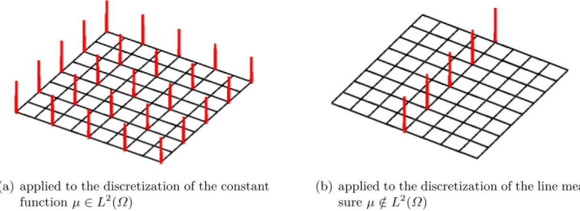
5.2. Implementation of Borel measures . . . 81
5.3. Possible modifications of the standard algorithm . . . 83
5.4. Considerations derived from practical problems . . . 85
6. Numerical Results 89 6.1. Elliptic problem with known exact solution . . . 90
6.2. Elliptic problem with unknown exact solution . . . 94
6.3. Nonlinear elliptic problem . . . 96
6.4. Parabolic problem . . . 98
7. Optimal Control of Young Concrete Thermo-Mechanical Properties 103 7.1. Problem introduction . . . 103
7.2. Modelling the involved quantities . . . 104
7.3. State equation . . . 110
7.4. Optimization problems . . . 115
7.4.1. State constraint . . . 116
7.4.2. Cost functional . . . 117
7.5. Examples and numerical results . . . 118
7.5.1. Control of initial temperature and heat transfer . . . 118
7.5.2. Control of the concrete recipe . . . 122
7.5.3. Control of the flow rate of a water cooling system . . . 124
8. Summary 129
Acknowledgments 131
A. Convergence order for the Laplace equation with irregular data 133 B. Utilized data for the models of the material properties of concrete 143
List of Figures 145
List of Tables 147
List of Algorithms 149
1. Introduction
The central subject of interest of this thesis is the class of optimal control problems with partial differential equations and additional state constraints. The focus lies especially on the construction of numerical solution algorithms to find an approximate solution to such a problem, and the effectiveness of such algorithms.
The central problem class features many different ingredients, over which we give a short overview here. The general problem form considered is
(P) minJ(q, u) q∈Q, u∈X u=S(q) G(u)≥0 . (1.1)
Here,uis called thestate function, searched for in thestate spaceX, andq thecontrol variable, searched for in the control spaceQ. In the field of optimal control, X is usually considered a function space. The domain of the state functions might be a spatial domain Ω ⊂ Rn
(n∈ {2,3}) or in the case of time-dependent problems a domain in time and spaceI×Ωwith a given time intervalI = (0, T). The operatorS is calledcontrol-to-state operator. It represents the solution operator of a partial differential equation, which in turn is called thestate equation. In this thesis, elliptic and parabolic state equations are considered. The problem (P) is then called elliptic, or parabolic optimal control problem (OCP), respectively. The functional J:Q×X→Ris called the cost functional, and the functionG is theconstraint function for the state. With all these ingredients present, (P) is called astate constrained optimal control problem. Without the condition G(u)≥0 one would speak of an unconstrained optimal control problem, which can be regarded as the basis class of optimal control problems.
Unconstrained optimal control problems have been of interest in applied mathematics for some time now. A lot of practical problems, their origin ranging from civil engineering via optics to chemical engineering and biological applications, can be modeled as optimal control problems with partial differential equations. This is not surprising, since most technical processes allow for user input after the initial setup, and guiding the system’s output to a user-determined configuration is a natural desire as well. Also understandable is the possible need for bounds on input and output variables. For most technical problems, only certain amounts of input are possible, and concerning the output, certain states might lead to catastrophic scenarios that must be avoided at all cost.
This thesis deals with state constrained problems, which can be motivated in different ways. From the viewpoint of the field of optimization, (P) can be seen as an optimization problem on Q×X, with a partial differential equation as an equality constraint, and a pointwise inequality constraint. The motivation to consider this problem class becomes possibly clearer from an applicational point of view. Suppose that a scientific or technical process of interest
is described by a partial differential equation. For notational purposes the quantities which are considered influencable are gathered in the control variable q. On the other hand, the quantities that are regarded as descriptive of the process’ status, are gathered in the state functionu. We think of the partial differential equation in such a way thatu is the solution depending on q, and thus write formallyu =S(q). The quest is now to find the pair (q, u) of a control q and corresponding stateu =S(q) that is the most favorable to the user. By means of the conditionG(u)≥0 with a properly modeled function Gthe user can rule out some pairs completely. Amongst the remaining pairs, favorability is determined by a given functionalJ(q, u). This functional is modeled in such a way that a more favourable pair (q, u) is mapped to a smaller value of J.
Optimal control problems with partial differential equations have been subject of investigation for some time, see [63] for an early main work considering elliptic, parabolic and hyperbolic optimal control problems. Numerical methods to solve these OCPs are usually comprised of two steps, a discretization by the finite element method, and the solution of a discrete optimal control problem. These steps are connected in an overall algorithm, so that a more or less sophisticated sustained refinement of the discretization in the former step leads to optimal solutions in the latter step which converge to the solution of the continous problem (P). For elliptic OCPs without additional constraints solution methods have been discussed in [32, 38] and many following publications. A priori discretization error estimations have been derived for a number of settings and discretization methods. The most basic result considers a distributed linear-quadratic optimal control problem on a convex domain of computation. By using discretizations with linear finite elements described by uniform meshes withdiscretization parameter h, the order of convergence of the finite element solutions qh to the exact one
can be proven to be h2 in the L2-norm if either the variational discretization concept or a postprocessing step is used, see [51, 71].
Parabolic problems pose more difficulties even for proving the existence of optimal solutions, see [35, 63, 92]. Solution techniques have been developed and for the most basic case of distributed control,Q=L2(I×Ω), the linear-quadratic optimal control problem discretized by linear finite elements in space, uniform with discretization parameterh, and the dG(0)-method in time, uniform with discretization parameter k, the convergence order of h2+khas been established for the controls qkh to q in the L2-norm. A proof can be found in [67], as a special
case of a more general result allowing for finite elements of different order.
A neighboring problem class frequently under consideration is the class of control constrained optimal control problems. Here it is the control q that is required to fulfill the pointwise constraint,G(q)≥0, rather than the state u. The presence of this additional constraint may reduce the regularity of the optimal solution of the OCP. This, in turn, reduces the order of convergence of the numerical solution. An overview over different situations can be found in [64]. A counter-measure to speed up the performance, or even restore the full convergence order is the construction of locally refined meshes, that take the structure of the problem into account. A widely used approach is the use of adaptive methods, where the discretization error is estimated a posteriori on a coarse starting grid, and expressed in local contributions. By the principle of equilibrating these error contributions, a local refinement algorithm is set up. One example, where the a posteriori estimation assesses the error in the natural norms of the involved spaces, can be found in, e.g., [46, 62]. A different approach is calledgoal oriented
adaptivity, here the error in terms of a functional of interest, for example the cost functional, is estimated, see, e.g., [94].
In the problem class (1.1) that is in this thesis’ center of attention, major care has to be put on the state constraint. In comparison to unconstrained optimal control problems, the introduction of the state constraint has the direct effect of a reduced regularity of the optimal solution, see, e.g., [17]. This has further consequences for the construction of solution algorithms for (1.1). Consider first the solution of one discretized optimal control problem only. A direct approach, yielding exploitable optimality conditions by incorporating the state constraint by the Lagrange formalism, shows that the Lagrange multiplier, denoted by µh, is in general a regular Borel
measure. This means that a direct numerical treatment of this problem needs to face the handling of Borel measures, and a simple transfer of the methods for unconstrained optimal control problems is not possible. The method of choice to solve the discretized OCPs will be a primal-dual active set method, introduced in [14].
An alternative approach is the regularization of the problem (P) on the continous level. This means the construction of problems (Pγ), with γ ∈ R being the regularization parameter,
whose solution exhibits the higher regularity, but is close to the original solution in the sense that the regularized solutions converge to the original solution withγ → ∞. These regularized problems can subsequently be numerically solved with methods for unconstrained OCPs. This approach leaves the question of how to balance the driving ofγ → ∞ andh→0 (and possibly k→0) to achieve maximum effectivity of the method. Concrete choices of regularization are the Moreau-Yosida-regularization, see [49, 54], and barrier methods, see [85, 86]. In this thesis, the latter method is investigated.
Apart from the optimization on one discretization level, consider now the process of refinement of the discretization. A second consequence of the reduced regularity is again the reduction of the achievable order of convergence of the discretization error in terms of h → 0, k→ 0 if uniform discretization is used, see, e.g., [26, 69]. Thus it is desirable to set up a mesh refinement strategy to improve the convergence. In this thesis, a goal-oriented a posteriori error estimator is derived by the dual weighted residual method, see [7] for an overview. For problem (1.1) the error estimator is dissected into the contributions, if they are present,
η:=ηh+ηk+ηd+ηγ, (1.2)
which are the spatial discretization error, temporal discretization error, control discretization error, and regularization error. Each of these contributions is then further split up into cellweise or intervall-wise contributions, where applicable. The so obtained error indicators are used in the execution of the mesh refinement strategy. In the construction of a comprehensive solution algorithm for state constrained optimal control problems one must be aware that regularities and convergence orders can also be reduced due to other phenomena, for example boundary properties like reentrant corners or edges, or nonsmooth boundaries, or singularities in the data, like jumping coefficients. If the spatial location of these singularities is known, they can be treated with a priori knowledge, e.g. mesh grading techniques, see, e.g., [89] and the references therein. The spatial location of the singularities due to the state constraints however is a priori unknown. Therefore it is advantageous to use a posteriori techniques.
An additional goal of investigation in this thesis is the treatment of a large-scale real-world problem, which originates from the field of civil engineering. For structures made of concrete,
the time span of the first few days after the concrete pour is called young concrete phase. During that phase the concrete solidifies, and its thermomechanical properties develop. Amongst others, tensile strength is built up with time. The exact progression depends on the temperature field inside the structure, which is changing due to chemically produced heat and heat outflow. These phenomena in turn depend on initial and boundary conditions and material parameters. Counteracting to this tensile strength, tensile stresses are building up. Should at any point the tensile stress exceed the strength, the concrete will crack, which is seen as an event that is to be avoided. The goal is to choose boundary conditions and material in such a way that no cracks occur.
This practical problem can be modeled as an optimal control problem. The prohibition of cracks translates as a constraint on the state variable. The state equation is a parabolic equation coupled with one ordinary differential equation in every spatial point. So the problem does not fit in the category (1.1) strictly speaking, but on the other hand the additional ordinary differential equation can be treated by standard methods. Since the concrete structures are generally large-scale and nonconvex, a goal-oriented discretization is required. Thus the numerical treatment of this problem by the methods developed in this thesis assures the necessary effectivity.
Summarizing, the goal of the thesis is the efficient numerical solution of optimal control problems with elliptic or parabolic state equation and pointwise state constraints, with all aspects mentioned above to be taken into consideration. Preferably large problem classes are set up. The two numerical solution strategies, amounting to the primal-dual active set strategy and to an interior-point method, are developed for a given discretization. For both these strategies a posteriori error estimators are derived, and used to guide an adaptive mesh refinement algorithm.
The thesis is divided into the following chapters:
In Chapter 2 the necessary basic notation is introduced, as well as the basic form of elliptic and parabolic state constrained optimal control problems. This includes the general formulation of elliptic and parabolic state equations, state constraints and cost functionals. Assumptions that allow for the proof of existence and uniqueness of optimal solutions are given. Common concepts of numerical solution strategies are introduced: for unconstrained optimal control problems the process of deriving optimality conditions, discretization and optimization meth-ods are described, serving as a starting point for the development of the equivalent steps in the treatment of state constrained problems. An overview of methods to include the state constraints is then given, and the strategy for a posteriori error estimation and the adaptive mesh-refinement algorithm is laid out.
In Chapter 3, these general concepts are concretized for elliptic optimal control problems with state constraints. The state equation is formulated in a precise setting. For a large problem class the unique existence of optimal solutions is proven. Necessary optimality conditions of first order are given. The finite element discretization is described in detail, a continous Galerkin method of ordersis used to discretize the state space. For this discretized problem the optimization is carried out with the primal-dual active set method. The a posteriori error estimator is derived, consisting of the spatial part ηh and the control discretization part ηd.
With subsequent splitting into the respective cellwise error indicators, the adaptive mesh refinement algorithm is set up. Finally the interior point method as alternate optimization method is introduced briefly.
Chapter 4 deals with parabolic state constrained optimal control problems. Giving a precise setting again allows to prove existence of an optimal solution and necessary optimality condi-tions for it. The regularization by barrier funccondi-tions is introduced, and optimality condicondi-tions of the regularized problem are derived. Further, the finite element discretization in space and time is carried out, using a continous Galerkin method of order sin space as before, and the discontinous Galerkin method in time. The interior point optimization algorithm is applied. The a posteriori error estimator derived distinguishes between the influences of regularization, ηγ, and temporal, ηk, spatial, ηh, and control discretization, ηd. Implementational aspects
are considered in Chapter 5. A combination of all ingredients to a comprehensive solution algorithm is given, considerations on the choice of parameters are made. Improvements of subalgorithms in special situations are discussed.
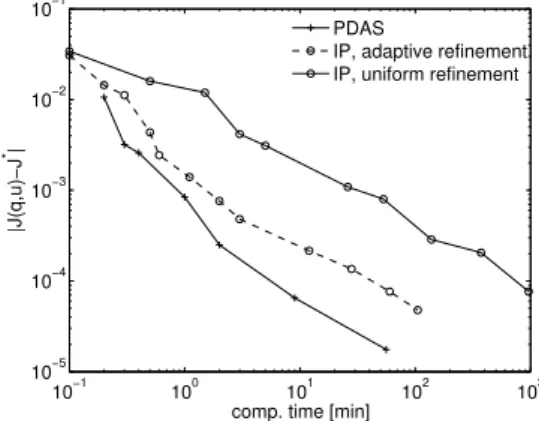
Numerical experiments to validate the theoretical results and the advised optimization algo-rithms of this thesis are carried out in Chapter 6. Combinations of elliptic and parabolic, linear and nonlinear test problems with different structures of the active set are considered. The efficiency of the error estimator itself, and its parts ηγ, ηk, ηh, ηd is evaluated. Also the
adaptive refinement strategy driven by the local error indicators is compared to the uniform refinement strategy by the respective convergence rates.
Chapter 7 contains the application of the methods discussed in this thesis to the real-world application of optimal control of young concrete thermo-mechanical properties. The model functions for the different physical phenomena are introduced and the possibilities how to assemble an optimal control problem are shown. The unique solvability of the state equation and the existence of an optimal control is proven. Finally, several numerical examples are considered and solved by the methods developed in this thesis.
2. Basic Concepts in Optimal Control
2.1. Problem setting
2.1.1. Notation
In the following, we will introduce the basic notation used throughout the thesis, and describe the considered problem class in a rather abstract formulation. Let Ω⊂Rn, n∈ {2,3}denote a
spatial domain with Lipschitz boundary∂Ω =:Γ. For a pointx∈Γ letn(x) denote the outer unit normal vector ofΩ, if it exists. ByLp(Ω),Wm,p(Ω), and Hm(Ω) with 1≤p≤ ∞, m∈R
we denote the usual Lebesgue and Sobolev spaces. The space of continous functions on ¯Ω with continous derivatives up tom-th order,m= 0,1, . . . is denoted byCm( ¯Ω), and the dual space toC0( ¯Ω) =C( ¯Ω) is identified with the space of regular Borel measures M(Ω).
The considered time interval is denoted by I = (0, T) ⊂ R. For any Banach space Z and time interval [t1, t2] the Lebesgue and Sobolev spaces of time dependent, Z-valued functions are denoted byLp([t1, t2], Z), Wm,p([t1, t2], Z), Hm([t1, t2], Z). For a proper definition of these spaces including Bochner integrals, see, e. g., [99]. If [t1, t2] =I, the interval can be omitted in the previous notation, and we just write Lp(Z), Wm,p(Z), Hm(Z). Again we identify C( ¯I×Ω)¯ ∗ = M(I ×Ω). The following convention concerning the evaluation of space and time dependent functions is used: a functionv∈C(I×Ω) can be interpreted as an abstract function v: [0, T]→C(Ω), so that it is possible to write both v(t, x) (a number) and v(t) (a C(Ω)-function) without being ambiguous.
All function spaces can be endowed with a subscript to prescribe a homogenous Dirichlet boundary condition; the subscript 0 indicates the boundary condition is prescribed on the whole boundary. If the condition is to be applied to a partΓ1⊂Γ only, the subscriptΓ1 is used.
LetV, H, R be Hilbert spaces equipped with scalar products (·,·)V, (·,·)H, and (·,·)R,
respec-tively, such thatV is continously and densely embedded into H. With the dual spacesV∗ and H∗ the Gelfand tripleV ,→H ,→ V∗ is formed, assuming an identification of H with H∗ is possible. This makes it possible to represent functionals inV∗ with their effect in the duality pairingh·,·iV∗,V by the effect in inner products (·,·)H. Abbreviations for the most commonly used scalar and duality products are
(., .) := (., .)H, (v, w)I:= Z I (v(t), w(t))Hdt, v, w∈L2(I, H), (·,·)Ω:= (·,·)L2(Ω), (·,·)I×Ω := (·,·)L2(I×Ω), (·,·)Γ := (·,·)L2(Γ), (·,·)I×Γ := (·,·)L2(I×Γ), h·,·i:=h·,·iM(Ω),C( ¯Ω), h·,·iI :=h·,·iM(I×Ω),C( ¯I×Ω¯).
Throughout this thesis, parlance and notation will be differentiated depending on the type of state equationS represents. The first case considers stationary problems, where the state equation is an elliptic partial differential equation. After the general introduction in this section, Chapter 3 is devoted to the study of elliptic optimal control problems with state constraints. Here, the domain of the state functions u∈X is ¯Ω. The specific choice of the state space X is done in Chapter 3, as it depends on the properties of (1.1). However, one basic regularity requirement that needs to be fulfilled simply because of the presence of the pointwise state constraints, is the continuity of the states on the whole domain. This property is used as a starting point for the derivation of optimality conditions, see [92, section 6.1], as it assures that the cone of non-negative functions has interior points. Thus we require
X ⊂C( ¯Ω) for elliptic OCPs. (2.1)
As a second case, time-dependent problems are considered, with the state equation being of parabolic type. The detailed treatment is done in Chapter 4. As the state is now time and space dependent, the domain of the state functionsu∈X is ¯I×Ω. Including the continuity of¯ the state function on the computational space-time domain, the state space has to be chosen according to
X⊂C( ¯I×Ω)¯ for parabolic OCPs. (2.2) For the choice of the control space no additional regularity requirements are made. The domain of the control functions q∈Qis a subset of ¯Ω for elliptic optimal control problems, and a subset of ¯I ×Ω¯ for parabolic optimal control problems. The actual choice depends on the problem structure, specifically the way in whichq enters the state equation. In the case of parameter control, it is also possible to choose Q⊂Rk or Q⊂L2(Rk) as a subspace,
respectively.
2.1.2. State equation
The state equation is frequently introduced in different formulations. The classical form employs a differential operator that will be denoted by A here. We will first introduce the state equation for the elliptic case. Let a differential operator of second order
A:Q×V →V∗ (2.3)
and a right hand side f ∈V∗ be given. They form the state equation in weak formulation:
A(q, u) =f. (2.4)
Remark 2.1. Thinking of classical situations in PDE analysis, the natural spaces employed in the formulation in general contain discontinous functions. For example, the classical Poisson problem is formulated in the space H01(Ω). We can not choose this space as state space, since this choice would not fulfill (2.1). Instead, the classical formulation with the natural space denoted byV is set up, as done in (2.3). ThenX is chosen as a subspace ofV in an way that secures continuity of the states.
2.1. Problem setting
The weak formulation (2.4), being an equation inV∗, can be concretized by testing with all functions ϕ∈V. As mentioned before, the right hand side is hereby represented as a scalar product in H. Introducing the form
a:Q×V ×V →R, a(q, u)(ϕ) :=hA(q, u), ϕiV∗,V (2.5) the weak formulation of the state equation is given as
a(q, u)(ϕ) = (f, ϕ) ∀ϕ∈V. (2.6) Remark 2.2. In the notation a(·)(·) the two pairs of parentheses are meant to indicate any dependence of the functionaon the argument(s) in the first parenthesis, but a linear dependence on the argument(s) in the second one.
Two common examples for the state equation and the choices of the involved spaces are considered next:
Example 2.1. In distributed control, q may directly enter the right hand side of the partial differential equation. As linear state equation we might consider
−∆u(x) =q(x) ∀x∈Ω
u(x) = 0 ∀x∈Γ (2.7)
so that the choice Q=L2(Ω), V = H1
0(Ω), H =L2(Ω), a(q, u)(ϕ) = (∇u,∇ϕ)Ω−(q, ϕ)Ω,
and f = 0 fits into the framework.
Example 2.2. An example of a boundary control problem uses the controlq entering the right hand side of a Neumann boundary condition. We then speak ofNeumann control. As linear state equation we might consider
−∆u(x) +u(x) =f(x) ∀x∈Ω ∂nu(x) =q(x) ∀x∈Γ
(2.8) with a given functionf ∈L2(Ω) so that the choice Q=L2(Γ),V =H1(Ω),H =L2(Ω), and a(q, u)(ϕ) = (∇u,∇ϕ)Ω+ (u, ϕ)Ω−(q, ϕ)Γ fits into the framework.
In order to choose the state space X in accordance with (2.1) and Remark 2.1 we make the assumption that the actual regularity of the state is better than u ∈ V. This assumption is justified in many practical situations, and demonstrated in the previous two examples. In Example 2.1u∈H2(Ω), and in Example 2.2u∈H32(Ω) can be shown in the case of convex
polyhedral domains.
Assumption 2.1. For every q ∈Q, every state u ∈V solving the state equation (2.6) has actually the regularity
This assumption assures the desired regularity u∈C( ¯Ω) by utilizing the limiting case in the well known embedding theorem
W1,p(Ω),→C( ¯Ω) ∀p > n. The final choice for the state space is thus
X:=V ∩W1,p(Ω) state space for elliptic OCPs. (2.10) This choice yields a consequence for the differential operatorA: in (2.3), we had introduced the operator asA:Q×V, but Assumption 2.1 implies that a definition ofA:Q×X would have sufficed. To find out the consequences of a restriction of the domain ofA, assume functions q∈Q, u∈W1,p(Ω) given and consider e.g. from Example 2.1 the term
a(q, u)(v) =
Z
Ω
(∇u· ∇v−qv).
This term is well-defined for any function v ∈ W1,p0(Ω), such that in this case A(q, u) ∈
(W1,p0(Ω))∗ can be allowed. This motivates the following assumption for the general case:
Assumption 2.2. The restriction ofA to states that actually possess the regularity u∈X restrains the image of A according to
A:Q×X→Z∗:= (W1,p0(Ω))∗. (2.11) Accordingly we assumef ∈Z∗.
The space Z:=W1,p0(Ω) is called dual space. With the according redefinition ofa,
a:Q×X×Z →R, a(q, u)(ϕ) :=hA(q, u), ϕiZ∗,Z, (2.12) the formulation of theelliptic state constrained optimal control problem reads
(Pell) minJ(q, u) q∈Q, u∈X a(q, u)(ϕ) = (f, ϕ) ∀ϕ∈Z G(x, u(x))≥0 ∀x∈Ω . (2.13)
Next, parabolic state equations are considered. The usual way to formulate a parabolic state equation in weak form is
∂tu(t) +A(q(t), u(t)) =f(t) ∀t∈I,
u(0) =u0(q(0)).
(2.14) To incorporate the potential time dependency of the control variable, the construction ofQ is done in the following way: The spatial layers of the controlsq(t) are elements of the space R. The control space Q can then be chosen as a subspace of L2(I, R). Thus, in (2.14) the differential operator of second order is defined as A:R×V → V∗ first, and u0 is a given operator that allows the control to enter the initial condition. The states u are also time dependent, so as a basis for the definition ofX consider
W(I, V) :={v ∈L2(I, V) :∂tv∈L2(I, V∗)}. (2.15)
Similar to the elliptic case, an assumption on the regularity of the state and the range of the differential operator need to be made:
2.1. Problem setting
Assumption 2.3. For everyq ∈Q, every state u∈W(I, V) solving the state equation (2.14) has actually the regularity
u∈Ls(I, W1,p(Ω))∩W1,s(I,(W1,p0(Ω))∗) (2.16) for a number p > n like above, and s > p2−pn >2.
This assures the continuityu∈C( ¯I×Ω), as the embedding¯
Ls(I, W1,p(Ω))∩W1,s(I,(W1,p0(Ω))∗),→C( ¯I×Ω)¯
holds for coefficients satisfyings > p2−pn, proven in [2, 91]. Thus the state space for parabolic OCPs is chosen as
X =W(I, V)∩Ls(I, W1,p(Ω))∩W1,s(I,(W1,p0(Ω))∗). (2.17) Similar to the elliptic case, the necessary regularity of functions v for the term
Z
I
(∂tu v+∇u· ∇v) dt
to be well-defined is used to motivate
Assumption 2.4. The restriction of A to states that actually possess the regularity u(t)∈
W1,p(Ω) restrains the image of A according to
A:R×(V ∩W1,p(Ω))→(W1,p0(Ω))∗. (2.18) Accordingly we assume f(t)∈(W1,p0(Ω))∗.
The necessary temporal regularity is brought in via the weak formulation: Defining the space Z :=Ls0(I, W1,p0(Ω))∩W1,s0(I,(W1,p)∗), (2.19) the forms
¯
a:R×(V ∩W1,p(Ω))×W1,p0(Ω)→R, ¯a(q(t), u(t))(ϕ) =hA(q(t), u(t)), ϕiW1,p(Ω),W1,p0(Ω) and a:Q×X×Z →R, a(q, u)(ϕ) = Z I ¯ a(q(t), u(t))(ϕ(t)) dt
are well-defined. Allowing for right hand sides f ∈ Z∗ and initial conditions u0: R → V ∩W1,p(Ω) allows to set up the weak formulation of the state equation in the following form
(∂tu, ϕ)I+a(q, u)(ϕ) + (u(0), ϕ(0)) = (f, ϕ)I+ (u0(q), ϕ(0)) ∀ϕ∈Z. (2.20) All together, the formulation of theparabolic state constrained optimal control problemreads (Ppar) minJ(q, u) q ∈Q, u∈X
(∂tu, ϕ)I+a(q, u)(ϕ) + (u(0), ϕ(0)) = (f, ϕ)I+ (u0(q), ϕ(0)) ∀ϕ∈Z
G(t, x, u(t, x))≥0 ∀t∈[0, T], x∈Ω.¯ (2.21)
Example 2.3. For the choice R = L2(L2(Ω)), Q = R, V = H01(Ω), H = L2(Ω) a state equation representingdistributed control is
∂tu(t, x)−∆u(t, x) =q(t, x) inI×Ω, u(t, x) = 0 onΓ ×[0, T], u(0, x) = 0 onΩ (2.22)
so thata(q, u)(ϕ) =R
I
R
Ω
(∇u(t, x)· ∇ϕ(t, x)−q(t, x)) dxdt. We can see that Assumption 2.4 is justified, since for anyu∈X the numbera(q, u)(ϕ) is well-defined for any ϕ∈Z, because the lower regularity ofϕis countered by the higher regularity in the definition ofX, now also in time.
The last point of this section covers both elliptic and parabolic problems again. In order to formulate an optimal control problem of form (1.1) the state equation needs to possess a unique solutionu for every controlq. The abstract forms (2.6) and (2.20) do not imply unique solvability. Furthermore, the approach that will be chosen for the evaluation of optimality conditions requires S to be twice differentiable.
Assumption 2.5. The control-to-state operator
S:Q→X, S(q) =u is well-defined and twice continously differentiable.
This assumption can be proven for large classes of state equations, see the specific chapters for elliptic and parabolic problems.
Remark 2.3. The theory of optimal control of hyperbolic equations differs substantially from the one for elliptic or parabolic OCPs and is also not as advanced yet. In this thesis, hyperbolic equations will not be considered. Basic theory can be found for example in [63, 72, 73] or the survey article [102] and the references therein. For numerical treatment, see [37, 40, 56], amongst others.
2.1.3. State constraints
Throughout this thesis, the state constraint is given in abstract form by the functionG, whose domain depends on the type of the optimal control problem as follows
G: ¯Ω×R→R or G: ¯I×Ω¯×R→R
and is often represented by the pointwise formulation
G(x, u(x))≥0 ∀x∈Ω¯ or G(t, x, u(t, x))≥0 ∀t∈I, x¯ ∈Ω.¯ (2.23) An alternative formulation makes use of theadmissible set, that is
Xad ={u∈X:G(x, u(x))≥0∀x∈Ω¯}orXad={u∈X:G(t, x, u(t, x))≥0∀t∈I, x¯ ∈Ω¯}.
2.1. Problem setting
The state constraint then simply reads
u∈Xad. (2.25)
Statesu∈Xad are calledadmissible. The notion of admissibility of controls is not used in this
thesis, as it refers to constraints of the control variable by an explicitly given set Qad⊂Q. In
order to execute the error estimation process later, we make the following assumption:
Assumption 2.6. The constraint function G is twice differentiable in the last variable, the control u. Furthermore, Gis continous in the remaining variables.
This assures that the concatenation G(·, u(·)) is a continous function, G(·, u(·)) ∈C( ¯Ω) or G(·, u(·))∈C( ¯I×Ω), respectively. This observation retrospectively justifies the formulation¯ G(u)≥0 in (1.1), as we can now identify the termG(u) with a continous function from C( ¯Ω) or C( ¯I×Ω). The Assumption 2.6 is also useful since it guarantees the closedness of¯ Xad in X,
which is proven next:
Lemma 2.7. Let G be continous. Then the set Xad is closed in X.
Proof. We give the proof only for the elliptic case, the parabolic case can be proved in an analogous way. Consider a sequence un→u inX. SinceX ,→C( ¯Ω) there also holdsun→u
inC( ¯Ω), so that there exists a constant M >0 such that
kukC( ¯Ω) < M, kunkC( ¯Ω)< M ∀n∈N.
Since now G: ¯Ω×[−M, M]→ R is uniformly continous in the second variable there holds
kG(·, un(·))−G(·, u(·))kC( ¯Ω) →0 or
G(·, un(·))→G(·, u(·)) inC( ¯Ω).
SinceG(·, un(·))≥0 on ¯Ωit follows thatG(·, u(·))≥0 on ¯Ωgiving the claim of the lemma.
Furthermore we require
Assumption 2.8. The admissible setXad is convex.
In practical applications this assumption is often justified, as it means that convex combinations of admissible states are admissible themselves.
The next lemma makes use of the fact that functions withG(·, u(·)) = 0 for some points are still included inXad, a formulation ofG(u)>0 in the definition of Xad above could lead to a
non-closed set.
Frequently state constraints are given explicitly, without the use of the function G. We will give a few examples of common forms of state constraints next, but in the remainder of the thesis the abstract notation involvingG will be kept.
• The one-sided pointwise state constraint
u(x)≤ub(x) ∀x∈Ω¯ or ua(x)≤u(x) ∀x∈Ω¯
with given functions ua, ub:Ω→Rin the elliptic case. Equivalently
u(x, t)≤ub(x, t) ∀(x, t)∈Ω×[0, T] or ua(x, t)≤u(x, t) ∀(x, t)∈Ω×[0, T]
in the parabolic case with given functions ua, ub:Ω×[0, T]→R.
• Generalizing the abstract formulation (2.23), more than one constraint can be incorpo-rated by using a functionG: ¯Ω×R→Rk. As the additional constraints can be treated
analog to the first distributed constraint, we will for the sake of simpler notation restrict ourselves to one constraint.
• two-sided constraints
ua(x)≤u(x)≤ub(x) or ua(x, t)≤u(x, t)≤ub(x, t)
as a special case of the previous one, that frequently occurs in practical applications. These types of constraints fulfill the assumptions discussed above. Constraints on the state that are not considered in this thesis include
• constraints on the gradient, likek∇uk ≤CG withCG>0 a given number, or constraints
that involve other differential operators. E.g. for gradient state constraints in elliptic optimal control problems see [25, 100].
• state constraints that are posed only on a subset of the domain, e.g. u(x)≤ub(x) ∀x∈Ω1 ⊂Ω,
where Ω1 has a positive distance to the boundary of the domain, dist(Ω1, ∂Ω)≥d >0. This makes it possible to prove higher regularity of the state near the boundary, which can be utilized in the error estimation process, see [57, 58].
• constraints in single points
G(xi, u(xi))≥0 orG(ti, xi, u(ti, xi))≥0 ∀i= 1, . . . , l
for some given points xi ∈Ω¯ and possibly ti∈I. See, e.g., [19, 68].¯
• constraints on the control variable, or mixed constraints, like for distributed control q(x) +u(x)≤ub(x).
2.1. Problem setting
2.1.4. Cost functional
In order to formulate an optimal control problem we assume a cost functionalJ:Q×X→R
to be given. (For practical purposes it suffices to have J:Q×Xad →R given.) While for the
purpose of this thesisJ will be left in this abstract form, we remark that in many practical applications, and thus in many scientific articles,J admits a special structure,
J(q, u) =J1(q) +J2(u),
it is assumed to be the sum ofcontrol costsJ1(q) undstate costsJ2(u). A common representative of this structure is the tracking type functional: Given a function ud∈X the OCP can be
interpreted as the task of guiding the state u as close to the desired stateudas possible. So
the aim is to find a control q such that the distance ku−udk2 is as small as possible. The
utilized norm is here often the L2-norm.
In order to secure the coercivity of j, often a regularization termkqk2
Q is added, weighed by a
typically small factor α >0. So the most commonly used cost functional takes the form J(q, u) = 1 2ku−udk 2 L2(Ω)+ α 2kqk 2 Q or J(q, u) = 1 2ku−udk 2 L2(Ω×I)+ α 2kqk 2 Q,
respectively, called tracking type functional.
For parabolic problems another practically interesting functional is end time control: u is controlled to reach a desired profile in the end time point, so that we choose
J(q, u) =ku(T)−udk2H + α 2kqk 2 Q with a givenud∈H.
The common approaches in the numerical solution process build on optimality conditions that require differentiability of the cost functional. Throughout the thesis it will be thus assumed, that J is Frechet differentiable. For the error estimation process higher differentiability is required, the necessary assumptions on the cost functional will be indicated at the appropriate places.
Further assumptions onJ which assure the existence of a solution of (P) will be discussed in the following section. Let us just anticipate that a cost functional of tracking type possesses all necessary properties. This section is concluded by the an alternative description of problem (1.1), that utilizes the reduced cost functional: provided the unique solvability of the state equation, define
j:Q→R j(q) :=J(q, S(q)). (2.26) Then the optimization problem (1.1) can be represented in the reduced form:
(Pred)
(
minj(q) q∈Q S(q)∈Xad
2.2. Existence and uniqueness of optimal solutions
In this section we will discuss conditions under which a solution of the optimal control problem (1.1) exists, and is unique. For the proof, some assumptions on the cost functionalJ and the control-to-state operatorS are made. Due to the general formulation of (1.1), these assumptions may seem unnatural at first, however they are motivated by frequently considered concrete realizations of the general problem class.
The first question is for the continuity of the control-to-state operator. This property is desirable, as one would hesitate to call a problem with a noncontinous assignment between the control and the state of the system a "control problem". In the proof of existence, a stronger assumption onS is needed.
Assumption 2.9. Let qn* q converge weakly in Q. Then it holds that
S(qn)* S(q) in the sense of X
S(qn)→S(q) in the sense of L2(Ω) or L2(I×Ω), respectively.
A strong convergence S(qn)→S(q) in X is unrealistic for frequent state equations, but
As-sumption 2.9 can often be shown.
The second quantity to consider is the cost functional. We will need the following properties for our considerations, see, e.g., [23] for the notation:
A functional f:Q→Ris said to be weakly lower semicontinous, if for any sequence (qn)⊂Q
holds
qn* q inQ =⇒ lim inf
n→∞ f(qn)≥f(q), (2.28) and it is said to be coercive overQ, if
∃α >0, β∈R: f(q)≥αkqkQ+β ∀q∈Q. (2.29)
If the cost functional can be dissected into control cost and state cost, we make the assump-tion:
Assumption 2.10. The cost functional takes the form J =J1(q) +J2(u).
The functional J1 is continous from Q toR and convex, and J2 is continous from L2(Ω) toR. In the case whereJ1 is a regularization term J1(q) =αkqk2Q, α >0, see Section 2.1.4, andJ2 is bounded from below, the reduced cost functionalj =J1+J2◦S is coercive.
A further assumption for the formulation of a meaningful OCP that possesses an optimal solution is the following:
Assumption 2.11. There exists a control q∗∈Q such thatS(q∗)∈Xad.
2.2. Existence and uniqueness of optimal solutions
Theorem 2.12. Consider the abstract optimization problem in formulation (1.1), with the spaces Q andX as discussed in Section 2.1. LetS:Q→X be properly defined and continous according to Assumption 2.9. The admissible setXad shall be closed and fulfill Assumptions 2.8
and 2.11. Let J be a functional according to Assumption 2.10 with a corresponding reduced functional j that is coercive. Then there exists a globally optimal solutionq¯to (1.1).
Proof. Since there exists an admissible control, and j is bounded from below due to (2.29) it follows that there exists an infimum value of the cost functional
¯
j:= inf
q∈Q:S(q)∈Xad
J(q, S(q))>−∞. (2.30) Consequently there exists a sequenceqn∈Qsuch that S(qn)∈Xad andj(qn)→¯j. Coercivity
of j gives for someK >0, n0 ∈N
kqnkQ< K ∀n > n0,
such that we can extract from qn a weakly convergent subsequence, for simplicity here also
denoted by qn, with qn*q. This control ¯¯ q is a candidate for the optimal solution.
Consider the sequence of associated states un=S(qn). Assumption 2.9 givesun* S(¯q) =: ¯u.
For the next step, from [92, Theorem 2.11] it is concluded that since Xad is convex and closed
inX, it is also weakly sequentially closed. The definition of this property is that every weak limit of un∈Xad is itself inXad, so it is shown that ¯u∈Xad.
Again due to Assumption 2.9 this givesun→u¯inL2(Ω) orL2(I×Ω). With Assumption 2.10
this yields instantly convergence of the valuesJ2(un), and the weak lower semicontinuity ofJ1 implied by the same assumption then gives
J(¯q,u) =¯ J1(¯q) +J2( lim
n→∞un)≤lim infn→∞ J1(qn) + limn→∞J2(un) = limn→∞J(qn, un) = ¯j.
In order to prove uniqueness, an additional assumption needs to be made, e.g. by using the property of strong convexity of the functionalj:Q→Rover Q, which means that
j(λq1+ (1−λ)q2)< λj(q1) + (1−λ)j(q2) ∀λ∈(0,1)∀q1 6=q2∈Q. (2.31)
Theorem 2.13. Consider the situation of Theorem 2.12. Let additionallyj be strongly convex. Then the optimal control q¯is unique.
Proof. Assume ¯q1 6= ¯q2 are solutions of (1.1), λ ∈ (0,1) arbitrary. This would lead to the contradiction
j(λ¯q1+ (1−λ)¯q2)< λj(¯q1) + (1−λ)j(¯q2) = ¯j.
In the following part of this thesis, dealing with the numerical approaches, locally optimal solutions are searched, i.e. controls ¯q ∈Qwith S(¯q)∈Xad such that
∃ neighborhoodQ0 of ¯q s.t. j(¯q)≤j(q) ∀q∈Q0 with S(q)∈Xad, (2.32)
2.3. Discretization and optimization algorithms for problems
without pointwise constraints
The upcoming section will give an overview over the adaptive numerical solution of optimal control problems without pointwise constraints. The methods of optimization and discretization widely employed to these problems are not directly transferable to the state constrained problem (1.1). But they form the basis for the development of such algorithms, which will be derived in Chapter 3 (elliptic problems) and Chapter 4 (parabolic problems).
The class of problems without additional pointwise constraints central to this section is ( ¯P)
(
minJ(q, u) q ∈Q, u∈V
u=S(q) . (2.33)
The concrete formulation of its elliptic variant uses the form a:Q×V ×V →Ras defined in (2.5). However the omittance of the pointwise state constraints removes the necessity of securing continous state functions at this point. Thus the space V can be left as the state space and the formulation of the unconstrained elliptic optimal control problem is
( ¯Pell)
(
minJ(q, u), q ∈Q, u∈V
a(q, u)(ϕ) = (f, ϕ) ∀ϕ∈V. (2.34) Similarly, in the unconstrained parabolic optimal control problem, the state space is chosen as W(I, V), such that the problem as a whole reads
( ¯Ppar)
(
minJ(q, u), q∈Q, u∈W(I, V)
(∂tu, ϕ)I+a(q, u)(ϕ) + (u(0), ϕ(0)) = (f, ϕ)I+ (u0(q), ϕ(0)) ∀ϕ∈W(I, V). (2.35) While the derivation of the optimality conditions is discussed in many sources, e.g., [92], the approach for the evaluation of derivatives is detailed, e.g., in [65].
2.3.1. Optimality conditions
A first-order optimality condition can be shown easily.
Lemma 2.14. If q¯∈Q is a locally optimal solution of the problem (2.34)or (2.35), and the reduced cost functional j(q) =J(q, S(q)) is Gateaux differentiable in the point q, then there¯ holds
j0(¯q)(δq) = 0 ∀δq∈Q Proof. See [65].
This result can not be carried over to the state constrained problem (2.27). The reason is that the proof considers for every directionδq ∈Q the points ¯q+λδq. For state constrained problems, there may be directionsδq such that the point ¯q+λδq is not feasible for anyλfrom an interval (0, λ0) with someλ0>0. The proof could only be transferred under the additional
2.3. Discretization and optimization algorithms for problems without pointwise constraints
assumption that ¯q is feasible together with a neighborhood. This assumption would lose out on the crucial situation of an active state constraint.
Since in general the problem (P) is non-convex, in order to prove first-order optimality conditions, so called Karush-Kuhn-Tucker conditions, a constraint qualification is needed. In the following it is assumed that theconstraint qualification of Kurcyusz and Zowe holds. A general formulation of this condition and its application in different settings can be found in [92, Section 6.1.2]. In the context of the unconstrained optimal control problem here it can be formulated as follows:
Assumption 2.15. Let q¯∈Q be a locally optimal solution of the problem (2.34)or (2.35). Then the operator S0(¯q) is a surjective operator.
Remark 2.4. For some types of semilinear elliptic optimal control problems, Assumption 2.15 can be proven regardless, see the example in [92, Page 250].
The optimality condition then reads:
Lemma 2.16. Let (¯q,u)¯ be a locally optimal point of the unconstrained optimal control problem (2.34) or (2.35), and let Assumption 2.15 be fulfilled. Then with the Lagrange functional defined in the elliptic case as
¯
L:Q×V ×V →R, L¯(q, u, z) :=J(q, u) + (f, z)−a(q, u)(z) (2.36) and in the parabolic case as
¯
L:Q×W(I, V)×W(I, V)→R, ¯
L(q, u, z) :=J(q, u) + (f−∂tu, z)I−a(q, u)(z) + (u0(q)−u(0), z(0))
(2.37) the following first-order necessary optimality condition holds: There exists an adjoint state ¯
z∈X, such that ¯
L0z(¯q,u,¯ z)(ϕ) = 0¯ ∀ϕ∈V (elliptic) or ∀ϕ∈W(I, V) (parabolic) (2.38a) ¯
L0u(¯q,u,¯ z)(ϕ) = 0¯ ∀ϕ∈V (elliptic) or∀ϕ∈W(I, V) (parabolic) (2.38b) ¯
L0q(¯q,u,¯ z)(ψ) = 0¯ ∀ψ∈Q. (2.38c)
Proof. The existence of the adjoint state is detailed in [101]. The display of the conditions using the Lagrange functional tightens the notation, see also [92] for a discussion of the formal Lagrange principle.
It is also possible to examine the existence of optimality conditions of second order, see, e.g., [92], but in this thesis the numerical approach and optimization algorithms rely on the first-order necessary optimality conditions.
2.3.2. Evaluation of derivatives
In the last section, Lemma 2.14 gave the optimality condition j0(¯q)(δq) = 0 ∀δq ∈Q as a starting point for the solution of the unconstrained problem
( ¯P) ⇔ ( ¯Pred) minj(q), q∈Q (2.39)
So during an iterative algorithm to find ¯q, we need to be able to evaluate the first derivative j0(q)(δq) for the current iterateq in any directionδq. We use the quantities from the Lagrange approach to find a suitable representation. Thus for the current choice ofq we ensure that
u=S(q) is fixed as the solution of the state equation
during the course of the algorithm. Analog, for the currentq andu=S(q), the solution of the dual equation
¯
L0u(q, u, z)(ϕ) = 0 ∀ϕ∈V (2.40)
is denoted by z and called dual or adjoint state. By T:Q → V we denote the operator mappingq to its associated dual state, and in the implementation we ensure that
z=T(q) is fixed as the solution of the adjoint equation
during the course of the algorithm. With these choices, the state equation is equivalent to ¯
L0z(q, u, z)(ϕ) = 0 ∀ϕ∈V. (2.41)
Thus we get the following representations for the reduced cost functional and its first deriva-tives:
j(q) = ¯L(q, u, z), (2.42) j0(q)(δq) = ¯L0q(q, u, z)(δq). (2.43) The latter can be expressed explicitly by
j0(q)(δq) =Jq0(q, u)(δq)−a0q(q, u)(δq, z) (elliptic case), and (2.44) j0(q)(δq) =Jq0(q, u)(δq)−a0q(q, u)(δq, z) + (u00(q)(δq), z(0)) (parabolic case). (2.45) This representation is advantageous since the evaluation of the directional derivative of j in the pointq in an arbitrary number of directionsδq requires only one solution of a differential equation, as the adjoint equation (2.38b) does not depend on the directionδq.
Later in the process of solving the nonlinear equation j0(¯q)(δq) = 0 by the Newton method it is necessary to evaluate second derivatives ofj. More specifically, after discretization the system of equations∇2j(q)δq =−∇j(q) is typically very large. By using matrix-free methods the full assembling of the Hessian matrix is avoided. Instead, the evaluation of matrix-vector products for given directionsδq is needed. This is equivalent to the evaluation of j00(q)(δq, τq) for one given δq and all directionsτq. In the derivation of a favorable representation, we start with equation (2.43) and add the terms ¯L0u(q, u, z)(v) and ¯L0z(q, u, z)(w) to its right hand side. They are both zero for any v, w ∈V due to the choices u =S(q), z= T(q). The resulting equation,
2.3. Discretization and optimization algorithms for problems without pointwise constraints
is differentiated in direction τq. Using the notation
τu=S0(q)τq and τz=T0(q)τq, (2.46) this gives the representation
j00(q)(δq, τq) = L¯00qq(q, u, z)(δq, τq) + ¯L00qu(q, u, z)(δq, τu) + ¯L00qz(q, u, z)(δq, τz) + ¯L00uq(q, u, z)(v, τq) + ¯L00uu(q, u, z)(v, τu) + ¯L00uz(q, u, z)(v, τz) + ¯L00zq(q, u, z)(w, τq) + ¯L00zu(q, u, z)(w, τu),
(2.47)
which holds for allv, w∈V. We can show that it is possible to choose one v∈V in such a way that
¯
L00qz(q, u, z)(δq, ϕ) + ¯L00uz(q, u, z)(v, ϕ) = 0 ∀ϕ∈V,
since by differentiation of (2.41) in direction δq this equation is true for the choice v=S0(q)δq =:δu.
In an analogous way we can show that it is possible to choose one w∈V in such a way that ¯
L00qu(q, u, z)(δq, ϕ) + ¯L00uu(q, u, z)(v, ϕ) + ¯L00zu(q, u, z)(w, ϕ) = 0 ∀ϕ∈V, since by differentiation of (2.40) in direction δq this equation is true for the choice
w=T0(q)δq=:δz. The remaining terms determine the representation
j00(q)(δq, τq) = ¯L00qq(q, u, z)(δq, τq) + ¯L00uq(q, u, z)(δu, τq) + ¯L00zq(q, u, z)(δz, τq) (2.48) To summarize the procedure in explicit form, the evaluation ofj00(q)(δq, τq) for one given direc-tion δq and possibly many given directionsτq is performed as follows: In the implementation, for the current iterateq we have calculatedu=S(q), z =T(q). Then, in the elliptic case
• Givenδq, compute δu by solving thetangent equation, which is
a0u(q, u)(δu, ϕ) =−a0q(q, u)(δq, ϕ) ∀ϕ∈V. (2.49)
• Givenδq, δu, computeδz by solving theadditional adjoint equation, which is a0u(q, u)(ϕ, δz) = Jqu00(q, u)(δq, ϕ) +Juu00 (q, u)(δu, ϕ)
−a00uu(q, u)(δu, ϕ, z)−a00qu(q, u)(δq, ϕ, z) ∀ϕ∈V. (2.50)
• Calculate j00(q)(δq, τq) by
j00(q)(δq, τq) = Jqq00(q, u)(δq, τq) +Juq00 (q, u)(δu, τq)
−a00qq(q, u)(δq, τq, z)−a00uq(q, u)(δu, τq, z)−a0q(q, u)(τq, δz). (2.51) In the parabolic case, the equations are as follows:
• Tangent equation: givenδq, compute δuby solving (∂tδu, ϕ)I+a0u(q, u)(δu, ϕ) + (δu(0), ϕ(0)) =−a
0
q(q, u)(δq, ϕ) + (u
0
0(q)(δq), ϕ(0))∀ϕ∈V. (2.52)
• Additional adjoint equation: givenδq, δu, computeδz by solving
−(ϕ, ∂tδz)I+a0u(q, u)(ϕ, δz) + (ϕ(T), δz(T)) =
−a00uu(q, u)(δu, ϕ, z)−a00qu(q, u)(δq, ϕ, z) +Juu00 (q, u)(δu, ϕ) +Jqu00 (q, u)(δq, ϕ)∀ϕ∈V. (2.53) Note that this equation runs backward in time.
• Calculatej00(q)(δq, τq) by
j00(q)(δq, τq) =Jqq00(q, u)(δq, τq) +Juq00(q, u)(δu, τq)−a00qq(q, u)(δq, τq, z)
−a00uq(q, u)(δu, τq, z)−a0q(q, u)(τq, δz) + (u00(q)(τq), δz(0)) + (u000(q)(δq, τq), z(0)). (2.54) 2.3.3. Discretization
In further preparation of the construction of approximate solution algorithms of the optimal control problems, a discretization of the involved infinite dimensional objects is carried out. For analytical purposes it is convenient to execute the discretization sequentially, yielding optimal control problems on different levels of discretization. This section is used to explain this idea and introduce the used notation in the context of unconstrained optimal control problems. Detailed extensions for the treatment of state constrained OCPs are done in Sections 3.3 and 4.3.
The stepwise discretization of the state and control spaces is as follows:
• The starting point of all considerations, the problem (P) introduced in (1.1), is the continous problem. It is concretized as elliptic problem in (2.13) or as parabolic problem in (2.21).
• For parabolic problems, a semidiscretization in time is performed. This corresponds to the dissection of the time interval ¯I into subintervalsIm by the choice of time points
0 =t0 < t1 < . . . , tM =T, and the construction of the semidiscretized state space ˜Xk,
which contains those functions that are polynomials in time if restricted to one of the intervalsIm. The related discretization parameter is a functionk: ¯I →Rtaking at every
time pointt∈[0, T] the value that is the length of the interval Im that containst. It is
used as a subscript in all the related quantities.
Allowing for state functions from ˜Xk in the formulation of the optimal control problem
results in the semidiscrete problem (Pk).
• For both elliptic and parabolic problems, a discretization in space is performed. For elliptic problems, this corresponds to the choice of a finite dimensional subspaceXh⊂X.
The associated mesh Th is a dissection of ¯Ω into spatial elements; the spaceXh contains
those globally continous functions that are polynomials on every element. The related discretization parameterh is the function h: ¯Ω→R taking at every spatial point the
2.3. Discretization and optimization algorithms for problems without pointwise constraints
value of the diameter of the spatial element that contains this point. The set of nodes of the meshTh is denoted byNh, and their number byNh.
For parabolic problems, two different approaches are considered. The first one utilizes the same spatial discretization at every time point, so it uses one mesh Th and one related functionh: ¯Ω→Rlike before. Consequently, the space ˜Xkh ⊂X˜kcontains those
functions whose restriction to any temporal interval is a globally continous, elementwise polynomial function. The second approach allows for different meshes Tm
h on each of
the subintervals Im and in the initial point t0. These are related to M+ 1 functions hi: ¯Ω → R, i= 0. . . M. The discrete state space ˜Xkh is made up of those functions
whose restriction to the kth temporal interval, or t = t0, is globally continous and polynomial on every spatial element from precisely thekth mesh. Denote by Nm the
number of nodes of the meshTm
h , and by Ntot and Nmax the sum and maximum over the respective numbers for all meshes.
Allowing for state functions from Xh or ˜Xkh results in the problem (Ph) or (Pkh),
respectively.
• In the case of an infinite dimensional control space Q, the control space needs to be discretized as well. Even if it is already finite dimensional, it can be worthwhile to choose a smaller subspace. Since the control space is kept abstract, one cannot describe the discretization process more precisely than by introduction of a finite dimensional subspaceQd⊂Q. One can at least give a few hints concerning common situations. IfQ
consists of functions with domain ¯Ωor ¯I×Ω, like¯ X, a discretization analog to the one of X, has the advantage that some residual term in the a posteriori error estimator vanishes. A coarser control can sometimes be useful as well. In parameter control problems, where Qis already discrete, we simply set Qd=Q.
Utilizing discrete controls allows finally to formulate the fully discrete problem (Ph,d), or
(Pk,h,d), respectively.
Alternatively, for some problem classes the discretization of even an infinite dimen-sional control space can be avoided if the variational discretization concept is used, see Remark 3.4.
For simpler notation, an overall discretization parameterσ will be used as a collective quantity for all possible discretization procedures of a concrete problem. Comparing with above, it can take the values σ= (h),σ= (k, h), σ= (h, d) orσ = (k, h, d). Thus, the optimal solution of the fully discretized problem is always denoted by (qσ, uσ).
On these levels of discretization, in order to formulate the optimal control problems, it does not suffice to replace the function spaces. It is also necessary to discretize the state equation, as it is not guaranteed thatS(q)∈Xh or S(q)∈Xkh for q∈Qor q∈Qd. In the respective
chapters the discrete state equations will be introduced. This is equivalent to the introduction of discrete solution operators for the according levels of discretization:
Sk:Q→X˜k,
Sh:Q→Xh or Skh:Q→Xkh.
We introduce Sσ to refer to the highest level of discretization, so Sσ :=Sh for elliptic, and
Also the state constraint is discretized by a function evaluation in finitely many points, e.g., the mesh points of the discretization of the state. In the respective chapters the constraint G(·, uσ(·))≥0 for infinitely many pointsxor (t, x) is discretized by a constraintGσ(·, uσ(·))≥0
in finitely many points.
The cost functional does not need to be discretized explicitly, but is discretized indirectly by the insertion of the discrete state into the functional. The discretized reduced cost functionals are defined as
jk:Q→R, jk:=J(q, Sk(q)) (2.55)
jh:Q→R, jh:=J(q, Sh(q)) or jkh:Q→R, jkh:=J(q, Skh(q)) (2.56)
Analog to the notation before,jσ always refers to the highest level of discretization.
2.3.4. Optimization methods for unconstrained problems
It has not been discussed yet at which point in the solution process of (1.1) the discretization is applied. It is possible to discretize (P) directly and then apply a finite dimensional optimization algorithm, which is called the discretize-then-optimize approach. Or one can apply optimization theory to (P) and discretize later, when optimality conditions have been found, theoptimize-then-discretize approach. This decision is also connected to the utilized optimization method. Since some of the optimization algorithms can be formulated only for the discrete problem, the derivation of all algorithms for the comprehensive solution will be made using the discretize-then-optimize approach formally. However it can be shown that when a Galerkin type discretization is employed, and the state and adjoint variables are discretized by the same method, the two approaches lead to the same discrete optimality system, [52, Section 3.2], so that the discrimination between these two approaches does not need to be pursued in this thesis from now on.
The explanation of the optimization method for unconstrained problems, that will be used as a basis for the development of algorithms to solve (1.1), will be carried out for the discretize-then-optimize approach. The discretization will hereby be left abstract, we assume to be given the discrete spaces <