An Equilibrium Model of Sorting in an Urban Housing Market

NBER WORKING PAPER SERIES

AN EQUILIBRIUM MODEL OF SORTING IN AN URBAN HOUSING MARKET

Patrick Bayer Robert McMillan

Kim Rueben Working Paper10865

http://www.nber.org/papers/w10865

NATIONAL BUREAU OF ECONOMIC RESEARCH 1050 Massachusetts Avenue

Cambridge, MA 02138 October 2004

We would like to thank Fernando Ferreira for outstanding research assistance. Thanks also to Pedro Cerdan and Jackie Chou for help in assembling the data. We are grateful to Pat Bajari, Steve Berry, Dennis Epple, Tom Nechyba, Holger Sieg, Aloysius Siow and Chris Timmins for valuable discussions and to many others for additional suggestions, including conference participants at the AEA, ERC, IRP, NBER, PET, SITE, and SIEPR, and seminar participants at Brown, Chicago, Colorado, Columbia, Duke, Johns Hopkins, LSE, Northwestern, NYU, PPIC, Stanford, Toronto, UC Berkeley, UC Irvine, UCLA, and Yale. This research was conducted at the California Census Research Data Center; our thanks to the CCRDC, and to Ritch Milby in particular. We gratefully acknowledge financial support for this project provided by the National Science Foundation under grant SES- 0137289, the Public Policy Institute of California, and SSHRC Canada. Please send correspondence to Patrick Bayer, 37 Hillhouse Avenue, Yale University, New Haven, CT 06511, [email protected]. The views expressed herein are those of the author(s) and not necessarily those of the National Bureau of Economic Research.

©2004 by Patrick Bayer, Robert McMillan, and Kim Rueben. All rights reserved. Short sections of text, not to exceed two paragraphs, may be quoted without explicit permission provided that full credit, including © notice, is given to the source.

An Equilibrium Model of Sorting in an Urban Housing Market Patrick Bayer, Robert McMillan, and Kim Rueben

NBER Working Paper No. 10865 October 2004

JEL No. H0, J7, R0, R2

ABSTRACT

This paper introduces an equilibrium framework for analyzing residential sorting, designed to take advantage of newly available restricted-access Census microdata. The framework adds an equilibrium concept to the discrete choice framework developed by McFadden (1973, 1978), permitting a more flexible characterization of preferences than has been possible in previously estimated sorting models. Using data on nearly a quarter of a million households residing in the San Francisco Bay Area in 1990, our estimates provide a precise characterization of preferences for many housing and neighborhood attributes, showing how demand for these attributes varies with a household's income, race, education, and family structure. We use the equilibrium model in combination with these estimates to explore the effects of an increase in income inequality, the findings indicating that much of the increased spending power of the rich is absorbed by higher housing prices. Patrick Bayer Department of Economics Yale University Box 208264 New Haven, CT 06520-8264 and NBER [email protected] Robert McMillan University of Toronto [email protected] Kim Rueben

Public Policy Institute of California [email protected]

1

1 INTRODUCTION

Economists have long been interested in analyzing residential sorting in an urban setting. A long line of theoretical studies, including important papers by Epple, Filimon and Romer (EFR) (1984, 1993), Benabou (1993, 1996), Fernandez and Rogerson (1996, 1998), and Nechyba (1999, 2000), have developed and used models of sorting to analyze the way that interdependent individual decisions in the housing market aggregate up to determine the equilibrium structure of a metropolitan area. As these papers demonstrate, equilibrium models of residential sorting provide a coherent framework for analyzing the provision of local public goods, residential segregation, and education finance reform, proving particularly useful in tracing many complex and otherwise difficult-to-predict effects of policy.

In recent years, a new line of empirical research has sought to take these models to the data. Epple and Sieg (1999) develop an estimator for the equilibrium sorting model of EFR, providing the first unified treatment of theory and empirics in the literature. In the same vein, Sieg et al. (2004) use this approach to explore the general equilibrium impacts of air quality improvements in the Los Angeles Basin.1 Concurrent with these developments, the availability of data appropriate for estimating models of residential sorting has improved dramatically with the opening of Census Research Data Centers at several locations across the United States. These centers allow researchers to access individual-level Census data at a level of geographic detail (the Census block) far smaller than has been available in the public versions of these datasets, thereby permitting researchers to characterize residential sorting much more precisely than ever before.

1

See also Ferreyra (2003) and Walsh (2004) for empirical applications of equilibrium sorting models to education, open space policy, and urban sprawl as well as Bayer, McMillan, and Rueben (2004), Bayer Ferreira, and McMillan (2003) Timmins (2003) and Coffey (2003) for applications using the equilibrium framework of the type developed in this paper to segregation, education, global warming, and public health.

2

This paper introduces a new framework for analyzing residential sorting designed to take full advantage of these newly available Census microdata. In particular, we add an equilibrium concept to the empirically-flexible discrete choice framework developed by McFadden (1973, 1978) and extended in an important way by Berry et al. (1995). The specification permits a more flexible characterization of preferences than has been possible in the models that have been taken to the data thus far.2 In particular, household preferences are defined over a wide range of potentially relevant housing and neighborhood attributes, including many that are endogenously determined by the sorting process itself, and preferences for each attribute are allowed to vary in a flexible way with a household’s own characteristics. The resulting horizontal model of sorting permits, for example, households to have segregating racial preferences; such preferences are not possible in a vertical specification.3 Moreover, when combined with these rich Census data, which also characterize each individual’s place of work down to the block level, this flexible preference structure brings the geography of the urban housing market into the model in a natural way, as household preferences over commuting generate geographic variation in the aggregate demand for housing in neighborhoods throughout the metropolitan area, leading for example to higher property values near employment centers.

We estimate the model using data on nearly a quarter of a million households (a 1-in-7 sample) residing in the San Francisco Bay Area in 1990, developing a strategy for identifying the

2

In terms of the previous theoretical literature, the closest antecedent to our model is that of Nechyba (1999, 2000).

3

It is important to point out that this flexibility in our model is made possible because we abstract from issues related to local politics. As Epple, Filimon, and Romer (1993) note, incorporating local politics into models of residential sorting requires restrictions to be placed on preferences in order to guarantee the existence of an equilibrium. Accordingly, important recent papers by Epple and Sieg (1999) and Epple, Romer and Sieg (2001) estimate equilibrium models that include voting over the level of public goods, restricting households to have shared rankings over a single public goods index. We view our model as having a comparative rather than absolute advantage over the papers in that line of the literature, better suited for exploring research questions, such as those related to segregation, where a vertical restriction is inappropriate or for use in an institutional setting such as that in Californian, where Proposition 13 leaves almost no discretion over property tax rates or the level of public goods spending at the local level.

3

model in the presence of correlation between unobserved housing or neighborhood quality and the prices and sociodemographic composition of the neighborhood. Such correlation is likely to arise in any model of sorting whenever households observe more housing and neighborhood attributes than does the researcher, yet the resulting endogeneity problem has not been adequately addressed in the literature. The strategy that we develop builds on the boundary fixed effects approach first used by researchers seeking to deal with the correlation of school quality with unobserved neighborhood quality; we show how this approach can be applied in our setting to properly identify preferences over neighborhood sociodemographic characteristics.

The resulting estimates provide a precise characterization of preferences for many housing and neighborhood attributes as well as showing how demand for these attributes varies with a household’s income, race, education, and family structure. To illustrate the power of the general equilibrium framework, we use these preference estimates along with the sorting model to explore the impact of an increase in income inequality on the housing market equilibrium. In particular, we provide estimates of the way that an increase in income for only those households in the top quartile affects stratification patterns, consumption of housing and neighborhood attributes by households at various income levels, and the implicit price of these attributes in the marketplace.

The results indicate that the increased spending of top quartile households is reflected in significantly higher housing prices, particularly for the most desirable houses and neighborhoods in the metropolitan area. As a consequence, the effects of the increased income for households in the top quartile in terms of the increased consumption of housing and neighborhood attributes are reasonably small. The consumption of housing and neighborhood attributes by households throughout the remainder of the income distribution is adversely affected by the increased

4

spending power of households in the top quartile, with households near but not in the top income quartile experiencing the largest adverse effects.

The rest of the paper is organized as follows: Section 2 outlines the key feature of our San Francisco Bay Area dataset, focusing on the restricted-access Census data. Section 3 describes our equilibrium model of residential sorting and Sections 4 and 5 describe the estimation procedure and the estimated preference parameters in turn. Section 6 uses the model and estimates to conduct a general equilibrium simulation designed to examine the impact of increased income inequality on the sorting equilibrium, and Section 7 concludes.

2 DATA

The analysis conducted in this paper is facilitated by access to restricted Census microdata for 1990. These restricted Census data provide the detailed individual, household, and housing variables found in the public-use version of the Census, but also include information on the location of individual residences and workplaces at a very disaggregate level. In particular, while public-use Census data specify the PUMA (a Census region with approximately 100,000 individuals) in which a household lives, the restricted data specify the Census block (a Census region with approximately 100 individuals), thereby identifying the local neighborhood that each individual inhabits and the characteristics of each neighborhood far more accurately than has been previously possible with such a large-scale data set.

For our primary analysis, we use data from six contiguous counties in the San Francisco Bay Area: Alameda, Contra Costa, Marin, San Mateo, San Francisco, and Santa Clara. We focus on this area for two main reasons: because it is reasonably self-contained, and because the area is sizeable along a number of dimensions, including over 1,100 Census tracts, and almost 39,500

5

Census blocks, the smallest unit of aggregation in the data. The sample consists of 242,100 households.

The Census provides a wealth of data on the individuals in the sample – race, age, educational attainment, income from various sources, household size and structure, occupation, and employment location.4 In addition, it provides a variety of housing characteristics: whether the unit is owned or rented, the corresponding rent or owner-reported value,5 number of rooms, number of bedrooms, type of structure, and the age of the building. We use these housing characteristics directly and in constructing neighborhood measures that characterize the stock of housing in the neighborhood surrounding each house, as well as neighborhood racial, education and income distributions based on the households within the same Census block group, a Census region containing around 10 blocks or 500 housing units. We merge additional data describing local conditions with each house record, constructing variables related to crime rates, land use, local schools, topography, and urban density. For each of these measures, a detailed description of the process by which the original data were assigned to each house is provided in a Data Appendix. The list of the principal housing and neighborhood variables used in the analysis, along with means and standard deviations, is given in the first two columns of Table 1.

4

Throughout our analysis, we treat the household as the decision-making agent and characterize each household’s race as the race of the ‘householder’ – typically the household’s primary earner. We assign households to one of four mutually exclusive categories of race/ethnicity: Hispanic, Hispanic Asian, Hispanic Black, and non-Hispanic White.

5

As described in the Data Appendix, we construct a single price vector for all houses, whether rented or owned. Because the implied relationship between house values and current rents depends on expectations about the growth rate of future rents in the market, we estimate a series of hedonic price regressions for each of over 40 sub-regions of the Bay Area housing market. These regressions return an estimate of the ratio of house values to rents for each of these sub-regions and we use the average of these ratios for the Bay Area, 264.1, to convert monthly rent to house value for the purposes of reporting results at the mean.

6

3 A MODEL OF RESIDENTIAL SORTING

We now set out an equilibrium model of a self-contained urban housing market in which households sort themselves among the set of available housing types and locations. The model consists of two key elements: the household residential location decision problem and a market-clearing condition. While it has a simple structure, the model allows households to have heterogeneous preferences defined over housing and neighborhood attributes in a very flexible way; it also allows for housing prices and neighborhood sociodemographic compositions to be determined in equilibrium.

We estimate this model using rich individual data, appealing to the notion of revealed preference - specifically that the residential location decision reveals preferences for a wide range of housing and neighborhood attributes. By examining how location decisions vary, on average, with household characteristics such as income, education, and race, one can learn how preferences for the housing and neighborhood attributes vary with these sociodemographic characteristics. Once the broad set of preference parameters in the model have been estimated, we then use the estimates and the equilibrium model to conduct a simulation designed to explore how an increase in income inequality affects the housing market equilibrium.

The Residential Location Decision. We model the residential location decision of each

household as a discrete choice of a single residence from a set of house types available in the market. The utility function specification is based on the random utility model developed in McFadden (1973, 1978) and the specification of Berry, Levinsohn, and Pakes (1995), which

7

includes choice-specific unobservable characteristics.6,7 Let Xh represent the observable

characteristics of housing choice h, including characteristics of the house itself (e.g., size, age, and type), its tenure status (rented vs. owned), and the characteristics of its neighborhood (e.g., school, crime, land use, and topography). We use the notation capital letter Zh to represent the

average sociodemographic characteristics of the corresponding neighborhood, writing it separately from the other housing and neighborhood attributes to make explicit the fact that these characteristics are determined in equilibrium.8 Let ph denote the price of housing choice h and,

finally, let dhi denote the distance from residence h to the primary work location of household i.

Each household chooses its residence h to maximize its indirect utility function Vhi: 9

(1) i h h i h i d h i p h i Z h i X i h h V X Z p d Max =α +α −α −α +ξ +ε ) ( .

The error structure of the indirect utility is divided into a correlated component associated with

each housing choice that is valued the same by all households, ξh, and an individual-specific

term, εih. A useful interpretation of ξh is that it captures the unobserved quality of each housing

choice, including any unobserved quality associated with its neighborhood.10,11

6

Discrete choice applications in the urban economics literature include Anas (1982), Quigley (1985), Gabriel and Rosenthal (1989), Nechyba and Strauss (1998), Bajari and Kahn (2004). Only the latter paper includes choice-specific unobservables.

7

Brock and Durlauf (2001, 2003) develop a number of theoretical and econometric properties for a class of discrete choice models with social interactions, focusing primarily on models where an individual’s propensity to make a choice is affected by the characteristics or decisions of individuals in a reference group. The class of models studied here differs in that the utility that an individual receives in making a choice (or the propensity of an individual to make a choice) is a function of the characteristics of others making the same choice (in our context, choosing the same neighborhood). Further, we address a number of endogeneity issues that arise when some choice characteristics are observable to households but not the researcher.

8

This component of the utility function allows for endogenous sorting on the basis of race, as in Schelling (1969, 1971), as well as other characteristics such as income and education. The assumption that utility depends on the average sociodemographic composition of the neighborhood rather than a more complicated function is made for simplicity. The identification of more general functions is certainly possible.

9

Alternative specifications of the indirect utility function that are non-linear in housing prices could certainly be estimated, as the linear form is not essential to the model.

10

The inclusion of a choice-specific unobservable in this specification captures the fact that many features of a given housing type or neighborhood may be unobserved by the researcher. We assume throughout the paper that ξh is not

8

Each household’s valuation of choice characteristics is allowed to vary with its own characteristics, zi, including education, income, race, employment status, and household composition. Specifically, each parameter associated with housing and neighborhood

characteristics and price, αij, for j ∈ {X, Z, d, p}, varies with a household’s own characteristics

according to: (2)

∑

with equation (2) describing household i’s preference for choice characteristic j.

The specification of equations (1) and (2) gives rise to a horizontal model of sorting in which households have preferences defined distinctly over each choice characteristic. This contrasts with vertical models, which restrict households to have preferences over a single locational index, thereby constraining households to have the same preference ordering across locations. The additional flexibility of horizontal model is especially relevant when modeling preferences over the neighborhood racial composition, as one would certainly expect households of different races to rank neighborhoods according to their preferences very differently. The horizontal specification also captures the geography of the urban housing market very naturally, allowing households to have preferences over neighborhoods depending on the distance from their employment locations. This gives rise to variation in the aggregate demand for housing in various neighborhoods throughout the metro area, thereby increasing equilibrium housing prices in neighborhoods near employment centers.

sorting dependent, that is, that all relevant neighborhood amenities affected by household sorting are included as observables.

11

Recent papers related to housing demand and neighborhood sorting including Bayer (1999), Bajari and Kahn (2004), and Ferreira (2003) find that including a choice-specific unobservable and addressing the endogeneity problem that results from its correlation with price has a significant effect on preference estimates.

9

Characterizing the Housing Market. As with all models in this literature, the existence of a

sorting equilibrium is much easier to establish if the individual residential location decision problem is smoothed in some way. To this end, we assume that the housing market can be fully characterized by a set of housing types that is a subset of the full set of available houses, letting the supply of housing of type h be given by Sh. We also assume that each household observed in

the sample represents a continuum of households with the same observable characteristics, with

the distribution of idiosyncratic tastes εih mapping into a set of choice probabilities that

characterize the distribution of housing choices that would result for the continuum of households with a given set of observed characteristics.12

Given the household’s problem described in equations (1)-(2), household i chooses housing type h if the utility that it receives from this choice exceeds the utility that it receives from all other possible house choices - that is, when

(3) V V W W W Whi k h i k i k i h i k i k i h i h i k i h > ⇒ +ε > +ε ⇒ ε −ε > − ∀ ≠

where Wih includes all of the non-idiosyncratic components of the utility function Vih. As the

inequalities in (3) imply, the probability that a household chooses any particular choice depends in general on the characteristics of the full set of possible house types. Thus the probability Pih

that household i chooses housing type h can be written as a function of the full vectors of housing and neighborhood characteristics (both observed and unobserved) and prices {X, Z, p, ξ}:13

12

For expositional ease and without loss of generality, let the measure of this continuum be one.

13

For the purposes of characterizing the equilibrium properties of the model, we include an individual’s employment location in zi and the residential location in Xh.

10 (4) ( i,Z,X,p,ξ) h i h f z P =

as well as the household’s own characteristics zi.

Aggregating the probabilities in equation (4) over all observed households yields the predicted demand for each housing type h, Dh:

(5) =

∑

In order for the housing market to clear, the demand for houses of type h must equal the supply of such houses and so:

(6) D S h P Sh h i i h h h = , ∀ ⇒

∑

Given the decentralized nature of the housing market, prices are assumed to adjust in order to clear the market. The implications of the market clearing condition defined in equation (6) for prices are very standard, with excess demand for a housing type causing price to be bid up and excess supply leading to a fall in price. In particular, given the indirect utility function defined in (1) and a fixed set of housing and neighborhood attributes, we can prove that a unique set of prices (up to scale) clears the market:

Proposition 1: If Uih is a decreasing, linear function of ph for all households and ε is drawn from

a continuous distribution, a unique vector of housing prices (up to a scaleable constant) solves the system of equations depicted in (6), conditional on a set of households z and housing and neighborhood Z,X, ξ characteristics. Proof: See Theory Appendix.

Building on Proposition 1, the following lemma is also useful for characterizing the properties of a sorting equilibrium in the housing market:

11

Lemma 1: If in addition to the assumptions specified in Proposition 1, Uih is continuous in

characteristic xh for each household i, the unique vector of housing prices that clears the market

is continuous in x. Proof: See Theory Appendix.

In proving Proposition 1, we show that it is possible to write the solution to (6) as a contraction mapping in p.14 Thus, starting from any vector p, an iterative process that increases the prices of houses with excess demand and decreases the prices of houses with excess supply at each iteration leads ultimately to an even spread of households across houses. Writing this

market-clearing vector of prices as p*(z, Z, X, ξ), the probability that household i chooses house h can be written: (7)

(

)

where the notation p*(z, Z, X, ξ) indicates that the set of market-clearing prices is a function of the full matrices of the household z and housing and neighborhood attributes {Z, X,ξ}.

Defining a Sorting Equilibrium.The utility function defined in equation (1) allows households

to have preferences for the sociodemographic characteristics of their neighbors.15 Using the

14

The conditions stated in Proposition 1 provide sufficient but not necessary conditions for the existence of a unique vector of market clearing prices. For example, while reasonable, the condition that ph enters Uih in a negative

manner for every household is more stringent than is actually necessary to ensure the uniqueness result. Essentially these conditions ensure that it is possible to write the solution to the system of equations depicted in (7) as a contraction in p. Beyond establishing existence this is important because it makes it possible to solve quickly for market clearing prices in counterfactual simulations.

15

Note that it is certainly possible to allow other neighborhood characteristics such as school quality and crime to depend explicitly on neighborhood sociodemographic characteristics, provided these are continuous functions of neighborhood sociodemographic characteristics. We abstract from this issue in this paper to make the exposition as straightforward as possible. In Bayer, McMillan, and Rueben (2004) we derive bounds for general equilibrium counterfactuals that account for the fact that the levels of school quality and crime in each neighborhood is affected by the re-sorting of households.

12

notation h∈n to indicate the housing choices that belong to neighborhood n, the average sociodemographic composition of neighborhood n is given by:

(8)

∑∑

Given preferences defined either directly or indirectly over the neighborhood sociodemographic

composition, a sorting equilibrium is defined as a set of choice probabilities {Phi *

} and a vector

of housing prices p* such that:

i. The housing market clears according to equation (6).

ii. The set of choice probabilities { i

h

P *} is a fixed point of the mapping defined in

equations (7), where Zis formed by explicit aggregation of P_kj* ∀(j,k) according to

equation (8).

This second condition ensures that, in equilibrium, each household makes its optimal location decision given the location decisions of all other households.16

Existence. Combining equations (7) and (8), yields the following system of equations (one for

each neighborhood) that implicitly define the vector of average neighborhood sociodemographic characteristics Z: (9)

(

)

∑∑

∑∑

Notice that while each household actually makes a discrete location decision, we define the equilibrium in terms of the vector of choice probabilities {Pih}. These choice probabilities represent the distribution of location decisions

made in equilibrium by the continuum of households that each household i represents. Note that the alternative assumption that ε is observed only privately along with a symmetric Bayesian Nash equilibrium concept would

13

Any fixed point of this mapping, Z* = g(Z*) is associated with a unique vector of market clearing prices p* and a unique set of choice probabilities {Phi

*

} that together satisfy the

conditions for a sorting equilibrium. In this way, finding a sorting equilibrium can be transformed into a fixed-point problem in Z. The existence of a sorting equilibrium then follows directly from Brouwer’s fixed-point theorem:

Proposition 2: If the assumptions of Proposition 1 hold and Uih is continuous in Z, a sorting

equilibrium exists. Proof: See Theory Appendix.

Uniqueness. While it is straightforward to establish the existence of an equilibrium for the class

of models described above, a unique equilibrium need not arise. Consider an extreme example in which two types of households that have strong preferences for living with neighbors of the same type must choose between two otherwise identical neighborhoods. In this case, it is easy to see that the model has multiple equilibria. In particular, two stable equilibria arise with households sorting across neighborhoods by type. When the neighborhoods are identical except for their sociodemographic composition, the matching of each household type with a particular neighborhood is not uniquely determined in equilibrium. Thus, uniqueness is not a generic property of the class of models developed above.17

allow us to define the equilibrium in terms of discrete location decisions rather than working with the choice probabilities. Existence would continue to hold under this interpretation concerning ε.

17

This extreme example does give an unduly pessimistic impression of the likelihood that multiple equilibria arise in this model. Extending the simple example just described, imagine that households of one type have significantly more income than households of the other type, that the quality of one of the neighborhoods is significantly better than that of the other neighborhood in some fixed way, and that households have preferences for neighborhood quality. In this case, while strong preferences to segregate certainly ensure that households again sort across neighborhoods by type, the matching of household type and neighborhood is made much clearer by the marked differences in income and neighborhood quality. In general, a unique equilibrium will arise when the meaningful variation in the exogenous attributes of households, neighborhoods, and houses

{

}

X

Z , ,ξ is sufficiently rich relative to the role that preferences. See Bayer and Timmins (2003) for a formal analysis of this issue.

14

4 ESTIMATION

Estimation of the model follows a two-stage procedure closely related to that developed in Berry, Levinsohn, and Pakes (1995). It is helpful in describing the estimation procedure to first introduce some notation. In particular, we rewrite the indirect utility function as:

(10) ih i h h i h V =δ +λ +ε where (11) δh =α0XXh +α0ZZh −α0pph +ξh and (12) h K k i k kd h K k i k kp h K k i k kZ h K k i k kX i h z X z Z z p z ⎟⎟d ⎠ ⎞ ⎜⎜ ⎝ ⎛ − ⎟⎟ ⎠ ⎞ ⎜⎜ ⎝ ⎛ − ⎟⎟ ⎠ ⎞ ⎜⎜ ⎝ ⎛ + ⎟⎟ ⎠ ⎞ ⎜⎜ ⎝ ⎛ =

∑

∑

∑

∑

In equation (11), δh captures the portion of utility provided by housing type h that is common to

all households, and in (12), k indexes household characteristics. When the household

characteristics included in the model are constructed to have mean zero, δh is the mean indirect utility provided by housing choice h. The unobservable component of δh, ξh, captures the portion

of unobserved preferences for housing choice h that is correlated across households, while εhi

represents unobserved preferences over and above this shared component.

The estimator is a two-stage procedure. The first stage selects the heterogeneous

parameters λh and mean indirect utilities δh that maximize the probability that the model

correctly predicts each individual’s location decision conditional on the full set of observed housing and neighborhood attributes, including those endogenously determined. Formally, the validity of this first stage requires two assumptions: that the observed location decisions are individually optimal, given the collective choices made by other households and the vector of

15

market-clearing prices, and that households are sufficiently small such that they do not interact strategically with respect to particular draws on ε. This latter assumption ensures that households can each effectively integrate out the idiosyncratic preferences of all others when making their own location decisions and so that no household’s particular idiosyncratic

preferences affect the equilibrium. Thus the vector of idiosyncratic preferences ε is uncorrelated with the prices and neighborhood sociodemographic characteristics that arise in any equilibrium.

In essence, the first-stage of the estimation procedure is equivalent to a Maximum Likelihood procedure that treats housing prices and neighborhood sociodemographic characteristics as exogenous from the individual’s point-of-view. Importantly, the assumption that prices and neighborhood sociodemographic characteristics are uncorrelated with the vector

of idiosyncratic preferences ε does not imply that they are uncorrelated with the full error term, as we explicitly allow for a portion of unobserved preferences, ξ, that is correlated with price and endogenous neighborhood characteristics in equilibrium. This correlation is addressed in the

second stage of the estimation procedure, in which the vector δ estimated in the first stage is decomposed into components.

Operationally, for any combination of the heterogeneous parameters in λ and mean

indirect utilities, δh, the model predicts the probability that each household i chooses house type h. We assume that εhi is drawn from the extreme value distribution, in which case this

probability can be written:

(13)

∑

16

Maximizing the probability that each household makes its correct housing choice gives rise to the following quasi-log-likelihood function:

(14) =

∑∑

where Iih is an indicator variable that equals 1 if household i chooses house type h in the data and

0 otherwise. The first stage of the estimation procedure consists of searching over the

parameters in λ and the vector of mean indirect utilities to maximize ~_l. Notice that the quasi-likelihood function developed here is based solely on the notion that each household’s residential location is optimal given the set of observed prices and the location decisions of other households.

The Mechanics of the First Stage of the Estimation. Intuitively, it is easy to see how this first

stage of the estimation procedure ties down the heterogeneous parameters – those involving an interaction of household characteristics with housing and neighborhood characteristics. If more educated households are more likely to choose houses near better schools in the data for instance, a positive interaction of education and school quality will allow the model to fit the data better than a negative interaction would. What is less intuitive is the way the vector of mean indirect utilities is determined. To better understand the mechanics of the first stage of the estimation, it

is helpful to write the first-order conditions related to δh:

(15) ∂ _∂ =

∑

∑

∑

(

) ( )

∑

∑

( )

17

It is apparent that the quasi-likelihood function is maximized at the vector δ that forces the sum of the probabilities that each observed individual chooses each house type to equal the total

supply of such houses:

( )

i i

h = ∀

∑

from a fundamental trade-off in ~_l. In particular, an increase in any δh raises the probability that

each household in the sample chooses house type h. While this increases the probability that the model correctly predicts the choice of the households that actually reside in houses of type h, it decreases the probability that all of the other households in the sample make the correct choice. Thus the first stage of the estimation procedure consists of choosing the interaction parameters that best match each individual with their chosen house, while ensuring that total predicted demand equals supply for each house type.

For any set of interaction parameters (those in λ), a contraction mapping can be used to calculate the vector δ that solves the set of first order conditions:

( )

i i

h = ∀

∑

application, the contraction mapping is simply:

(16) _⎟⎟ ⎠ ⎞ ⎜⎜ ⎝ ⎛ − =

∑

where t indexes the iterations of the contraction mapping. Using this contraction mapping, it is possible to solve quickly for an estimate of the full vector δˆ even when it contains a large number of elements, thereby dramatically reducing the computational burden in the first stage of the estimation procedure.18

18

It is worth emphasizing that a separate vector δ is calculated for each set of interaction parameters – and at the optimum, this procedure returns the quasi-ML estimates of the interaction parameters and the vector of mean indirect utilities δ.

18

Notice that while we have not explicitly enforced the market clearing conditions derived

above, the conditions that result from maximizing the quasi-likelihood function with respect to δ are identical to the market-clearing conditions shown in equation (6). Thus, there is a clear duality between the equilibrating role of prices in our characterization of equilibrium in the housing market and the way that the vector of mean indirect utilities is determined as a result of maximizing the likelihood that each household chooses its appropriate house conditional on prices and housing and neighborhood attributes.

The Second Stage. Having estimated the vector of mean indirect utilities in the first stage of the

estimation procedure, the second stage involves decomposing δ into observable and

unobservable components according to equation (11).19 Because households sort across

locations based in part on the portion of housing and neighborhood quality unobserved by the researcher, housing prices and neighborhood sociodemographic characteristics are almost

certainly correlated with ξh and consequently the corresponding endogeneity problems must be

confronted.

To deal with the correlation of price and unobserved housing/neighborhood quality, ξh,

we instrument for price. The particular instrument that we develop takes advantage of an inherent feature of housing markets: that the demand for a house in a particular neighborhood is affected not only by the features of the neighborhood itself but also by the availability of alternative houses and neighborhoods in the wider region. For example, neighborhoods that possess certain amenities that are unique or difficult to replicate will command higher prices in equilibrium, partly because of this scarcity. The exogenous attributes of houses and

19

neighborhoods at a reasonable distance from a particular neighborhood serve as suitable instruments for price, as the attributes of these more distant neighborhoods affect equilibrium prices but not the utility derived from living in the neighborhood.20

In practice, the precision of the estimation is improved significantly when the logic of this IV strategy is used to construct a single variable that approximates the optimal instrument. In particular, we construct an instrument by solving for the vector of prices that would clear the market when only exogenous features of houses and neighborhoods are included in the utility function. This instrument captures the portion of housing price variation attributable to the distribution of the exogenous features of houses and neighborhoods throughout the region, summarizing this information in a single variable.

A couple of additional practical items are worth describing. First, the construction of the instrument requires an initial conjecture as to the parameters associated with exogenous housing and neighborhood attributes. We obtain such an initial conjecture for the parameters of the mean indirect utility equation by making a reasonable guess as to the price coefficient and then estimating equation (11) via OLS, bringing the price term to the left hand side of the equation. Using the resulting coefficients on X from this regression along with those obtained in the first

stage, we then calculate the vector of housing prices that clears the market, pˆ (X , Zi)

h *

, setting ξh=0 for all h, and including only exogenous choice characteristics in the model.21 In the results

19

Notice that the set of observed residential choices provides no information that distinguishes the components of δ. That is, regardless of the way δ is broken into components, the effect on choice probabilities is the same.

20

Put another way, for most individuals, the relevant extent of the housing market is much larger when they are searching for a house (they might live, for example, to the north, south, east, or west of their job location) than when they actually choose a residence, in which case the characteristics of houses on the opposite side of town likely have only a minimal direct impact on utility. It is the fact that a much broader set of houses is in play during the search process that implies that the characteristics of the housing stock on the other side of town will influence equilibrium prices.

21

To obtain the final estimates reported in the paper, we repeat this procedure using the estimated parameters from the initial estimation to construct a new price instrument for the next iteration. While using such an iterative process is not necessary to ensure consistency, in practice it ensures that the final estimates are not sensitive to our initial

20

reported below, we include a full set of controls for the characteristics of a house and its neighborhood as well as five variables that describe land use22 and six variables that describe the housing stock23 in each of the 1, 2, 3, 4, and 5 mile rings around the house. In this way, the additional information embedded in our instrument derives from the exogenous features of the housing stock and land use in a region beyond five miles from the house in question.24

The Endogeneity of Neighborhood Sociodemographics. A second identification issue

concerns the correlation of neighborhood sociodemographic characteristics Z with unobserved

housing and neighborhood quality, ξh. To properly estimate preferences in the face of this

endogeneity problem, we adapt a technique previously developed by Black (1999) when estimating preferences for school quality. Black’s strategy makes use of a sample of houses near school attendance zone boundaries, estimating a hedonic price regression that includes boundary fixed effects. Intuitively, the idea is to compare houses in the same local neighborhood but on opposite sides of the boundary, exploiting the discontinuity in the right to attend a given school.

There are, however, good reasons to think that households will sort with respect to such boundaries. Thus, while boundary fixed effects are likely to do a good job of controlling for differences in unobserved fixed factors, neighborhood sociodemographics are likely to vary discontinuously at the boundary. In this way, the use of boundary fixed effects isolates variation

conjecture of the coefficient on price. For this reason, we believe that this iterative procedure is likely to be more efficient than applying the procedure once, but we do not have a proof of this.

22

That is: percent industrial, percent commercial, percent residential, percent open space, and percent other.

23

The housing stock variables are: percent owner-occupied single family homes with 7 rooms or more; percent owner-occupied single family homes with less than 7 rooms; percent renter-occupied single family homes; percent renter-occupied units in large apartment buildings; percent of units in small apartment buildings; percent other.

24

In first-stage price regressions, this instrument, which is derived entirely from the exogenous characteristics of the alternatives and the distribution of household characteristics in the population, adds significantly to the predictive power of these regressions. In each specification, the optimal price instrument is strongly predictive of price, over and above the set of variables included directly in X, increasing the R2 of each regression by approximately 4 percentage points.

21

in both school quality and neighborhood sociodemographics in a small region in which unobserved fixed features, (e.g., access to the transportation network), likely vary only slightly, thereby providing an appealing way to account for the correlation of both school quality and

neighborhood sociodemographics with unobservable neighborhood quality

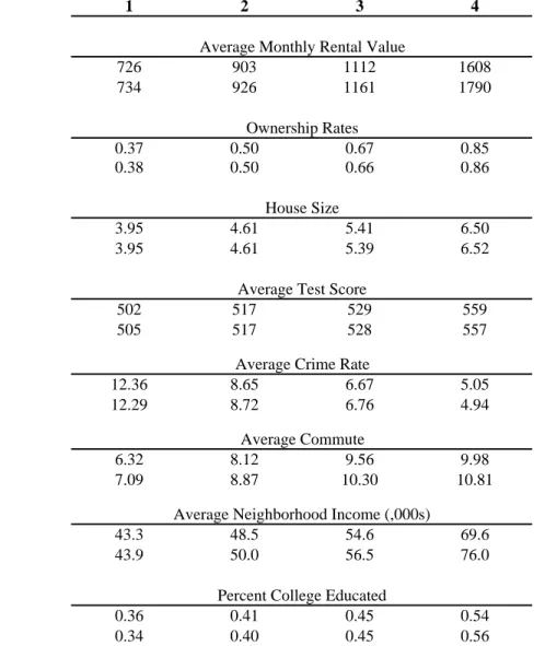
We incorporate school district boundary fixed effects when estimating equation (11). In particular, we create a series of indicator variables for each Census block that equal one if the block is within a given distance of each unique school district boundary in the metropolitan area (e.g., Palo Alto-Menlo Park).25 To show the variation in school quality and neighborhood sociodemographics at school district boundaries, Table 1 displays descriptive statistics for various samples related to the boundaries. The first two columns report means and standard deviations for the full sample while the third column reports means for the sample of houses within 0.25 miles of a school district boundary. Comparing the first column to the third column of the table, it is immediately obvious that the houses near school district boundaries are not fully representative of those in the Bay Area as a whole. To address this problem, we create sample weights for the houses near the boundary.26 Column 7 of Table 1 shows the resulting weighted means, indicating that using these weights makes the sample near the boundary much more representative of the full sample.

25

A number of empirical issues arise in incorporating school district boundary fixed effects into our analysis. A central feature of local governance in California helps to eliminate some of the problems that naturally arise with the use of school district boundaries, as Proposition 13 ensures that the vast majority of school districts within California are subject to a uniform effective property tax rate of one percent. Concerning the width of the boundaries, we experimented with a variety of distances and report the results for 0.25 miles, as these were more precise due to the larger sample size.

26

The following procedure is used: we first regress a dummy variable indicating whether a house is in a boundary region on the vector of housing and neighborhood attributes using a logistic regression. Fitted values from this regression provide an estimate of the likelihood that a house is in the boundary region given its attributes. We use the inverse of this fitted value as a sample weight in subsequent regression analysis conducted on the sample of houses near the boundary.

22

The fourth and fifth columns report means for houses within 0.25 miles of a boundary, comparing houses on the high versus low average test score side of the each boundary; the sixth column reports t-tests for the difference in means. Comparing these differences reveals that houses on the high side cost $53 more per month and are assigned to schools with test scores that are 43-point higher on average.27 Moreover, houses on the high quality side of the boundary are much more likely to be inhabited by white households and households with more education and income. These types of across-boundary differences in sociodemographic composition are what one would expect if households sort on the basis of preferences for school quality. While far less significant, other housing characteristics do vary across the boundaries as well. Consequently, we expect the use of boundary fixed effects to control for much but not all of the variation in unobserved housing and neighborhood quality, thereby giving rise to better estimates of preferences for neighborhood sociodemographics and school quality.28

Characterizing the Housing Market – A Practical Issue. A final practical issue for estimation

concerns the way the choices that characterize the housing market should be defined. This modeling decision essentially corresponds to an assumption regarding the way demand for particular houses in the market is determined. The trade-offs implicit in the required assumption can be seen using a simple example: Consider a city neighborhood with two types of housing structures, one of which is more prevalent than the other, with all houses in the neighborhood selling for the same price. To simplify this discussion, further assume that households have

27

As described in the Data Appendix, we construct a single price vector for all houses, whether rented or owned.

28

In terms of the estimates related to neighborhood sociodemographic characteristics, the key point about using school district boundary fixed effects rather than Census tract fixed effects is that in the boundary case we have a clear sense of what fundamentally leads to the sorting of households across neighborhoods within the region upon which the fixed effect is based. Because we control directly for that cause of the sorting - schooling in this case - we are less concerned that the variation in sorting is related to variation in unobservables within the region upon which the fixed effect is based.

23

identical tastes. In this case, if we characterized the choice set as the two types of structure, we would infer that the more prevalent structure provided higher mean direct utility; this is necessary to explain why more households choose that structure given equal prices. If, on the other hand, we characterized the housing market by randomly drawing a subset of the houses in the neighborhood, we would infer that all of the houses in the neighborhood offered the same utility. We do not see any strong a priori for making one of these choices versus the other. Moreover, given that any definition of ‘type’ would be based only on the limited characteristics observed in the data, we adopt the second option described above, simply characterizing housing types as the 1-in-7 random sample of the houses observed in our Census dataset. This characterization also facilitates comparisons with the hedonic price regression literature; with this characterization of the choice set, a hedonic price regression corresponds to estimating mean preferences under the assumption of no heterogeneity in household tastes.29

Asymptotic Properties of the Estimator. As described in McFadden (1978), an attractive

aspect of the underlying IIA property for each individual is that we can estimate the model using only a sample of the alternatives not selected by the individual. This permits estimation despite having many alternatives – i.e., many distinct house types. More generally, our problem fits within a class of models for which the asymptotic distribution theory has been developed. In this sub-section, we summarize the requirements necessary for the consistency and asymptotic normality of our estimates and provide some intuition for these conditions.

In general, there are three dimensions in which our sample can grow large: H (number of

housing types), N (number of individuals in the sample), or C (number of non-chosen

29

Nothing theoretically prevents estimation of the model under an alternative assumption concerning housing choices. A comparison with corresponding hedonic price regressions is shown in Table 2 and discussed in an

24

alternatives drawn for each individual). For any set of distinct housing alternatives of size H and any random sampling of these alternatives of size C, the consistency and asymptotic normality of the first-stage estimates (δ, θλ) follows directly as long as N grows large. This is the central result of McFadden (1978), justifying the use of a random sample of the full census of alternatives. Intuitively, even if each household is assigned only one randomly drawn alternative in addition to its own choice, the number of times that each house type is sampled (the dimension in which the choice-specific constants are identified) grows as a fixed fraction of N.

If the true vector δ were used in the second stage of the estimation procedure, the consistency and asymptotic normality of the second-stage estimates θδ would follow as long as

HÆ ∞.30 In practice, ensuring the consistency and asymptotic normality of the second-stage estimates is complicated by the fact the vector δ is estimated rather than known. Berry, Linton, and Pakes (2002) develop the asymptotic distribution theory for the second stage estimates θδ for a broad class of models that contains our model as a special case, and consequently we employ their results. In particular, the consistency of the second-stage estimates follows as long as HÆ

∞ and N grows fast enough relative to H such that HlogH Ngoes to zero, while asymptotic

normality at rate H follows as long as H2 N is bounded. Intuitively, these conditions ensure

that the noise in the estimate of δ becomes inconsequential asymptotically and thus that the asymptotic distribution of θδ is dominated by the randomness in ξ as it would be if δ were known.

Given that the consistency and asymptotic normality of the second stage estimates requires the number of individuals in the sample to go to infinity at a faster rate than the number

appendix.

30

25

of distinct housing units, it is important to be clear about the implications of the way that we characterize the housing market in the paper. In particular, we characterize the set of available housing types using the 1-in-7 random sample of the housing units in the metropolitan area observed in our Census dataset. Superficially, this characterization seems to imply that the number of housing types is as great as the number of households in the sample, which appears at odds with the requirements for the establishing the key asymptotic properties of our model.

It is important to note, however, the housing market may be characterized by a much smaller sample of houses, with each ‘true’ house type showing up many times in our large sample. Consider, for example, using a large choice set of 250,000 housing units, when the market could be fully characterized by 25,000 ‘true’ house types, with each ‘true’ house type showing up an average of 10 times in the larger choice set. On the one hand, the 250,000 observations could be used to calculate the market share of each of the 25,000 ‘true’ house types,

with market shares averaging 1/25,000 and the second stage δ regressions based on 25,000 observations. On the other hand, separate market shares equal to 1/250,000 could be attributed to each house observed in the larger sample and the second stage regression based on the larger sample of 250,000. These regressions would return exactly the same estimates, as the former regression is a direct aggregation of the latter. What is important from the point-of-view of the asymptotic properties of the model is not that the number of individuals increases faster than then number of housing choices used in the analysis, but rather that the number of individuals increases fast enough relative to the number of truly distinct housing types in the market. That the number of distinct housing types in the market grows at a rate slower than the number of households seems plausible.

26

5 PARAMETER ESTIMATES

Estimation of the full model proceeds in two stages, as noted, the first stage recovering interaction parameters and vector of mean indirect utilities, the second stage returning the components of mean indirect utility. The first stage of the estimation procedure returns 178 parameters on terms that interact individual and housing/neighborhood characteristics, permitting great flexibility in preferences across different types of households. In particular, the model includes the following household characteristics: household income from non-capital sources, household income from capital sources (a proxy for wealth), race, education, work status, age, the presence of children, and interactions of household income and race. These household characteristics are interacted with many housing and neighborhood attributes including house price, owner-occupancy status,31 number of rooms, the age of the structure, average test score, elevation, population density, crime and eight variables characterizing the neighborhood sociodemographic composition: the fraction of households of each race, the fraction of households college educated, average neighborhood income, and neighborhood income interacted with race. The model also captures the spatial aspect of the housing market by allowing households to have preferences over commuting distance.32

Normalized estimates of the full set of parameters estimated in the first stage of the estimation procedure are reported in Appendix Table 1. To make the discussion of these estimates more transparent, we transform the estimates so that they can be described in terms of

31

We treat ownership status as a fixed feature of a housing unit in the analysis. Thus, whether a household rents or owns is endogenously determined within the model by its house choice. In the model, we allow households to have heterogeneous preferences for home-ownership (a positive interaction between household wealth and ownership, for example, implying that wealthier households are more likely to own their housing unit, as we find below). A single price index is used for owner- and renter-occupied units - see the Data Appendix for details.

32

We treat a household’s primary work location as exogenous, calculating the distance from this location to the location of the neighborhood in question. MWTP estimates for other housing and neighborhood attributes based on a specification without commuting distance are qualitatively similar except for variables that are strongly correlated with employment access such as population density.

27

marginal willingness-to-pay measures (MWTP), reporting these estimates in Tables 2 and 3. The first two columns of Table 2 report measures of the mean MWTP for housing and neighborhood attributes; these estimates are based on a weighted sample of houses33 within 0.25 miles of school district boundaries, with and without including fixed effects, respectively. Comparing the coefficients on the neighborhood sociodemographic characteristics with and without the inclusion of boundary fixed effects (columns 1 and 2) yields the pattern of results one would expect if boundary fixed effects control for fixed aspects of unobserved neighborhood quality that are correlated with neighborhood sociodemographic characteristics in the expected way. In particular, controlling for fixed effects increases the coefficient on percent black (reported at the mean average neighborhood income) from -$285 to -$234; on percent Hispanic from -$37 to $104; and on percent Asian from -$70 to $150. Doing so also reduces the coefficient on the percent of households with a college degree from $186 to $165 and the coefficient on average neighborhood income (/$10,000) from $89 to $85 per month. In this way, the use of boundary fixed effects appears to be effective in controlling for fixed aspects of unobserved neighborhood quality that are correlated with neighborhood sociodemographics, and thus provides an attractive way of estimating preferences for neighborhood sociodemographic characteristics in the presence of this important endogeneity problem.34

Table 3 reports the estimates of the heterogeneity in MWTP for housing and neighborhood characteristics. For ease of comparison, the first column of Table 3 reports the estimated mean MWTP for the changes in housing or neighborhood attributes described in the row headings. The remaining columns report the difference in MWTP associated with the

33

The procedure for constructing sample weights designed to make the boundary sample as representative of the full sample as possible is described in Section 4 above. The estimates reported for the boundary sample without boundary fixed effects are qualitatively similar to those for the full sample.

28

comparison of household characteristics shown in the column heading. So, for example, the first entry of the table implies that, on average, households are willing-to-pay $109 more per month on the margin for an additional room, while the second entry in the first row implies that households with children are willing to pay an average of $31 per month more for a room than households without children.

In almost every instance, the parameter estimates reported in Table 3 seem to have reasonable signs and magnitudes. Focusing specifically on some of the key factors driving the location decision, the results imply that households are willing to pay an average of $50 per month to be an additional mile closer to work or about a dollar per additional mile of actual commuting travel.35 Households with children are willing to pay more for school quality and for an extra room. A number of household characteristics in the model may proxy to some extent for lifetime wealth. Demand for larger homes, owner-occupancy (which may proxy in part for unobserved house quality), and additional rooms in a house is an increasing function of a household’s income from non-capital sources, its income from capital sources, whether a household is working, and a household’s educational attainment.

Turning to the estimated preferences for neighborhood attributes, an interesting distinction arises between tastes for more educated versus higher income neighbors. In particular, the estimates imply a high mean taste for neighbors with more income, but little heterogeneity in taste around this mean. Having controlled for income, however, the estimates reveal preferences for segregation on the basis of educational attainment. In particular, college-educated households are willing to pay a sizeable premium to live with other college-college-educated

34

The analogous hedonic price regressions reported in the remaining columns of Table 2 provides further support for the plausibility of this assertion, as discussed in an Appendix.

29

households, while non-college-educated households would slightly prefer, on average, to live with others who also do not have a college degree.

In examining the estimated heterogeneity in MWTP for neighborhood racial composition, it is important to point out that the parameters corresponding to the interactions between household and neighborhood race in fact combine a number of potential explanations for racial sorting that are indistinguishable in the data. In particular, the estimated interactions combine the effects of (i) discrimination in the housing market (e.g., centralized discrimination against recent immigrants from China), (ii) direct preferences for the race of one’s neighbors (e.g., preferences on the part of a recent immigrant from China to live with other Chinese immigrants), and (iii) preferences for race-specific portions of unobserved neighborhood quality (e.g., preferences for Chinese groceries which are located in neighborhoods with a high fraction of Chinese residents). If one thinks of discrimination as an expression of the racial preferences of the discriminating group concerning the group discriminated against, our model essentially mis-assigns these preferences to the group discriminated against. In this way, the estimated difference in MWTP for black versus white neighbors combines the difference that results from decentralized preferences acted upon in each individual’s own location decision as well as any centralized discrimination that causes black households to appear as if they prefer black versus white neighborhoods more strongly than they actually do. Consequently, the estimates reported in Table 3 are informative about the overall importance of role of racial sorting in the housing market, but, importantly, do not distinguish preferences per se.

The estimated heterogeneity parameters related to race reveal strong segregating racial interactions, with, interpreted literally as preference, households of each race preferring to live

35

Note that the estimate of each individual’s disutility from commuting naturally gives rise to declining rent gradients moving away from employment centers. In this way, the model organically captures any number of

30

near others of the same race. In reading the numbers associated with racial interactions, it is important to keep in mind that these numbers represent the difference in the amount households of the race shown in the column heading would be willing to pay for the corresponding change in neighborhood racial composition compared with white households. So, for example, the $86 per month that characterizes the difference between the MWTP of black versus white households for a 10 percentage point increase in the fraction of black versus white neighbors reflects the sum of what a black household is willing to pay for this increase and what white households would be willing to pay for the opposite change. The parameter estimates also reveal strong segregating preferences for Hispanic and Asian households and that Asian, black, and Hispanic households are more willing to live with minority households of other races than white households are. Finally, the estimates reveal that the strength of these segregating racial interactions does not decline significantly with income. That is, high-income households of each race exhibit a remarkably similar MWTP pattern with respect to the race of their neighbors.

6 GENERAL EQUILIBRIUM SIMULATIONS

We now use the estimated parameters to conduct a general equilibrium simulation designed to examine the impact of an increase in income inequality on the housing market equilibrium. In particular, we calculate the new equilibrium that arises following a 10 percent increase in the income of households in the top income quartile, characterizing the way this change affects a number of aspects of the housing market equilibrium.

The basic structure of solving for a new equilibrium consists of a loop within a loop. The outer loop calculates the sociodemographic composition of each neighborhood, given a set of prices and an initial sociodemographic composition of each neighborhood. The inner loop employment centers within the metropolitan region.