Application of remote sensing and machine learning modeling to post-wildfire debris flow risks

(1)

Michigan Technological University Michigan Technological University

Digital Commons @ Michigan Tech

Dissertations, Master's Theses and Master's Reports 2018

Application of remote sensing and machine learning modeling to

post-wildfire debris flow risks

Priscilla Addison

Michigan Technological University, [email protected]

Recommended Citation

Addison, Priscilla, "Application of remote sensing and machine learning modeling to post-wildfire debris flow risks", Open Access Dissertation, Michigan Technological University, 2018.

https://digitalcommons.mtu.edu/etdr/703

(2)

APPLICATION OF REMOTE SENSING AND MACHINE LEARNING MODELING TO POST-WILDFIRE DEBRIS FLOW RISKS

By

Priscilla E. Addison

A DISSERTATION

Submitted in partial fulfillment of the requirements for the degree of DOCTOR OF PHILOSOPHY

In Geological Engineering

MICHIGAN TECHNOLOGICAL UNIVERSITY 2018

(3)

This dissertation has been approved in partial fulfillment of the requirements for the Degree of DOCTOR OF PHILOSOPHY in Geological Engineering.

Department of Geological and Mining Engineering and Sciences

Dissertation Advisor: Dr. Thomas Oommen

Committee Member: Dr. Ann Maclean

Committee Member: Dr.Qiuying Sha

Committee Member: Dr.Stanley Vitton

(4)

Author Contribution Statement

Chapters 2 and 3 are composed of published material that can be found in peer-reviewed academic journals, and Chapter 4 is work that has been submitted for publication review. Find details of these as follows:

Chapter 2: Addison, P. and Oommen, T., 2018. Utilizing satellite radar remote sensing for burn severity estimation. International Journal of Applied Earth Observation and Geoinformation, 73, pp.292-299

Author Contributions: Addison and Oommen conceptualized the manuscript, and provided revision throughout the study. Addison processed the data and drafted the manuscript.

Permission: Reproduction of this article falls under non-commercial use: “Please note that, as the author of this Elsevier article, you retain the right to include it in a thesis or dissertation, provided it is not published commercially. Permission is not required, but please ensure that you reference the journal as the original source. For more information on this and on your other retained rights, please visit: www.elsevier.com/about/our-business/policies/copyright#Author-rights.”

Article Link: www.sciencedirect.com/science/article/pii/S030324341830432X

Chapter 3: Addison, P., Oommen T., and Sha, Q., 2018. Assessment of Post-Wildfire Debris Flow Occurrence Using Classifier Tree. Geomatics, Natural Hazards and Risk.

Author Contributions: Addison and Oommen conceptualized the manuscript, and provided revision throughout the study. Sha provided statistical modeling expertise, as well as manuscript review. Addison processed the data and drafted the manuscript.

Permission: This is an Accepted Manuscript of an article published by Taylor & Francis Group in Geomatics, Natural Hazards and Risk journal. It has been published as an open access article and hence can be reprinted in a dissertation without requesting further permission. More information can be found here: https://authorservices.taylorandfrancis.com/sharing-your-work/

Chapter 4: Addison, P., and Oommen T., 2018. Post-Fire Debris Flow Modeling Analyses: Case Study of the Post Thomas Fire Event in California. Natural Hazards.

Author Contributions: Addison and Oommen conceptualized the manuscript, and provided revision throughout the study. Addison processed the data and drafted the manuscript.

(7)

Abstract

Historically, post-fire debris flows (DFs) have been mostly more deadly than the fires that preceded them. Fires can transform a location that had no history of DFs to one that is primed for it. Studies have found that the higher the severity of the fire, the higher the probability of DF occurrence. Due to high fatalities associated with these events, several statistical models have been developed for use as emergency decision support tools. These previous models used linear modeling approaches that produced subpar results. Our study therefore investigated the application of nonlinear machine learning modeling as an alternative. Existing models identified the burn severity of wildfires as an important input in their development. Currently, the most widespread approach to obtaining this input is the use of the differenced normalized burn ratio (dNBR) index, which is determined using data from optical sensors on satellites. However, progress of this existing protocol is mostly hampered by the presence of cloud coverage during data acquisition since optical sensors cannot penetrate clouds. Radar sensors on the other hand can penetrate clouds and smoke. This study therefore developed a radar based algorithm to be used as an alternative to the dNBR metric. The results showed the SAR metric to perform even better than the dNBR, with an overall accuracy (OA) of ~60% and Kappa of 0.35 in comparison to an OA of ~35% and a kappa of 0.1 from the dNBR approach. Next we developed a nonlinear machine learning model to predict the likelihood of post-wildfire debris flow occurrences. This produced improved results over the linear

modeling approach with an average sensitivity of 77%, depicting increased ability to predict ~8 out of 10 DF producing basins. Finally, we performed a case study to validate our DF model that showed the model’s robustness in isolating especially high hazard locations. Having these improved models will furnish emergency responders with an increased ability to better assess the associated risks of potential debris flow producing basins and make informed decisions on mitigation and/ or prevention measures.

(8)

1 Introduction

About 350 million ha of land worldwide burn annually as a result of wildfires (van der Werf et al., 2006). This projected coverage is potentially larger in recent years since wildfire frequencies have increased due to the onset of drier climates (Bond-Lamberty et al., 2007; Berman, 2017; Orosco, 2017; Dolan, 2018). Starting from ignition, wildfires leave devastations in their wake, which continue even years after the fire is ended. In fact, history shows most post-fire hazards to be more deadly than the fire itself. An example is the Thomas Fire, in Southern California in December 2017. This fire resulted in two fatalities, whereas a consequent debris flow event in January caused 21 deaths (Berman, 2017; Orosco, 2017; Dolan, 2018).

Post-fire hazards include, but are not limited to emission of greenhouse gases, erosion, flash floods, sediment-laden floods, debris flows, and rock falls (Dixon and Krankina, 1993; Moody and Martin, 2001; Cannon et al., 2009; 2010). Our study focuses on debris flows because historically they are the most fatal of these hazards and their frequencies in western USA are increasing (Cannon and DeGraff, 2009; Eaton, 1935; Bailey et al., 1947; Wells, 1987). A debris flow is a fast-moving, high-density slurry of water, sediments and debris that travels under gravity with enormous destructive power. It usually occurs after periods of intense, short duration precipitation (rainfall, snow melt, etc.) on steep hillsides covered with loose erodible material (Cannon et al., 2010). Debris flows are not exclusive to fire affected areas but a location’s vulnerability

increases significantly after it experiences wildfires (Cannon and Gartner 2005; Canon et al., 2010). The process by which this occurs are outlined as follows. Burning off of the rainfall intercepting vegetation (Kinner and Moody, 2008; Wondzell and King, 2003; Cannon et al., 2010), sealing of the soil pores from the generated ash (Cannon and Gartner, 2005; Larsen et al., 2009), and predominantly, the condensation of organic compounds produce an aftermath of a water repellent soil (DeBano, 2000; Doerr et al., 2000; Cannon and Gartner, 2005; Moody and Ebel, 2012). These processes result in the formation a non-cohesive, water-repellent, bare soil, which is primed for the movement of large volumes of sediment within the burned area and its vicinity.

(9)

Behaviors of debris flows are extremely difficult to predict due to their complex physical structure, trigger mechanisms, and regional variability (Cannon et al., 2010). There are records of studies dating to the 1980s that began the task of detailing the physical

behavior and impact of debris flows (Hungr et al., 1984; Johnson et al., 1991; Cannon et al. 2010; Staley et al, 2017; Prochaska et al. 2008; Santi et al. 2011). Recognition and study of the influence of wildfires on these events began in 1991 when Johnson et al. discovered an increase in volumes of eroded material at locations that had experienced wildfires in their recent past (Johnson et al., 1991). Currently, researchers are focusing on developing statistical models that attempt to predict the probability of post-fire debris flow occurrences. These models are developed by utilizing a number of different descriptive characteristics of a location such as: basin morphology, rainfall

characteristics, burn severity, and soil properties (e.g., Hungr et al. 1984; Bovis and Jakob 1999; Gartner 2005; Gartner et al. 2008; Cannon et al. 2010).

Unsurprisingly, development of these models showed the burn severity of wildfires to be a very important input (Johnson et al., 1991; Cannon et al., 2010; Staley et al., 2017). Generally, a high burn severity basin has a higher likelihood to produce debris flows of larger volumes than one with low severity (Cannon et al., 2010). This makes the burn severity input especially critical to this study. Currently the common approach to

assessing this parameter is by employing satellite remote sensing. In particular, data from optical sensors data have been used extensively to develop algorithms that have proved to be instrumental in mapping burned areas (Koutsias et al., 2000; Justice et al., 2002; Roy et al., 2002; Mitri and Gitas., 2004; Chuvieco et al., 2006; Polychronaki et. al, 2013; Kalogirou et al., 2014; Stroppiana, 2015). The differenced normalized burn ratio (dNBR) is the most common of these algorithms. These optical based approaches, however, have a major disadvantage associated with them, in that their progress can be hampered or even halted by smoke and/or cloud coverage during data acquisition. Substantial smoke and cloud coverage can corrupt an optical image and render it unusable for any analyses to be done. A user who encounters this problem is forced to wait for at least an entire temporal cycle of the satellite of interest for the chance to obtain usable data. For

(10)

emergency situations, this delay can be life threatening and/ or costly. Past research have also shown that the dNBR method of assessing fire severity works well for unburned and highly burned areas but becomes inconsistent in the intermediary severity levels. Some studies found it problematic to clearly delineate intermediate severity burns (Chuvieco et al., 2006; Allen and Sorbel, 2008; Hoy et al., 2008; Murphy et. al., 2008). Radar sensors, on the other hand, can penetrate smoke and clouds and have been used by several

researchers for fire studies (Bourgeau-Chavez, 1997; Rignot et al., 1999; Hoekman et al., 2010; Polyvhronaki, 2013; Kalogirou, 2014), but limited work has been done in the particular area of burn severity determination, especially in the fire prone western United States. With these problem statements in mind, our study set out to complete the

following three objectives:

 Develop a radar-based burn severity estimate to be used as an alternative in emergency situations where there is cloud and/ or smoke coverage.

 Develop a nonlinear machine learning model to predict the likelihood of post-wildfire debris flow occurrences in the western USA.

 Test robustness of developed debris flow model with a case study of recent event occurrence.

We employed machine learning modeling in all three aspects of the study because its algorithms offer flexibility through data driven predictions made by iteratively learning from the input data, as opposed to the strictly static algorithms of some linear models. Machine learning is a type of artificial intelligence that was originally developed to provide computers with the ability to learn without being explicitly programmed (Samuel, 1959). The algorithm was initially developed for the computer science discipline but is now gaining notoriety in other fields due to its robustness. Several models have been developed that use this algorithm to learn from previous computations by searching through data to look for patterns, iteratively re-adjusting until a final robust pattern is found (Samuel, 1959; Fogel et al., 1966; Kohavi and Provost, 1998; Kuhn and Johnson, 2013). Hence, the more data you have to learn from, the better your output. Machine learning modeling can be applied even when the theory behind the data in

(11)

question is not fully understood. Models that use these algorithms have become

widespread in recent years because they have proved to be better at teasing out complex relationships than simple linear models (Kern et al., 2017). Some examples of the success of machine learning modeling include their use in the environmental science field to detect oil spills from satellite imagery (Kubat et al., 1998); geoscience and remote

sensing data (Oommen et al., 2007; 2008; Samui et al., 2012; Gowda et al. 2015); as well as in the medical field to detect cancer tissue samples using microarray expression data (Furey, 2000; Stalin and Kalaimagal, 2016). The surveillance field has used them to develop algorithms for facial recognition (Rowley et al., 1998; Dolecki et al., 2016), whereas the financial world has used them for predicting bankruptcy as well as credit rating (Odom et al., 1990; Wu et al., 2016). There are many other disciplines that have explored machine learning modeling for various complex scenarios that depict the extreme usefulness of this approach and hence, touts its use as an emergency response tool for post-fire debris flow hazards.

To tackle the first aspect of our project, we developed a radar-based metric using the C5.0 decision tree algorithm. This furnished us with an alternative model to use in place of, or in the absence of the optical models. Specifically, we developed a synthetic aperture radar (SAR) based metric aimed at classifying the burn severity into three categories: low severity, moderate severity, and high severity. SAR is a technique that artificially lengthens a radar sensor’s antenna by capitalizing on the flight movement to provide high resolution imagery. The way SAR works is that it transmits microwave energy to a target object, after hitting the target the wave scatters, part of it are lost but others are transmitted back to the SAR receiver. This is measured as the backscatter

value. The amount of waves that are lost depends on the composition and nature of the target object. Its application to burned area studies is that after a surface experiences burn, the loss in vegetative cover causes backscatter variations. These changes are

directly proportional to the degree of burn and therefore make it possible to map the burn severities (Tanase et al., 2015a; Polychronaki et al., 2013). The SAR data that was used was the Japan Aerospace Exploration Agency’s Advanced Land Observing Satellite

(12)

Phased Array type L-band Synthetic Aperture Radar (ALOS PALSAR) obtained from the Alaska Satellite Facility. Details of this study have been provided in the Chapter 2 of this dissertation.

Moving on to the issue of debris flows prediction, we again employed the machine learning-based decision tree algorithm to develop a nonlinear model that predicts the probability of debris flow generation after wildfires. Previous studies, mostly by

researchers at the United States Geological Survey (USGS), had predominantly employed linear models, specifically the logistic regression model (Cannon and Gartner 2005, Cannon et al., 2010, Staley et al., 2017). The logistic regression approach is advantageous because it considers simple linear classification boundaries, making model development simple as well as easy to interpret. However, its simplicity is a detriment to it in debris flow modeling due to its complex triggering and flow mechanics. Up until 2017, the best model reported a sensitivity of 44% (Cannon et al., 2010) — this translates to an

approximate 4 out of 10 debris flow producing basins being correctly isolated. This was not ideal and hence, Staley et al., 2017 used a more data rich sample to develop an

updated logistic regression model with an improved sensitivity of 83%. It, however, had a specificity of 58%, which means that ~6 out of 10 “debris flow safe” locations will be correctly predicted. Although this updated model provides an increased ability to isolate more vulnerable areas, it held the risk of desensitizing the public, due to the likelihood of producing high false positive predictions. We therefore proposed the use of the C5.0 decision tree algorithm to investigate if higher predictive capabilities could be harnessed from this nonlinear machine learning approach. Details of this have been provided in Chapter 3 of this dissertation.

Finally, the fourth chapter of this dissertation sought to validate the developed debris flow prediction model by considering a case study. We applied both the C5.0 tree and USGS’ logistic regression models to a recent fire that happened in Southern California, the Thomas Fire. This fire, which was the largest in California’s recent past at time of its ignition, occurred from December 4, 2017 to January 12, 2018 and consumed ~114,000 ha of land. Before the fire could be fully contained a major storm occurred on January 9,

(13)

2018, which triggered debris flows within the burned area, inundating several

communities downstream in the Santa Barbara and Ventura Counties. Using this location as a case study, we validated our C5.0 tree model as well as compare its predictive

strength with that of the logistic regression model. Details of this have also been provided in Chapter 4 of this dissertation.

(14)

2 Utilizing Satellite Radar Remote Sensing for Burn

Severity Estimation

1

Abstract: The increasing knowledge in the capabilities of satellite imagery to hazard applications is especially useful in emergency situations where timing and ability to cover large areas is of the essence. For optical imagery, cloud coverage can corrupt an image rendering it unusable for intended emergency analyses. This study proposes the use of Synthetic Aperture Radar (SAR) imagery for burn severity analysis for western United States sites, as an alternative to its optical based counterpart, differenced normalized burn ratio (dNBR). Unlike optical sensors, the radar sensor is an active sensor that is able to penetrate clouds and smoke, an attribute that is crucial in emergency situations where immediate burn severity data are needed to assess the vulnerability of fire affected areas to post-fire hazards. Using C5 decision tree algorithm we developed a SAR-based metric that attempts to classify burn severities of fire affected locations in the western USA. We then compared the performance of this developed metric to that obtained by the existing dNBR metric, to determine if there is any merit to its adoption as an alternative for the western USA landscape. The results showed the SAR approach to produce higher validation metrics in comparison to the dNBR. It had an overall accuracy and kappa of 60% and 0.35, respectively, in comparison to the 35% and 0.1 of the dNBR approach. This shows an improved ability to quickly obtain burn severity data and make better informed decision in emergency situations.

1_{This material has been published as an Open Access article in the}_{International Journal of Applied Earth}

(15)

2.1 Introduction

The hazards associated with a wildfire continue even after it is contained. A wildfire’s aftermath usually results in the loss of vegetative cover, leaving the ground exposed and vulnerable to a plethora of post-fire hazards. These hazards include erosion, sediment flows, rock falls, flash floods, debris flows, and release of greenhouse gases into the atmosphere (Dixon and Krankina, 1993; Moody and Martin, 2001; Cannon et al., 2009; 2010). The intensity of such post-fire hazards are usually exacerbated by the severity of the fire. Emergency response teams therefore need immediate access to burn severity maps to enable them to assess the vulnerability of fire affected areas to post-fire hazards (Cannon et al., 2010; Staley et al., 2016; Kern et al, 2017). The United States Department of Agriculture (USDA), for example, has formed a dedicated team— Burned Area

Emergency Response (BAER)— whose mission is to rapidly evaluate severity of fires and their implications on Federal lands and prescribe emergency stabilization treatments. The BAER team works on a short turnaround time because their activities have to be completed before the next major storm. Their work therefore begins even while the wildfire is still ongoing because it is imperative that stabilization measures (reseeding with quick-growing species, mulching, building slope breakers, etc.) are applied as soon as possible (Witt, 1999)

Currently, the common approach to determining burn severity of an extensive area is by employing satellite imagery since they provide objective estimates and cover wider investigative areas (Key and Benson, 2006; Miller and Thode, 2007; Parks et al., 2014). In particular, optical satellite data have been used extensively and proven to be useful for mapping burned areas (Koutsias et al., 2000; Justice et al., 2002; Roy et al., 2002; Mitri and Gitas., 2004; Chuvieco et al., 2006; Stroppiana, 2015). The optical approach,

however, has a major disadvantage of being hindered by cloud coverage and smoke from ongoing wildfires (Schroeder et al., 2008; Wooster et al., 2013; Allison et al., 2016). Substantial cloud coverage and/or smoke can mask an optical image and render it

unusable for the intended burn severity analysis. A user who encounters this misfortune is forced to wait for at least an entire temporal cycle of the satellite—16 days, in the case of

(16)

Landsat—for the chance to obtain usable data. For potential emergency hazards, this delay can be life threatening and/or costly. Also, studies have shown that the most widely used optical approach, the differenced normalized burn ratio (dNBR), shows

inconsistencies in the intermediary burn severity levels. Some studies found it

problematic to clearly delineate intermediate severity burns (Chuvieco et al., 2006; Allen and Sorbel, 2008; Hoy et al., 2008; Murphy et. al., 2008). Finally, the dNBR index is an absolute measure of landscape (vegetation) change, hence it fails to take into account the heterogeneous nature of landscapes. That is, for the same intensity of burn, a pixel with sparse pre-fire vegetation will measure a small change (lower dNBR) even if it

experienced a high severity burn; whereas its counterpart with dense pre-fire vegetation will register a high change (higher dNBR).This becomes problematic when a user

encounters a landscape with different vegetation types and densities and try to rank them on the same burn severity scale (Miller and Thode, 2007; Parks et al., 2014).

We are therefore proposing an alternate approach in this study: radar burn severity estimation. Unlike optical sensors, the radar sensor is an active sensor that is able to penetrate clouds and smoke, an attribute that is crucial in emergency situations. Radar satellite sensors use a technique known as synthetic aperture radar (SAR), which is basically the artificial lengthening of a sensor’s antenna by capitalizing on the flight movement to provide high resolution imagery. SAR uses microwave energy to quantify and discern between ecological processes by measuring the differences in scattering based on the roughness of the target surface. Variation in the dielectric constant of target objects plays a central role in determining the intensity (backscatter) of the microwave energy that is received and processed into the resulting SAR image (Kasischke et al., 1997). Its application to burned area studies is that after a surface experiences burn, the loss in vegetative cover causes scattering variations. These changes are directly

proportional to the degree of burn and therefore make it possible to map the burn

severities (Tanase et al., 2015a; Polychronaki et al., 2013). The use of SAR to determine burn severity is in no way novel, however, it is a fairly new application area with limited literature currently available (Tanase et al., 2010a, 2010b, 2015a, 2015b). Further, the

(17)

existing studies focus predominantly on Mediterranean forests. The signature of SAR’s measurement is unique to different vegetation types, hence with the landscape of the western USA being different from the Mediterranean landscape, an extensive study like this one with unique concentration on the western USA is warranted. Finally, noting the difficulty of the dNBR approach to account for the heterogeneous nature of landscapes we will consider relative measures of SAR burn severity by averaging over the pre-burn condition of each landscape to account for its relative change.

2.2 Methods

2.2.1 Study Area

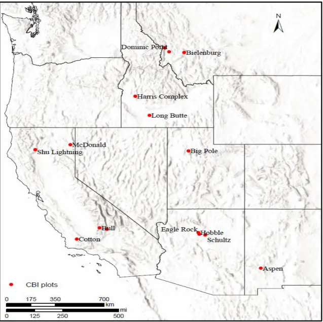
Our study considered 15 fires that occurred across six States in the fire-prone western USA (Figure 2.1, Table 2.1) from 2008 to 2010. These fires were chosen out of the 37 fires in the FIRESEV (FIRE SEVerity mapping system project) database (Dillon et al, 2011a; Sikkink et al., 2013) because they were the ones with documented containment dates. FIRESEV was a project funded by a Joint Fire Sciences Program “geared toward providing fire managers across the western United States with critical information for dealing with and planning for the ecological effects of wildfire at multiple levels of thematic, spatial, and temporal detail” (Dillon et al, 2009). This project collected ground-based burn severity data on 37 fires that occurred in the western USA from 2008-2010 (Sikkink et al., 2013).

2.2.2 Field Data

The field protocol used in the FIRESEV project was the Composite Burn Index (CBI), which assesses the burn severity of a landscape on a continuous scale by visually

examining vegetation conditions of 90-meter diameter plots in the aftermath of a fire with respect to the condition of vegetation before the fire. Values range from 0 (unburned) to 3 (high severity) for any given plot (Key and Benson, 2006).

(18)

Figure 2.1 Study area of western USA showing the 15 fires from 2008-2010 from the FIRESEV database.

Setting CBI thresholds is arguably as much an art as science, so depending on study location and study focus, threshold values could differ for different studies. After doing some preliminary explorations of different thresholds, we decided on the ranges proposed by Key and Benson, 2005 (Table 2.2). The only exception was the unburned class that was set at a threshold of 0.1 because preliminary analysis showed the noted range limit of 0.5 encapsulated most of the low severity samples. Documentation on the FIRESEV project noted that it was predominantly geared towards isolating high severity burn

(19)

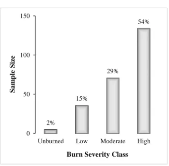
locations (Dillon et al, 2011b) therefore there was an intentional sample bias towards this class, which was evident even in the subset of data we obtained (Figure 2.2); this further gave confidence to the class thresholds set. The unburned class comprised ~2% of the sample size, so we removed them from further analyses to prevent this extreme class imbalance.

Table 2.1. List of fires used in the study

Fire Name State Ignition Date

Containment Date

Eagle Rock Arizona 6/11/10 6/28/10

Hobble Arizona 8/30/10 10/15/10 Schultz Arizona 6/20/10 7/7/10 Bull California 7/26/10 8/10/10 Cotton California 5/15/10 5/17/10 Indian California 7/18/10 7/24/10 McDonald California 7/27/10 8/10/10

Shu Lightning California 6/21/08 7/20/08

Harris Complex Idaho 8/27/10 9/4/10

Long Butte Idaho 8/21/10 8/31/10

Bielenburg Montana 7/12/09 10/1/09

Dominic Point Montana 7/25/10 8/7/10

Kootenai Creek Montana 7/12/09 8/5/09

Aspen New Mexico 6/6/10 6/26/10

(20)

Table 2.2 CBI and dNBR severity category definitions. Bilinear interpolation was used to cross-reference CBI values with dNBR values

Class CBI dNBR Description

Unburned 0.00 – 0.10 0.00 – 0.10

Location experienced no fire. This may also include a location that recovers quickly after fires. Low 0.10 – 1.24 0.10 – 0.27 Minimal vegetation consumption;

patches of scorched foliage.

Moderate 1.25 – 2.24 0.27 – 0.66

The landscape exhibits transitional conditions between low and high severity characteristics described.

High 2.25 – 3.00 > 0.66

~ 90% to total consumption of vegetation. Sites normally exhibit over 50% cover of newly exposed mineral soil or rock fragments

Figure 2.2 Percentage of the different CBI burn severity classes from the FIRESEV database 2% 15% 29% 54% 0 50 100 150

Unburned Low Moderate High

Sa

m

ple

Size

(21)

2.2.3 Remote Sensing Data

2.2.3.1 Optical Burn Severity Determination

The dNBR index determines burn severities by harnessing the spectral values of the near infrared (NIR) and short wave infrared (SWIR) wavelengths. NIR records high

reflectance values for healthy vegetation and low values for burned vegetation; whereas the converse is true for SWIR; low reflectance in healthy vegetation and high reflectance in burned areas. With these intrinsic signatures, the normalized burn ratio (NBR)

(equation 1) was developed to map burn areas. A high NBR value generally indicates healthy vegetation whereas a low value indicates low or no vegetation, such as a result of fire. To go a step further to quantify different severity classes, the dNBR (equation 2) was developed as a temporal change detection metric. This metric runs from -2 to +2, with high positive values corresponding to severely burned locations.

𝑁𝐵𝑅 =𝑁𝐼𝑅 𝑏𝑎𝑛𝑑−𝑆𝑊𝐼𝑅 𝑏𝑎𝑛𝑑

𝑁𝐼𝑅 𝑏𝑎𝑛𝑑+𝑆𝑊𝐼𝑅 𝑏𝑎𝑛𝑑 (1)

𝑑𝑁𝐵𝑅 = 𝑁𝐵𝑅_{𝑝𝑟𝑒𝑓𝑖𝑟𝑒}− 𝑁𝐵𝑅_{𝑝𝑜𝑠𝑡𝑓𝑖𝑟𝑒} (2)

Cloud-free pre- and post- images were downloaded from Landsat 5 Thematic Mapper (TM). These images were downloaded as Level 1 products (geometrically and

radiometrically corrected) from USGS’ Earth Explorer website. Burn severity for each scene was determined using equations (1) and (2) with bands 4 and 7 corresponding to the NIR and SWIR infrared wavelengths, respectively. We then extracted the dNBR values to correspond to each CBI plot location using bilinear interpolation, as a past study showed this approach to give representative values corresponding to the CBI plots (Parks et al., 2014). Bilinear interpolation is a resampling approach that uses the four closest pixels of an input raster, with a user defined statistic metric, to determine the value of the output raster. The statistic metric used for our study was the mean, which was adjusted to account for the distance of each of the four closest rasters to the centroid of the output cell. This resampling step was necessary to account for the extent of the CBI plot, which is unlikely to fall within a single raster pixel. The continuous dNBR values were then

(22)

classified into their respective severity classes of low, moderate, and high (Table 2.2). This four class categorization is known in the fire community as BARC-4 (burned area reflectance classification, using 4 classes).

2.2.3.2 Radar Burn Severity Determination

SAR scattering is sensitive to vegetation structure and biomass. Removal of leaves and branches from trees after wildfires alters the scattering mechanisms causing temporal variations of the backscatter coefficient (Polychronaki et al., 2013). This temporal alteration makes it possible to map burn severity. The wavelength and polarization of the SAR sensor strongly influence the accuracy of the output. The higher the wavelength the more penetration the SAR signals are able to achieve. The higher wavelength of the L-band (24 cm) therefore allows it to penetrate vegetation canopy and interact with large branches, stems, and the forest floor (Le Toan et al. 1992), which makes it possible to discern burned structures from unburned ones. Conversely, the X- and C- bands, by virtue of their lower wavelengths (5.6 cm and 3 cm, respectively), have lower penetration capabilities; scattering occurs only in the upper few centimeters of the forest canopy making them less favorable in burn severity applications (Tanase et al., 2010a, 2010b, 2015a, 2015b). In terms of polarizations, the cross-polarized state (HV) has been shown to be sensitive to volume changes hence, the removal of leaves and branches by fire and consequent thinner, dryer vegetation results in a decreased backscatter. These processes translate to the needed contrast in SAR image to discern changes.

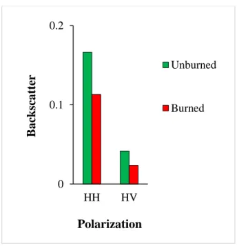
The Advanced Land Observing Satellite Phased Array type L-band Synthetic Aperture Radar (ALOS PALSAR) was the sensor employed in our studies. This was because it is the only L-band sensor that was in operation during our investigative period and also that its data are readily available at no cost. Pre- and post- fire data were downloaded through the Alaska Satellite Facility (ASF) as fine beam dual polarization (FBD) products, which meant that they had both HH and HV polarization information. A preliminary assessment of the mean backscatter values for the study locations pre- and post- fire conditions showed that unburned locations recorded higher backscatter coefficients in comparison to

(23)

their burned counterparts for both HH and HV polarizations (Figure 2.3). This supports the theory found in earlier literature.

The ALOS PALSAR data were also downloaded as radiometrically terrain-corrected (RTC) products from ASF. This meant that single look complex (SLC) data had already been converted to radiometrically and terrain geo-coded data by ASF. By this, co-registering was done for scenes obtained from the same sensor and track. Multi-looking had also been performed to obtain representative pixel sizes as well as reduce the

characteristic speckle noise associated with SAR data. For images with fully developed speckle noise, further filtering had been done by applying a sensor-suitable adaptive or non-adaptive filter; keeping in mind to preserve good radiometric as well as spatial resolution (Bernhard et al., 2011; Gimeno et al., 2004). Geocoding had finally been carried out using the best available digital elevation model (DEM). Two sets of data were downloaded for each fire for pre- and post- fire scenarios, respectively.

Figure 2.3 A plot of mean backscatter values for the fifteen burned areas considered in this study for before (green) and after (red) the fires.

0 0.1 0.2 HH HV B ac k sc att er Polarization Unburned Burned

(24)

Next, we developed the following absolute and relative predictors from the HH and HV backscatter data to quantify the landscape changes due to wildfire:

𝐴𝑏𝑠_𝐻𝐻 = 𝐻𝐻_𝑝𝑟𝑒− 𝐻𝐻_{𝑝𝑜𝑠𝑡} (3) 𝐴𝑏𝑠_𝐻𝑉 = 𝐻𝑉𝑝𝑟𝑒− 𝐻𝑉𝑝𝑜𝑠𝑡 (4) 𝑅𝑒𝑙_𝐻𝐻_1 =𝐻𝐻𝑝𝑟𝑒−𝐻𝐻𝑝𝑜𝑠𝑡 𝐻𝐻𝑝𝑟𝑒 (5) 𝑅𝑒𝑙_𝐻𝑉_1 =𝐻𝑉𝑝𝑟𝑒−𝐻𝑉𝑝𝑜𝑠𝑡 𝐻𝑉𝑝𝑟𝑒 (6) 𝑅𝑒𝑙_𝐻𝐻_2 =𝐻𝐻𝑝𝑟𝑒−𝐻𝐻𝑝𝑜𝑠𝑡 √𝐻𝐻𝑝𝑟𝑒 (7) 𝑅𝑒𝑙_𝐻𝑉_2 =𝐻𝑉𝑝𝑟𝑒−𝐻𝑉𝑝𝑜𝑠𝑡 √𝐻𝑉𝑝𝑟𝑒 (8)

Equations (3) and (4) to give the absolute changes of the landscape after fires, whereas equations (5) to (8) give the relative changes with respect to the existing condition on the ground before the fire. We extracted each of these predictors to correspond to the CBI plots using bilinear interpolation, as was done for the dNBR data. Land Cover Data We observed the existence of different vegetation types across the six States that were investigated. Past studies indicate that the differences in the moisture content and

individual components of different vegetation types results in unique dielectric constants (Rignot et al, 1994; Kasischke et al., 1997; Wegmuller and Werner, 1997). The different dielectric constants cause different vegetation groups to have different scattering and attenuating responses to the microwave energy transmitted by radars (Kasischke et al., 1997). Therefore, we obtained land cover data from the National Land Cover Database (NLCD) from the United States Department of Agriculture’s geospatial data gateway to quantify the broad land cover types. Preliminary analyses showed improved results when land cover data was integrated into model development. Our sites comprised the

(25)

These were coded as three separate dummy variables to be used as predictors and were extracted for each CBI plot using nearest neighbor resampling method. With these three dummy variables, together with the six predictors from equations (3) – (8), we had a total of nine candidate predictors for developing our model.

2.2.4 Data Analyses

2.2.4.1 C5.0 Algorithm

The algorithm used for this study was the C5.0 decision tree (Quinlan, 1993). It is a simple method that uses inductive inference to approximate discrete-valued functions. It is robust to noisy data and capable of learning mutually exclusive expressions. Its algorithm works by sorting the data from a base decision into smaller, more

homogeneous groups. It does this by developing a general decision called the root, then branching out from there with other more specific decisions known as branches, till it gets to a decision that produces homogeneous samples, which are then assigned a

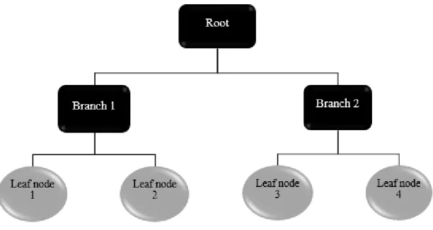
classification known as the leaf (Kuhn and Johnson, 2013). This represents a typical tree structure, hence, the name decision tree. Figure 2.4 gives a schematic of a simplified tree with one root, two branches and four leaves.

At each node, each predictor is tested to assess how well it alone separates the training data according to the target classification. The process is repeated on each new subset until a subset contains only samples of a single class, or the partitioning tree has reached a predetermined maximum depth. Trees are grown to their maximum size and then a pruning step is usually applied by removing a decision’s precondition if the accuracy of the decision improves without it. This is done to avoid overfitting to the training data. The C5.0 tree algorithm uses boosting in its model training process, which works by combining average model decisions together to improve overall model performance of the final output.

(26)

Figure 2.4 Schematic of a simplified decision tree with a root, two branches and four leaf nodes

2.2.4.2 Model Development

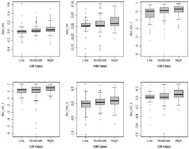
Figure 2.5 shows boxplots of the six continuous predictors (excluding the three land cover predictors) as they relate to the different burn severity classes from the CBI data. A look at this shows the low and moderate severity classes to have mostly similar median values. This likely due to the fact that there were not as many samples for these two as there were for the high severity class. Preliminary data pre-processing steps taken to ensure optimal model performances included omitting observations with missing values and testing for predictor degeneracy.

(27)

Figure 2.5 Boxplots showing how the six continuous predictor variables vary with the CBI classes of low, moderate, and high burn severity.

We then run a predictor selection routine that tested the performance of candidate models with successively fewer predictors (Dillon et al., 2011b and Birch et al., 2015). By this, we assessed the influence of each individual predictor on the model as a whole. We examined the variable importance from the C5.0 tree modeling process. With each model run, C5.0 tree calculates variable importance by randomly permuting the values of each variable, one at a time, and calculating the change in overall model performance (mean decrease in accuracy) as a result. We determined the rankings of stable predictor importance by running 10 reproducible C5.0 tree models with all the nine predictors. From here, we determined a single value of importance for each predictor from the mean variable importance of all 10 candidate models and ranked them (1= highest importance;

(28)

9 = least importance). The results identified REL_HV_1, evergreen forest, and Abs_HV to be most informative, having an aggregated ranking of less than a threshold of 50 (Figure 2.6).

Using the three final predictors, REL_HV_1, evergreen forest, and Abs_HV, an 80-20 data sampling split was made without replacement. 80% of the data was used to train the model and 20% was used to validate it. This split was done using stratified random sampling to ensure that representative distributions of the response variable were sampled in each set since our class sizes were imbalanced. A leave-one-out cross validation

resampling was applied to determine the number of trials needed to achieve optimal model performance. An interval of 1 – 30 was set as the candidate for this process. The results from the resampling were then aggregated into a performance profile which revealed optimal number of trials to be 6. Setting this as the optimum number of trials, the model was developed a final time using the entire training data.

Figure 2.6 Aggregated ranking of variable importance for 10 candidate model runs for all nine predictors 9th 7th 8th 6th 5th 4th 3rd 2nd 1st 0 20 40 60 80 100 Herbaceous Shrub Rel_HH_2 Rel_HH_1 Rel_HV_2 Abs_HV Abs_HH Evergreen_forest Rel_HV_1 Aggregated rank Predi ct or

(29)

2.2.4.3 Model Validation

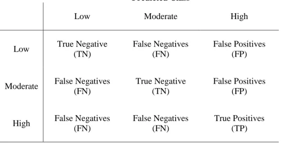
To first establish the baseline to compare our SAR analyses to, we determined a confusion matrix (Table 2.3) using the CBI values for the 15 fires as the reference data and the BARC-4 data as the predictor. We then tested our developed SAR model on the initial 20% validation set that was retained after preprocessing.

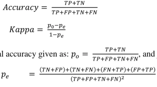
From this we determined the overall accuracy (Eq. 9), which measures the overall performance of the model in correctly identifying the three different burn severity classes. It ranges from 0 to 1, with 0 representing a model with no predictive capability and 1 representing a perfect model. Cohen’s Kappa (Eq. 10), also provides a measure of the overall performance of the model by measuring the precision between predictions and observations while correcting for chance agreements (Cohen, 1960). This statistic takes into account the possibility of chance predictions hence it tends to be more conservative. Typical values from 0.30 – 0.50 on a scale of -1 to 1 represent a model with reasonable agreement (Kuhn and Johnson, 2013).

Table 2.3 A three class confusion matrix, setting the “high” class as the true positive

Predicted Class

Low Moderate High

Ac

tual

Class

Low True Negative

(TN)

False Negatives (FN)

False Positives (FP)

Moderate False Negatives (FN)

True Negative (TN)

False Positives (FP)

High False Negatives (FN)

False Negatives (FN)

True Positives (TP)

(30)

𝐴𝑐𝑐𝑢𝑟𝑎𝑐𝑦 = 𝑇𝑃+𝑇𝑁

𝑇𝑃+𝐹𝑃+𝑇𝑁+𝐹𝑁 (9)

𝐾𝑎𝑝𝑝𝑎 = 𝑝0−𝑝𝑒

1−𝑝𝑒 (10)

where po is the total accuracy given as: 𝑝𝑜 =

𝑇𝑃+𝑇𝑁

𝑇𝑃+𝐹𝑃+𝑇𝑁+𝐹𝑁, and pe is the random

accuracy given as: 𝑝_𝑒 = (𝑇𝑁+𝐹𝑃)+(𝑇𝑁+𝐹𝑁)+(𝐹𝑁+𝑇𝑃)+(𝐹𝑃+𝑇𝑃)

(𝑇𝑃+𝐹𝑃+𝑇𝑁+𝐹𝑁)2

2.3 Results and Discussion

Values of the continuous dNBR index ranged from -0.20 to 0.84; these corresponded to continuous CBI values from 0 to 3 across the 15 burned areas. A plot of the continuous values of the CBI confirmed the challenges of the dNBR having difficulty in

differentiating between moderate and high severity burns, as there did not seem to be much separation between these two classes (Figure 2.7).

Figure 2.7 A plot of continuous values of the CBI against the continuous values of dNBR 0 1 2 3 -0.2 0 0.2 0.4 0.6 0.8 1 CBI dNBR

(31)

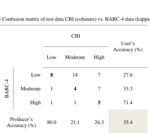
A baseline confusion matrix between CBI and the BARC-4 data also confirmed this difficulty, as only ~21% and ~26% of the moderate and high severity classes,

respectively, were correctly identified (Table 2.4). The confusion matrix shows the low severity class to have the highest producer’s accuracy of 80%, which goes to show that the reflectance-based BARC-4 does a good job of correctly predicting low severity locations, however, its ~28% user’s accuracy is problematic because here, a large count of moderate and high severity locations are being incorrectly classified as low severity. With this baseline established, we developed our SAR model with the three final

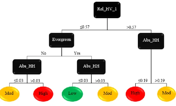
predictors to check against. Figure 2.8 and Table 2.5 show the breakdown of the tree that was developed from our C5.0 tree algorithm. This tree had one root node, four branches and six leaves. The algorithm identified the Rel_HV_1 predictor as its root. This makes the Rel_HV_1 predictor the most important, as it forms the base of every decision made. It therefore means that relating the response of the landscape to its condition before the fire occurrence makes it possible to better discern the different severity classes.

Table 2.4 Confusion matrix of test data CBI (columns) vs. BARC-4 data (kappa = 0.10)

CBI

User’s Accuracy (%) Low Moderate High

B ARC -4 Low 8 14 7 27.6 Moderate 1 4 7 33.3 High 1 1 5 71.4 Producer’s Accuracy (%) 80.0 21.1 26.3 35.4

(32)

Figure 2.8 Break down of the decisions for developing the final SAR burn severity model

The Evergreen decision branch generally classified locations where this land cover was present as low to moderate severity and locations without evergreen forests as moderate to high severity. This means that the likelihood of having a high severity burn is low when evergreen forests are present. A critical look at this predictor confirmed that the low severity locations had the majority of this land cover type whereas the high severity had the least (Figure 2.9).

≤0.57 >0.57

No

≤0.03 >0.03 ≤0.03 >0.03 ≤0.19 >0.19 Yes

(33)

Table 2.5 Summary of decision paths for each leaf node

Leaf Decisions Burn Severity

1 Rel_HV1 ≤ 0.57 Evergreen = No Abs_HH ≤ 0.03 Moderate 2 Rel_HV1 ≤ 0.57 Evergreen = No Abs_HH > 0.03 High 3 Rel_HV1 ≤ 0.57 Evergreen = Yes Abs_HH ≤ 0.03 Low 4 Rel_HV1 ≤ 0.57 Evergreen = Yes Abs_HH > 0.03 Moderate 5 Rel_HV1 > 0.57 Abs_HH ≤ 0.19 High 6 Rel_HV1 ≤ 0.57 Abs_HH > 0.19 Moderate

(34)

Figure 2.9 Plot showing percent coverage of evergreen vegetation in the different burn severity classes.

The HH polarization also played an integral role in the developed model, as it was the final determinant in all the six decisions. This was unexpected because past studies showed the cross-polarized HV to be a much better discerner of burn severity classes than the co-polarized HH polarization. The argument was that the strength of the backscatter from the HV polarization was much higher since by virtue of the transmitted waves going in horizontally and received vertically translates to volumetric scattering. However, we see here that the HH polarization, though not as important as the HV polarization, is crucial in discerning between burn classes.

Some other observations were that generally a low Abs_HH corresponded to low severity classification whereas higher Abs_HH values corresponded to the higher severity classes. This is intuitive because from equation 3, low Abs_HH is obtained when pre- and post- backscatter values are close to each other in magnitude. This is what is to be expected in

0 10 20 30 40 50

Low Moderate High

E ve rgr ee n F or est Cove rage (% ) Burn Severity

(35)

a low severity burn because the landscape would not have experienced that much change to translate to a large difference in recorded values. The converse is also true, as higher Abs_HH corresponded to higher severity burns.

Testing the 20% validation data set that was retained during model development on our final model gave the results presented in Table 2.6. An overall accuracy of ~60% and a kappa of 0.35 for a three-class model show good predictive performance. The model performed better in identifying moderate and high severity locations but had difficulty with the low severity locations. The fact that the low severity had the least sample size (15%) likely contributed to this underperformance, hence we are hopeful that

improvement will be possible with a data rich model. Comparing this to the results obtained from the dNBR approach (Table 2.5) clearly shows the SAR approach to perform much better.

Table 2.6 Confusion matrix of test data CBI vs. SAR classified data (kappa = 0.35)

CBI

User’s Accuracy (%)

Low Moderate High

S AR Low 1 1 0 50.0 Moderate 7 15 6 53.6 High 2 3 13 72.2 Producer’s Accuracy (%) 10.0 78.9 68.4 60.4

(36)

Finally to test the importance of the land cover input, the model was tested without the Evergreen predictor. This resulted in an accuracy of 48% and kappa of 0.14. This is a clearly mediocre model in comparison and proves that knowledge of the land cover type is necessary for radar burn severity estimation. It is even possible that dNBR approach might be improved with a land cover input as well and future studies can look into it.

2.4 Conclusions and Future Work

The main focus of this study has been to develop a SAR based metric aimed at classifying the burn severity of locations in the western USA that have experienced wildfires as an alternative to the commonly used dNBR metric. We consequently compared the performance of SAR approach to the accepted dNBR approach to determine if there is any merit to its adoption as an alternative in the western USA landscape. The results showed the SAR approach to produce higher validation metrics in comparison to the dNBR. It had an overall accuracy and kappa of ~60% and 0.35

respectively in comparison to the ~35% and 0.1 of the BARC-4 data.

Generally, smaller differences in backscatter values for pre- and post- fire data translated to lower burn severities and vice versa. This was intuitive because for low severity, the landscape would not have experienced much change, thereby translating to lower differences in scattering of the radar signals and consequently, lower differences in backscatter values. Another noteworthy discovery was that the presence of evergreen forests seemed to limit the severity of fires.

Overall, this developed SAR based metric showed improved results and can therefore be recommended as an alternative to the optical sensor approach of the dNBR. Also,

because the radar signals of SAR can penetrate clouds, this will be even more beneficial in emergency situations where burn severity information is needed right away to

implement stabilization measures on unstable slopes.

FUNDING: This research did not receive any specific grant from funding agencies in the public, commercial, or not-for-profit sectors.

(37)

3 Assessment of Post-Wildfire Debris Flow Occurrence

Using Classifier Tree

2

Abstract: Besides the dangers of an actively burning wildfire, a plethora of other hazardous consequences can occur afterwards. Debris flows are among the most hazardous of these, being known to cause fatalities and extensive damage to

infrastructure. Although debris flows are not exclusive to fire affected areas, a wildfire can increase a location’s susceptibility by stripping its protective covers like vegetation and introducing destabilizing factors such as ash filling soil pores to increase runoff potential. Due to the associated dangers, researchers are developing statistical models to isolate susceptible locations. Existing models predominantly employ the logistic

regression algorithm, however, previous studies have shown that the relationship between the predictors and response is likely better predicted using nonlinear modeling. We therefore propose the use of nonlinear C5.0 decision tree algorithm, a simple yet robust algorithm that uses inductive inference for categorical data modeling. It employs a tree-like decision making system that makes conditional statements to split data into

homogeneous classes. Our results showed the C5.0 approach to produce stable and higher validation metrics in comparison to the logistic regression. A sensitivity of 81% and specificity of 78% depicts improved predictive capability and gives credence to the hypothesis that data relationships are likely nonlinear.

2_{This material has been published as an Open Access article in the Geomatics, Natural Hazards and Risk}

(38)

3.1 Introduction

An average of 350 million hectares of land are affected annually by wildfires worldwide (van der Werf et al., 2006). There are predictions of even further increase in these occurrences with increasing trends in temperature (Westerling et al., 2006;

Bond-Lamberty et al., 2007; Miller et al., 2009; Flannigan et al., 2009). The hazards associated with a wildfire continues even after it is contained. Its aftermath can yield itself to a spectrum of post-effects, of which debris flows are at the most disastrous end (Brock et al., 2007; Cannon et al., 2010). Debris flows are fast-moving, high-density slurry of water, sediments and debris that travels under gravity and are endued with enormous destructive power (Cannon and Gartner 2005, Cannon et al., 2010, Staley et al., 2017). They usually occur after periods of intense, short duration precipitation on steep hillslopes covered with loose erodible material (Cannon et al., 2010). They are very destructive to anything in their paths and are usually associated with fatalities. A recent event occurring on January 09, 2018 in Montecito, California resulted in 21 confirmed deaths, hundreds of injuries, and extensive damage to infrastructure including roadways, causing major freeways to be closed for days (CNN, 2018; Fox News, 2018). This debris flow event occurred following the largest fire in California’s recent past, Thomas Fire, which had been ignited a month prior and consumed a little over 280,000 acres of land. Although debris flows are not exclusive to fire affected areas, wildfires have been known to increase the susceptibility of otherwise stable locations (Cannon et al., 2010). With the upward trend in wildfire frequencies, it is likely these events will also be on the rise. The threat of debris flow occurrence can persists for years after wildfires. A 2015 study showed that a location that experiences a wildfire event can be at risk of producing debris flows for an average of up to two years after the fire after which period the risk reduces due to repopulation of vegetation (DeGraff et al., 2015). A wildfire increases the susceptibility of a basin to debris flow occurrences by several mechanisms, which all work to decrease infiltration and increase the runoff generated. Some of these factors include the burning off of the rainfall intercepting vegetation (Kinner and Moody, 2008; Wondzell and King, 2003; Cannon et al., 2010), sealing of the soil pores from the

(39)

generated ash (Cannon and Gartner, 2005; Larsen et al., 2009), and predominantly, the condensation of water repellent organic compounds which leave in their wake a water repellent soil that is primed for the movement of large volumes of erodible material (DeBano, 2000; Doerr et al., 2000; Cannon and Gartner, 2005; Moody and Ebel, 2012). Accurately predicting the behavior of debris flow is decidedly difficult due to their complex physical structure, triggering mechanisms, and regional variability. There are records of studies dating as far back as the 1980s that began the onerous task of detailing the physical behavior and impact of debris flows (Hungr et al., 1984; Bovis and Jakob, 1999; Gartner et al., 2008; Cannon et al., 2010; Staley et al., 2017). With the knowledge that wildfires increase a location’s susceptibility, scientists in the past have utilized this information to develop statistical models to isolate these potentially hazardous locations. Using information on the severity of the wildfire together with other pertinent descriptors of the affected location such as basin morphology, rainfall characteristics, and soil

properties have been utilized in developing these predictive models (Hungr et al., 1984; Bovis and Jakob, 1999; Gartner et al., 2008; Cannon et al., 2010; Staley et al., 2017). Generally, there are two different approaches for predicting the likelihood of

post-wildfire debris flow occurrences: deterministic (Hungr et al., 1984; Johnson et al., 1991) and probabilistic (Cannon et al., 2010; Staley et al, 2017). Researchers at the United States Geological Survey (USGS) have spearheaded work using the probabilistic approach since it provides objective results even with scanty or low quality datasets (Hammond et al., 1992; Donovan and Santi, 2017). They have developed probability models using datasets on past debris flow events such as basin morphology, burn severity, rainfall characteristics, and soil properties to build logistic regression models that predict the statistical likelihood of post-fire debris flow occurrence in western United States (Canon et al., 2010, Staley et al., 2013; Staley et al., 2017). This work began in 2005 but there have been several refinements to the models over the years (Cannon and Gartner 2005, Cannon et al., 2010, Staley et al., 2017). The logistic regression approach is advantageous mostly because it considers simple linear relationships which are computationally faster and easy to interpret. Up until 2017, the best available logistic

(40)

regression model developed by USGS researchers for the intermountain west United States reported a sensitivity of 44% (Cannon et al., 2010) — this translates to an approximate of 4 out of 10 potential hazardous debris flow events being correctly predicted. This classifier had each of the input predictors modelled to influence the response variable independently, as such, probabilities greater than the cutoff points occurred even when the rainfall input was zero (Cannon et al., 2010). This was

problematic because it is impossible for debris flows to occur in the absence of a driving high intensity, short duration rainfall (Cannon et al., 2010; Gartner et al, 2005). In a bid to improve upon this, in 2016, USGS researchers added more samples to the initial 2010 dataset to investigate if the now data-rich database could improve the initial model (Staley et al., 2016). The data size was increased from 608 samples in 2005 (Gartner 2005 et al., 2005) to 1550 samples in 2016 (Staley et al., 2016). Also, this new study introduced a link function whereby the critical inputs of the basin characteristics were multiplied by the rainfall inputs to ensure that the response probability was close to zero when there was no rainfall event. The best of these updated models had an improved sensitivity of 83% as compared to the previous 44%, with a corresponding specificity of 58% (Staley et al., 2017).

Other researchers have also looked into nonlinear probability modeling approach to investigate if more of the complex relationships between basin predictors and debris flow occurrence, which might not be discernible to linear models, can be captured with the nonlinear approach. Kern et al., 2017 explored the use of machine learning algorithms to model debris flow response. Their study explored both linear and nonlinear relationships between the predictors and response variable. They compared the accuracies offered by different linear and nonlinear models using the same dataset in Cannon et al. 2010’s study. Their results showed the nonlinear models outperformed the linear ones by as much as ~64% giving credence to their hypothesis that the relationship between basin predictors and the debris flows occurrence might be a nonlinear one. The top model identified from the Kern et al. (2017) study was one that was built using the Naïve Bayes algorithm. This model resulted in a sensitivity of 72%, an improvement on the 44% that

(41)

was initially obtained from Cannon et al., 2010’s study, and a corresponding specificity of 90% showing improved ability to predict these debris flow locations with the nonlinear model.

We are therefore proposing the application of nonlinear modeling to the 2016 dataset as well to further improve the debris flow prediction. Preliminary analyses done with the Naïve Bayes algorithm resulted in a sensitivity 75% of and a specificity of 81%, showing improved results. However, in this current study, we propose the use of the nonlinear C5.0 tree algorithm (Quinlan, 1993) as opposed to the Naïve Bayes algorithm because the Naïve Bayes model is a black box model whose inner workings are unknown. It does not offer any insight into the relationships of the predictors as they relate to the response. The C5.0 tree algorithm, was therefore chosen in particular because it is one of the simplest nonlinear algorithms with transparent outputs. It affords a nonlinear approach by

identifying unique cutoffs in the different distributions of the predictors as they relate to the response. The algorithm works by splitting the data into smaller, more homogeneous groups. Stepwise decisions are made on predictors at different levels to iteratively determine unique breakpoints as they relate to the different classes of the response variable. C5.0 builds trees from a set of training data using concepts from information theory. The algorithm makes different decisions at different nodes in an attempt to sort the response variable into its homogenous classes. To determine which predictor to choose to ask which question at each node, it uses a concept called information entropy

(H), a statistic measure for the average rate at which information is produced by a

stochastic source of data (Shannon, 2001). Essentially, H calculates the uncertainty in any particular decision at each node. Shannon defined Η of a discrete random variable, X, with possible values (x1, x2,… xn) and probability mass function P(x) as:

𝐻 = − ∑𝑛_𝑖=1𝑃(𝑥_𝑖) log_𝑏𝑃(𝑥_𝑖) (1) where b is usually taken as base 2. For a binary response like in this project’s case, “no” debris flow and “yes” debris flow, the entropy distribution looks like Figure 3.1 below.

(42)

Figure 3.1 A plot of a binary entropy function showing the distribution of entropy (uncertainty) with changes in the probability of response classes. Uncertainty is lowest when the probability approaches 0 or 1, and reaches maximum when probability is 0.5.

Entropy reaches a maximum at the halfway point when the probability is 0.5; i.e. there is a 50-50 chance that it could go either way (“no” or “yes”), uncertainty is at its maximum. It is lowest when the probability approaches 0 or 1. The goal is to choose the predictor which gives us the lowest entropy. Moving on from there the process is repeated for the node below, however, this time the gain, measure of entropy change, is also determined. This is to assess the magnitude of information increase in comparison to a prior node (Mitchell, 1997; Shannon, 2001). 𝐺𝑎𝑖𝑛 = 𝐸𝑛𝑡𝑟𝑜𝑝𝑦_{𝑝𝑟𝑖𝑜𝑟}− 𝐸𝑛𝑡𝑟𝑜𝑝𝑦_{𝑐𝑢𝑟𝑟𝑒𝑛𝑡} (2) 0 0.5 1 0 0.5 1 Entr opy P(x) No Yes

(43)

All candidate predictors are considered and the one with the largest information gain is chosen for the decision using a greedy system. This process is applied recursively from the root node down until a subset contains only samples of a single class, or the

partitioning tree has reached a predetermined maximum depth. The C5.0 tree algorithm uses boosting in its model training process, which works by combining average model decisions together to improve overall model performance of the final output. The

particular objective of this study was to investigate the applicability of the nonlinear C5.0 tree algorithm in predicting the likelihood of post-wildfire debris flow occurrences in the western USA and to determine if there is any advantage to be obtained over the linear logistic regression approach with this new dataset.

3.2 Method

3.2.1 Data

Data for this study was obtained from USGS’ open file report 2016-1106 (Staley et al., 2016). It comprises descriptive information on 1550 burned basins in western United States (Figure 3.2). Besides the response variable, there were a total of 16 predictors, which included information on the basin morphology, burn severity, soil properties, rainfall characteristics, and other ancillary data. Brief summaries of predictors have been provided in Table 3.1.

(44)

Figure 3.2 Map showing the 1550 burned basins considered in this study. Red dots show locations that experienced debris flows and the green dots show locations that

(45)

Table 3.1 Brief descriptions of model predictors

Predictor Description

Acc015 Peak 15-minute rainfall accumulation of storm, in millimeters Acc030 Peak 30-minute rainfall accumulation of storm, in millimeters Acc060 Peak 60-minute rainfall accumulation of storm, in millimeters Area Contributing area of observation location, in square kilometers dNBR Average differenced normalized burn ratio of watershed

GaugeDist Distance from rain gauge to documented response location, in meters Iave Average storm intensity, in millimeters per hour

KF

Average KF-factor a basin. Also known as the erodibility factor. It is the susceptibility of soil particle to detached and get transported by rainfall.

Peak_I15 Peak 15-minute rainfall intensity of storm, in millimeters per hour Peak_I30 Peak 30-minute rainfall intensity of storm, in millimeters per hour Peak_I60 Peak 60-minute rainfall intensity of storm, in millimeters per hour PropHM23 Proportion of watershed burned at high or moderate severity and with

slope>23º

Soil Thickness of soil to the closest “restrictive layer” that significantly impede the movement of water and air through the soil.

StormAccum Total rainfall accumulation of storm, in millimeters StormDate Date of storm that produced the debris-flow response StormDur Total duration of storm, in hours

(46)

3.2.2 Model Development

The data from Staley et al., 2016 were all given as independent predictors. As was done in Staley et al., 2017, we introduced a link function by multiplying the morphological and burn properties predictors by rainfall predictors, since debris flows cannot occur in the absence of a driving storm. A total of 35 compound predictors were obtained after this. Preliminary data pre-processing steps taken to ensure optimal model performance included omitting observations with missing values and assessing predictor degeneracy. We also observed the existence of correlations between predictors so we performed a pairwise collinearity test. The results showed that 15 predictors had 99% or more correlations with other predictors. These were regarded as redundant information and were thus deleted, leaving 20 predictors for further analyses. We run a predictor selection routine that tested the performance of candidate models with successively fewer

predictors (Dillon et al., 2011 and Birch et al., 2015). By this, we assessed the influence of each individual predictor on the model as a whole. We examined the variable

importance from the C5.0 tree modeling process. With each model run, C5.0 tree

calculates variable importance by randomly permuting the values of each variable, one at a time, and assessing the overall improvement in the optimization criteria (accuracy, in this case). We determined the rankings of stable predictor importance by running 10 reproducible C5.0 tree models with all the 20 remaining predictors. From here, we determined a single value of importance for each predictor from the mean variable

importance of all 10 candidate models and ranked them (1=highest importance; 20 = least importance). A threshold of 50 was applied, narrowing down the predictor size to five most informative. Finally, to ensure that predictors were truly independent we performed a pairwise collinearity test once more and applied a cutoff of 60%. This resulted in these three final predictors for modelling: Soil* peakI30, PropHM23*peakI30, and

KF*peakI30.

Using the final three predictors, we split the data into 70% training and 30% validation sets using stratified random sampling to ensure that representative distributions of the response variable were represented in each set, since the data was skewed towards the