Department of Chemical Engineering
Explicit/multi-parametric
Moving Horizon Estimation and
Model Predictive Control
&
their Application to Small
Unmanned Aerial Vehicles
Anna Völker
July 6, 2011
Supervised by Prof. Efstratios N. Pistikipoulos
Submitted in part fulfilment of the requirements for the degree of Doctor of Philosophy in Chemical Engineering of Imperial College London
I herewith certify that all material in this dissertation which is not my own work has been properly acknowledged.
Moving horizon estimation (MHE) is a class of estimation methods in which the system state and disturbance estimates are obtained by solving a con-strained optimization problem. The main advantage of MHE is that informa-tion about the system can be explicitly considered in the form of constraints and hence improve the estimates. In stochastic systems the estimation error will inevitably be non-zero and the controller needs to explicitly account for it to prevent constraint violations. In order for the controller to be robus-tified against the estimation error, bounds on the error need to be known. These bounds can be calculated if the dynamics that govern the estimation error are known. This work presents those dynamics for the unconstrained and the constrained case of the moving horizon estimator with a linear time-invariant model, and also discusses how the bounds on the estimation error can be obtained with set-theoretical methods. Those bounds are then used for robust output-feedback model predictive control (MPC). The MHE and the MPC are derived explicitly through multi-parametric programming. The complete framework is demonstrated using simultaneous MHE and tube-based MPC.
The possibility of solving MPC explicitly is very appealing for flight con-trol of small unmanned aerial vehicles (UAVs) because the behaviour of the controller is known in advance and can be guaranteed. Flight control is a challenging task that involves a multi-layer control structure where each decision influences the other layers and the overall performance. This work investigates the requirements on the different layers and their cross-effects. A linear model of the UAV is derived such that it captures the wind which is the most challenging disturbance for UAV flight. Particular focus is placed on the design of a model predictive controller as the autopilot and on in-flight wind estimation.
I would like to thank everyone who has supported me during the time of my Ph.D. First of all, I would like to thank my Professor Stratos Pistikopoulos for financial support and the swift management of all matters. My great-est thanks extend to Dr. Kostas Kouramas for his help and never-ending patience and support. I am thankful to my two students Matthias Dördel-mann and Soheil Farahmand for conducting such good work and being brave enough to have me as a boss. I am most grateful to all my office mates for their friendship and company for lunch, drinks, and holidays. I also need to thank Arusha and John for taking my mind off work and the wonderful hours spent dancing. My family gave me mental support and the occasional pair of shoes, pullovers, and subsidized skiing holidays. I’d like to thank my sister for the aircraft model she made for my desk. It always flew when my work did not. Last but not least, I have to thank two wonderful people with all my heart for the love they gave to me: Joe, I am forever grateful! Toby, you’re my light!
Control nomenclature 21
Aeronautical nomenclature 23
1 Introduction 27
1.1 Thesis outline . . . 31
1.2 Financial support . . . 32
Part I: Multi-parametric/explicit moving horizon estimation and model predictive control 33 2 Introduction to simultaneous MHE and MPC 35 2.1 Objectives and contributions of this thesis . . . 37
2.2 Outline . . . 37
2.3 Publications . . . 38
3 Simultaneous MHE and robust MPC 39 3.1 The Kalman filter . . . 40
3.2 Moving horizon estimation . . . 41
3.2.1 Different update schemes of the arrival cost . . . 45
3.2.2 Alternative formulations of the MHE . . . 46
3.2.3 Stability of the MHE . . . 46
3.2.4 Equivalence to the Kalman filter . . . 48
3.3 Model predictive control . . . 48
3.3.1 Advantages of MPC . . . 50
3.3.2 Disadvantages of MPC . . . 51
3.3.3 Handling of the model-mismatch . . . 52
3.3.4 Strategy for infeasibility . . . 52
3.3.5 Stability of MPC . . . 53
3.3.7 Set theory . . . 58
3.4 Multi-parametric programming . . . 62
3.4.1 Multi-parametric MPC and MHE (MPC and mp-MHE) . . . 65
3.4.2 Advantages of multi-parametric programming . . . 66
3.4.3 Disadvantages of multi-parametric programming . . . 67
3.5 Open issues in the literature . . . 67
4 Constrained explicit/multi- parametric MHE: error dynam-ics and their bounding sets 69 4.1 Error dynamics of the Kalman filter . . . 70
4.2 Multi-parametric formulation of the constrained MHE . . . . 71
4.3 Dynamics of the estimation error and of the state estimator for the constrained MHE . . . 75
4.3.1 Dynamics of the estimation error . . . 75
4.3.2 Dynamics of the state estimator . . . 80
4.4 Calculating the estimation error sets . . . 81
4.4.1 Unconstrained MHE and Kalman filter . . . 81
4.4.2 Constrained MHE . . . 83
4.5 Computational issues . . . 87
4.6 Summary . . . 89
5 Simultaneous explicit mp-MHE and tube-based mp-MPC 91 5.1 Unconstrained MHE and Kalman filter . . . 93
5.2 Constrained MHE . . . 97
5.3 Summary . . . 101
6 Conclusions and future work 103 Part II: Multi-layer aircraft control 105 7 Introduction to multi-layer control of small unmanned aerial vehicles 107 7.1 Motivation and project overview . . . 107
7.2 Objectives of this thesis . . . 109
7.3 Cooperation between Imperial College and Cranfield University110 7.4 Outline . . . 111
7.5 Amelia Earhart Fellowship . . . 111
7.6 Publications . . . 111
8 Control of unmanned aircraft 113 8.1 Control structure . . . 114
8.2 Sensors and measurements . . . 117
8.3 Path planning . . . 119
8.3.1 Non-holonomic constraints . . . 119
8.3.2 Methods for path planning . . . 120
8.3.3 Dubins path . . . 123
8.4 Guidance . . . 124
8.4.1 Methods for guidance . . . 125
8.4.2 Pure pursuit . . . 126
8.5 Control of the aircraft . . . 128
8.5.1 Controller performance specifications . . . 128
8.5.2 Longitudinal and lateral motion and their implications on control . . . 129
8.5.3 Flight control: SAS and autopilot . . . 131
8.6 Wind estimation . . . 134
8.7 Summary . . . 135
9 Aircraft modelling: basic principles 137 9.1 Modelling of a single airplane . . . 137
9.1.1 Basic components of airplanes . . . 138
9.1.2 Coordinate frames . . . 139
9.1.3 6-DoF non-linear equations of motion . . . 144
9.1.4 Aerodynamic coefficients . . . 145
9.1.5 Flight constraints under the assumption of zero wind . 146 9.1.6 Specification of steady flight conditions and linearization149 9.2 Atmosphere and modelling of wind . . . 150
9.3 Case study: Aerosonde and Aerosim . . . 152
9.3.1 Aerosonde . . . 152
9.3.2 Aerosim . . . 153
9.4 Summary . . . 154 10 Identification of linear dynamic models for flight control and
10.1 Stability augmentation system (SAS) . . . 156
10.1.1 Dampers . . . 157
10.1.2 Sideslip to rudder feedback . . . 158
10.2 Linear aircraft model . . . 159
10.2.1 Steady flight conditions without and with wind . . . . 161
10.2.2 Linearization and the calculation of G . . . 163
10.3 Summary . . . 164
11 Three-layer aircraft control 167 11.1 Dubins path planning . . . 168
11.2 Guidance . . . 169
11.2.1 Longitudinal guidance . . . 169
11.2.2 Lateral guidance . . . 171
11.2.3 Groundspeed . . . 173
11.3 MPC as autopilot . . . 174
11.3.1 Controlled and manipulated variables . . . 174
11.3.2 Constraints . . . 174
11.3.3 Formulation of the optimization problem . . . 176
11.4 Implementation and simulation results . . . 177
11.4.1 Control performance in no wind . . . 180
11.4.2 Control performance in the presence of 6m/s wind . . 183
11.4.3 Control performance in the presence of 10m/s wind . . 190
11.5 Analysis of the results of the control case study . . . 193
12 In-flight wind estimation with linear Kalman filter and MHE195 12.1 Setup of the Kalman filter . . . 196
12.2 Setup of the moving horizon estimator . . . 197
12.3 Implementation and simulation results . . . 197
12.4 Analysis of the result of the wind estimation case study . . . 205
13 Conclusions and future work 207 14 General conclusions and future work 211 A MHE, mRPI, mp-QP 213 A.1 Probabilistic derivation of MHE . . . 213
A.3 Outerǫ-approximation of the mRPI for LDI systems . . . 215 A.4 mp-QP algorithm . . . 216 B Literature overview: single aircraft 221 B.1 Modelling of a single airplane . . . 221 B.2 Atmosphere and modelling of wind . . . 223 B.3 Details of Aerosim and Aerosonde . . . 223 B.3.1 Publications related to control of the Aerosonde . . . . 223 B.3.2 Calculation of moments, forces, and effect of wind in
Aerosim . . . 224 B.3.3 Linearization in Aerosim . . . 226 B.3.4 Configuration file of the Aerosonde for simulation with
Aerosim . . . 227 C Design of the SAS and derivation of the linear model 233 C.1 Design of the dampers of the SAS . . . 233 C.2 Linearized model of the Aerosonde . . . 237 D Three-layer control: additional results 240
3.1 Literature related to estimation, MHE, multi-parametric
pro-gramming, and robust explicit MPC. . . 39
3.2 Overview over algorithms for different classes of multi-parametric programming problems. . . 65
8.1 Literature related to the control of aircraft. . . 113
9.1 Literature related to modelling of a single aircraft and wind. . 137
9.2 Main control purposes and positive deflections. . . 138
9.3 Technical summary of the Aerosonde. . . 154
10.1 Eigenvalues of the linearized model: unstable spiral mode. . . 156
10.2 Eigenvalues of the linearized model: stable spiral mode through dampers. . . 158
10.3 Specified values for steady wing-level flight. . . 162
10.4 Constant parameters for wing-level steady flight. . . 162
10.5 Trim values of states and inputs for steady wing-level flight. . 162
11.1 Overview of the control problem. . . 175
11.2 List of waypoints. . . 177
12.1 List of waypoints. . . 199
C.1 Trim conditions for controller design. . . 237
C.2 Eigenvalues of the linearized model: stable spiral mode through dampers. . . 239
3.1 Concept of moving horizon estimation. . . 43
3.2 Comparison of constrained MHE and Kalman filter. . . 44
3.3 Concept of MPC. . . 49
3.4 Basic concept of tube-based MPC. . . 55
3.5 Schematic solution of a multi-parametric programming prob-lem showing the critical regions. . . 63
3.6 Multi-parametric solution of example 3.2 (with permission from [1]). . . 64
3.7 Concept of mp-MPC. . . 66
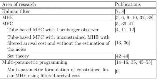
4.1 Estimation error and error set Ex for example 4.2, uncon-strained MHE and Kalman filter. . . 83
4.2 Estimation error and error setExfor example 4.3, constrained MHE. . . 86
4.3 Constrained error does not lie within the unconstrained error set. zoom into figure 4.2. . . 86
5.1 Error set Ex of unconstrained MHE and Kalman filter with error trajectory. . . 94
5.2 Explicit/multi-parametric solution of the robust tube-based MPC. . . 95
5.3 State trajectory starting from x1 = −0.6741, x2 = 3.551. x(τ), τ = 0, . . . ,12, mark the first 12 steps after start of sim-ulation. . . 95
5.4 Comparison between states and estimates of MHE and Kalman filter for robust and non-robust MPC. . . 96
5.5 Control action. . . 96
5.6 Error setEx for example 5.2, constrained MHE. . . . 98
5.8 Real value and estimates of statex2. . . 99
5.9 Noisew and v. . . 100
5.10 Explicit/multi-parametric solution of robust tube-based MPC. 100 5.11 Control action. . . 101
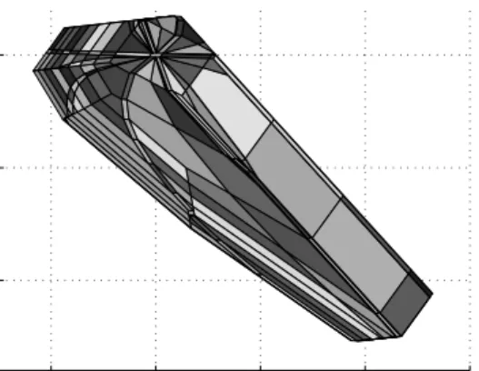
7.1 Three-layer control of UAVs. This thesis focuses on the gray areas. . . 108
8.1 Effect of non-holonomic constraints. . . 120
8.2 Example of a left-straight-left Dubins path. . . 123
8.3 A simple pursuit guidance (adopted from [2]). . . 127
8.4 Wind triangle. . . 127
9.1 Main elements of aircraft (with permission from NASA [3]). . 139
9.2 Roll, pitch, yaw, and body axes (with permission from NASA [3]). . . 141
9.3 NED inertial frame and body frame. . . 141
9.4 Angles in wing level flight. . . 143
9.5 Aerosonde over Tower Bridge. . . 153
10.1 Unstable open-loop. . . 156
10.2 Overview of the SAS. . . 157
10.3 Stability through the dampers. . . 159
10.4 Eigenvalues of all linearized models are nearly equal. . . 163
10.5 Comparison of non-linear and linear models, wind stepwx =7m/s.165 10.6 Comparison of non-linear and linear models, elevator step △δe= +1◦. . . 165
11.1 Overview over the 3-layer control structure. . . 168
11.2 Longitudinal guidance strategy. . . 170
11.3 Smoothing the change of altitude. . . 171
11.4 Left: lateral guidance strategy. Right: wind triangle. . . . 172
11.5 Simulation setup for three-layer control of the Aerosonde. . . 179
11.6 Yaw angle offset and oscillations. . . 180
11.7 The oscillations and the offset are removed due to the filter and the PID controller. . . 181
11.9 Setpoints and actual values. . . 182 11.10Control actions. . . 183 11.116m/s background wind from the east in inertial axes. . . 184 11.12Comparison of setpoints and actual values in 6m/s wind with
and without G. . . 184 11.13Horizontal flight path with variable altitude in 6m/s wind.
The x marks the point where the MPC becomes infeasible. . . 185 11.14Wind in body axes for flight with variable altitude in 6m/s
wind. . . 186 11.15Setpoints and actual values for flight with variable altitude in
6m/s wind. . . 186 11.16Control actions for flight with variable altitude in 6m/s wind. 187 11.17Horizontal flight path with constant altitude in 6m/s wind . . 188 11.18Wind in body axes for flight with constant altitude in 6m/s
wind. . . 188 11.19Setpoints and actual values for flight with constant altitude
in 6m/s wind. . . 189 11.20Control actions for flight with constant altitude in 6m/s wind. 189 11.2110m/s background wind in inertial axes. . . 191 11.22Horizontal flight path with variable altitude in 10m/s wind.
The x marks the point where the MPC becomes infeasible. . . 191 11.23Wind in body axes for flight with variable altitude in 10m/s
wind. . . 192 11.24Setpoints and actual values for flight with variable altitude in
10m/s wind. . . 192 11.25Control actions in 10m/s wind. . . 193 12.1 Horizontal flight path with constant altitude in medium wind. 199 12.2 Wind in body axes for flight with constant altitude in medium
wind. . . 199 12.3 Comparison of noise-free and noisy state measurements. . . . 199 12.4 Simulation setup for the different cases for wind estimation. . 200 12.5 Case 1.A: Wind estimate using the noise-free linear system,
all states measureable. . . 203 12.6 Case 1.B: Wind estimate using the noise-free linear system,
12.7 Case 1.C: Wind estimate using the noisy linear system, all
states measureable. . . 203
12.8 Case 1.C: Wind estimate using the noisy linear system, VA measurable. . . 203
12.9 Case 2.A: Wind estimate using the noise-free non-linear sys-tem, all states measureable. . . 204
12.10Case 2.B: Wind estimate using the noise-free non-linear sys-tem,VA measurable. . . 204
12.11Case 2.C: Wind estimate using the noisy non-linear system, all states measureable. . . 204
12.12Case 2.C: Wind estimate using the noisy non-linear system, VA measurable. . . 204
D.1 Flight path. . . 240
D.2 Angle of attack and sidelip angle. . . 240
D.3 Longitudinal and lateral states. . . 240
D.4 Flight path in 6m/s wind, variable altitude. . . 241
D.5 Angle of attack and sidelip angle in 6m/s wind, variable altitude.241 D.6 Longitudinal and lateral states in 6m/s wind, variable altitude.241 D.7 Flight path in 6m/s wind, constant altitude. . . 241
D.8 Angle of attack and sidelip angle in 6m/s wind, constant al-titude. . . 241
D.9 Longitudinal and lateral states in 6m/s wind, constant altitude.242 D.10 Angle of attack and sidelip angle in 10m/s wind. . . 242
nomenclature
Roman letters and abbreviations A state matrix
B input matrix C output matrix CR Critical Region
D direct transition matrix (state-space) Differential (controller)
d model mismatch e estimation error G disturbance matrix I Integral (controller)
KKT Karush-Kuhn-Tucker conditions of optimality LDI Linear Difference Inclusion
LPV Linear Parameter Varying LQR Linear Quadratic Regulator LTI Linear Time Invariant
MHE Moving Horizon Estimation/Estimation mp multi-parametric
MPC Model Predictive Control MPP Multi-Parametric Programming mRPI minimal RPI
N horizon length
P Proportional (controller)
PID Proportional Integral Differential (controller)
Q weighting matrix on states(MPC)/process noise(MHE)
Qy weighting matrix on outputs QP Quadratic Programming
RPI Robust Positively Invariant SS Steady-State u input vector v measurement noise w process noise x state vector y output vector
Subscripts and superscripts r, ref, s reference, setpoint
T−a|T value at t=T-a taken at time t=T
()∗ optimizer
ˆ
(·) estimated variable
ˆ
(·)∗ optimal estimated value of variable
(·)k|T value of variable at time k given or estimated at time T {·}Tk=i sequence from k=i to k=T
Sets
U⊕V Minkowski sum of sets Uand V
U∼V Pontryagin set difference of sets U andV U∪V union of sets Uand V
A≻0 A is positive definite
A0 A is positive semi-definite
co(A) convex hull ofA
kxk2Q kxk2Q,xTQx
Greek letters
Some of the default units are stated in spare brackets. All plots and values are in these units unless otherwise stated.
Roman letters and abbreviations AHRS Attitude Heading Reference System
AoA Angle of Attack AR Aspect Ratio
b wingspan
¯
c mean aerodynamic chord
CD drag coefficient
CD0 minimum drag coefficient of the airplane Cδa
D variation ofCD with aileron deflection [radians or degree]
Cδe
D variation ofCD with elevator deflection [radians or degree]
CDδf variation ofCD with flap deflection [radians or degree]
Cδr
D variation ofCD with rudder deflection [radians or degree]
CDM variation ofCD with Mach number
CL lift coefficient
CL0 zero-alpha lift: lift coefficient at zero AoA CLα alpha derivative: variation ofCL with AoA
CLα˙ α˙ derivative: variation of CL with the time derivative of the AoA
Cδe
L variation ofCL with elevator deflection
CLδf variation ofCL with flap deflection
CLq variation ofCL with the pitch rate
Cl rolling-moment coefficient
Clβ variation ofCl with sideslip angle
Clδa variation ofCl with aileron deflection
Cδr
l variation ofCl with rudder deflection
Clp variation ofCl with the roll rate
Clr variation ofCl with the yaw rate c.m. center of mass
Cm pitching-moment coefficient
Cm0 zero-alpha pitch: pitch moment at zero AoA Cα
m variation ofCm with AoA
Cmα˙ variation ofCm with the time derivative of the AoA
Cmδe variation ofCm with elevator deflection
Cmδf the variation ofCm with flap deflection
CmM variation ofCm with the Mach number
Cmq variation ofCm with the pitch rate
Cn yawing-moment coefficient
Cnβ variation ofCn with sideslip angle
Cnδa variation ofCn with aileron deflection
Cδr
n variation ofCn with rudder deflection
Cnp variation ofCn with the roll rate
Cnr variation ofCn with the yaw rate
CSF side force coefficient
CSFβ variation ofCSF with sideslip angle
Cδa
SF variation ofCSF with aileron deflection
CSFδr variation ofCSF with rudder deflection
CSFp variation ofCSF with the roll rate
Cr
SF variation ofCSF with the yaw rate
CX aerodynamic force in body x-axis
CY aerodynamic force in body y-axis
CZ aerodynamic force in body z-axis
D Drag
DCM Direction Cosine Matrix DoF Degree Of Freedom e efficiency factor EOM Equations Of Motion
Faero aerodynamic force
Fprop force due to propulsion GPS Global Positioning System
Hframe2
frame1 orthonormal transformation from frame1 to frame2
g gravity
h altitude [m]
LB
E,LEB non-orthonormal transformation from
L Lift
rolling moment
m mass
M pitching moment M Mach number
Maero aerodynamic moment
Mprop moment due to propulsion n load factor
N yawing moment
p roll rate in body axes [radians/s or degree/s] q pitch rate in body axes [radians/s or degree/s]
¯
q dynamic pressure
r yaw rate in body axes [radians/s or degree/s] S reference area of wing
SAS Stability Augmentation System SF Side Force
T Thrust
TAS True Air Speed
u inertial velocity alongxB [m/s] UAV Unmanned Aerial Vehicle
v velocity vector: frame specified by subscript v1 inertial velocity alongxI [m/s]
v2 inertial velocity alongyI [m/s]
v3 inertial velocity alongzI [m/s]
V Velocity: frame specified by subscript [m/s] A: TAS in body axes
v inertial velocity alongyB [m/s] w inertial velocity alongzB [m/s]
w wind [m/s]
W weight of the aircraft x Cartesian coordinate [m]
state vector
y Cartesian coordinate [m] z Cartesian coordinate [m]
Greek letters
α alpha AoA [radians or degrees]
β beta sideslip angle [radians or degrees]
δa delta aileron deflection [radians or degrees]
δe elevator deflection [radians or degrees]
δf flap deflection [radians or degrees]
δr rudder deflection [radians or degrees]
δth throttle setting, 0:closed, 1:fully open
ǫ epsilon induced drag factor
γ gamma flight path angle [radians or degrees]
µ mu bank angle [radians or degrees]
ω omega velocity vector in body axes
Ω Omega rotations/s of the propeller
φ phi roll angle [radians or degrees]
ψ psi yaw angle [radians or degrees]
ρ rho density
Θ Theta body attitude vector
θ theta pitch angle [radians or degrees]
ξ xi heading angle [radians or degrees]
Subscripts and superscripts A Air-relative frame
B Body frame
D Drag quantity related to drag g gust
I Inertial frame
L Lift quantity related to lift r reference, set-point
SF Side Force quantity related to side force T Thrust quantity related to thrust V Velocity frame W Wind frame WP WayPoint x in x-direction y in y-direction z in z-direction
Estimation techniques are vital for obtaining information about a system’s state and condition, for example to detect if a tank is leaking, but also for realising control of a system based on the state information [4–6]. The pur-pose of estimation is hence often to reconstruct this state information from a possibly noisy set of measurements. A long existing model-based technique for state estimation is the Kalman filter [7, 8], which is an unconstrained method. The use of constrained estimation techniques such as the moving horizon estimator (MHE) can lead to significant improvements of the esti-mation result [6, 9] by adding system knowledge, such as the fact that a leak is always an outflowing stream. MHE is an estimation method that obtains the estimates by solving a constrained optimization problem given a number,
orhorizon, of past measurements. It not only obtains the state information
but also the noise sequence over the horizon for the system [5, 6]:
xk+1 =Axk+Buk+Gwk
yk=Cxk+vk
(1.1)
where A is the system matrix, B the input matrix, C the output matrix andG captures the effect of the disturbancew wherew andv are assumed independent zero-mean Gaussian variables,xis the state vector,ythe output vector or measurement vector. The MHE hence differs from the Kalman filter in two important points [5, 6]:
1. Handling of constraints that potentially improves the estimation result significantly by incorporating system knowledge such as non-negativity of a leak [6] or re-present non-Gaussian noise [10].
2. Estimation not only of the state valuesxbut also of the values of the disturbance w over the horizon.
The obtained estimates can then be used for the control of the system using model predictive control (MPC), which is a model-based control method
that solves a constrained optimization problem to obtain the optimal control action to fulfill the purpose of the system, for example a certain quality of the final product for as little production cost as possible. The main advantages of MPC are the handling of multiple-input-multiple-output systems and the handling of system constraints that, for example, represent limitations to guarantee the safety of the system.
The objectives of this thesis are to investigate the use of linear MPC and linear estimation techniques in the following two parts:
Part 1: Simultaneous explicit/multi-parametric constrained moving horizon estimation and robust model predictive control.
Part 2: Multi-layer control of small unmanned aerial vehicles and in-flight wind estimation.
Part 1: Simultaneous explicit/multi-parametric constrained moving horizon estimation and robust model predictive control Estimation techniques are often embedded in a control structure that relies on the estimated values, such as model predictive control (MPC) [5]. MPC solves a constrained optimization in real-time to obtain the best control action and requires the current state information which can often not be measured directly but is only available as the result of an estimator. If noise is present in the available measurements there will inevitably be an error in the estimator’s results. If the controller and the estimator of the sys-tem are unconstrained, they can be designed independently without loss of optimality, following the separation principle. This principle does however not hold any more for constrained systems as the estimation error might significantly decrease the performance or lead to instability [5]. The con-strained MPC should hence not simply assume that the estimated values are correct but needs to consider the estimation error in order to obtain the best performance [5].
The consideration of the estimation error leads to robust control tech-niques such as tube-based MPC [4] that explicitly account for the measure-ment noise and the estimation error. Tube-based MPC requires the knowl-edge of how big the estimation error can become. While the determination of this error set is rather straight forward for unconstrained estimators such as the Luenberger observer [4, 11, 12] or the unconstrained MHE [13], no
significantly better estimates than unconstrained methods, the controller based on those better estimates will also perform better [5].
Model predictive control needs to solve the involved optimization problem in order to control the system. This means that the optimization problem needs to be solved frequently over and over again on-line while the system is under the control of the MPC. Multi-parametric programming is a method for solving constrained optimization problems that depend on some param-eters (for MPC they are for example the values of the current system state) over the range of parameters that is of interest for the problem. For MPC, multi-parametric programming can be used to derive the governing control laws for the system as a set of explicit functions of the system states off-line before the MPC control starts. It is hence a popular method for MPC be-cause it reduces the on-line computation time significantly [14–16]. Up to now, however, the constrained MHE and robust MPC have not been solved simultaneously via multi-parametric programming so that the computational advantage of this method cannot be realised.
Theobjectives of the first part of the thesis are
1. Derivation of a method to obtain the error set of the constrained MHE so that a robust controller can benefit from the better estimates. 2. Derivation of the estimation error and bounding error set of the
Kalman filter.
3. Derivation of a framework for the simultaneous design of explicit/ multi-parametric constrained MHE and robust tube-based MPC. 4. Derivation of the multi-parametric solution of the constrained MHE
and the tube-based MPC.
Part 2: Multi-layer control of small unmanned aerial vehicles and in-flight wind estimation
Unmanned Aerial Vehicles (UAVs) have recently attracted attention in re-search due to their numerous applications where direct human intervention is undesirable for safety reasons in hostile, hazardous, and geometrically complex environments, or in long-term monotonous missions [17–22]. The
goal in particular for long-term monotonous missions is to make the flight of the UAV as autonomous as possible to reduce the work-load of a remote human pilot [20]. Autonomous control of unmanned aerial vehicles is an disciplinary task of considerable complexity as a large number of inter-dependent design and implementation decisions have to be made [23]. A standard control structure consists of three layers [24, 25]: 1) the path plan-ner, 2) the guidance, and 3) the autopilot. The task of layer 1 is to plan a flight path for the aircraft such that mission objectives are accomplished. The task of layer 2 is to generate commands for the autopilot such that the planned flight path is followed. The task of layer 3, the autopilot, is to fly the aircraft such that it follows the guidance command but also such that flight safety is ensured at all times. The main issues in the control of small UAVs are [23, 26]:
• Guaranteeing safe flight such that safety constraints are not violated. • Inter-dependence and cross-effects of each part of the control structure. • Handling and estimation of wind.
Many of the difficulties in the control of small UAVs stem from wind. Small UAVs are prone to wind because of their light weight and low speed [27]. The wind is hence a disturbance that needs to be considered at each part of the control structure. The difficulty is that the wind cannot be predicted precisely enough through weather forecasts [28]. A method for in-flight wind estimation is hence needed. This part will investigate linear estimation tech-niques, in particular the Kalman filter as a benchmark and the MHE. The MHE will be investigated because it can inherently estimate disturbances. Model predictive control is an obvious choice for the autopilot because it can handle the flight safety constraints inherently. The objective of this thesis is to investigate how the wind can be incorporated in the model of the aircraft and hence in the MPC such that the autopilot ensures safe flight in windy conditions.
Theobjectives of the second part of the thesis can be summarized as follows:
1. Investigation of the cross-effects of each part of the control structure, in particular in the presence of wind.
2. Investigation of linear MPC for flight control.
3. Investigation of wind handling and wind estimation techniques.
1.1 Thesis outline
This thesis is split into two parts, where chapters 2 to 6 are dedicated to the first part and chapters 7 to 13 are dedicated to the second part. Due to the complex and diverse nature of each part, they are treated as complete entities with separate introductions and conclusions. General conclusions and future work related to the whole thesis are summarized in chapter 14. The detailed outline is as follows.
Part 1: Simultaneous explicit/multi-parametric constrained moving horizon estimation and robust model predictive control Chapter 2 provides an introduction to the simultaneous design of constrained MHE and robust MPC. Chapter 3 provides a literature overview of MHE, MPC, and multi-parametric programming. In chapter 4 the explicit/multi-parametric solution of the MHE is formulated and is then used to derive the error dynamics of the constrained linear MHE. Methods for calculating the bounding error sets of the MHE are also investigated. In the same chapter, the error dynamics and the calculation of the error set for the Kalman filter are presented. These error sets are then used in chapter 5 for the simultaneous design of explicit MHE and robust MPC. The work of the first part is validated by confirming that the Kalman filter and the unconstrained MHE give the same results. The conclusions and future work are outlined in chapter 6. Appendix A gives further details for the first part of the thesis.
Part 2: Multi-layer control of small unmanned aerial vehicles and in-flight wind estimation
Chapter 7 provides an introduction to the control of UAVs. Chapter 8 gives a literature overview of various aspects of flight control such as path planning, guidance, the design of autopilots, and wind estimation. The non-linear aircraft model of the system is described in chapter 9 and a discussion of relevant limitations of the aircraft’s flight capabilities is included. Since
the model predictive controller used in this work requires a linear model, linearization of the aircraft model is highlighted in chapter 10. Details about the setup of the three-layer control structure are given in chapter 11. In the same chapter, simulation studies are performed and discussed. In chapter 12, the Kalman filter and the linear moving horizon estimator are investigated for in-flight wind estimation. The findings in chapters 11 and 12 contain the novelties of the second part and determine the course of the future work as detailed in chapter 13. Appendices B to D give further details for the second part of the thesis. [29–34]
1.2 Financial support
This work was supported by the Engineering and Physical Sci-ences Research Council (EPSRC) of the United Kingdom (Grants EP/E047017/1 and EP/G059071/1) and by the European Research Council (MOBILE, ERC Advanced Grant No:226462). The sec-ond part was also supported by the Amelia Earhart Fellowship from Zonta International awarded in 2008 (http://www.zonta.org/WhatWeDo/ InternationalPrograms/AmeliaEarhartFellowship.aspx).
moving horizon estimation and
model predictive control
constrained moving horizon
estimation and robust model
predictive control
Model predictive control (MPC) is a model-based control technique that solves an optimization problem to derive the optimal control action in or-der to achieve the purpose of the system, for example the production of a product at minimum cost while guaranteeing its quality. The under-lying optimization problem needs to be solved at frequent intervals over and over again while the MPC controls the system. One popular approach to avoid the frequent solution of the optimization problem is to use multi-parametric programming. The key idea of explicit/multi-multi-parametric MPC is to solve the online optimization problem involved in a traditional MPC framework with multi-parametric programming and derive the control inputs as a set of explicit functions of the system states i.e. to obtain the governing control laws for the system at hand [14–16, 35]. The main advantage of explicit/multi-parametric MPC is that it replaces the online optimization-based implementation of traditional MPC with simple function evaluations which are faster than solving the optimization problem [16]. The imple-mentation of explicit/multi-parametric MPC, and generally MPC, relies on the assumption that the state values are readily available from the system measurements.
In reality however, the system measurements do not produce this infor-mation directly - instead the state inforinfor-mation needs to be inferred from the available output measurements with the use of a state estimator which obtains an estimatexˆ of the real state x. The controller and the estimator cannot be designed separately for constrained control applications because separation principle does not hold as the estimation error can significantly
degrade the controller performance or result in constraint violations [5]. This can be seen by the MPC problem of a linear discrete-time system with state and input constraints:
min uk k xNM P Ck 2 PM P C+ NM P C X k=1 kxkk2QM P C+ NM P C−1 X k=0 kukk2RM P C s.t. xk+1=Axk+Buk, x0 =x, (2.1) xk∈X,{xk∈Rn|Dxxk ≤dx}, uk∈U,{uk∈Rm|Duuk≤du}.
wherexand uare the states and inputs of the system,XandUare the sets
of the state and input constraints that contain the origin in their interior,
QM P C 0, PM P C 0 are symmetric positive semi-definite matrices and
RM P C ≻ 0 is a symmetric positive definite matrix, NM P C is the horizon length of the MPC, andkzk2
Q,zTQz.
The state estimatexˆreplaces the unknown real value ofxin (2.1) to obtain the control variable u. However, due to the estimation error ex = x−xˆ, the state constraints for the real system are described by Dx(ˆx+ex) ≤dx if the estimation error is bounded. It is obvious then that variations of the estimation error may result in constraint violations and that the effect of the estimation error ex has to be explicitly accounted for. In order to address the problem, the estimation and the control designs of the system have to be addressed simultaneously. Robust MPC methods such as tube-based MPC that ensure that the constraints of the system are not violated due to the presence of the estimation error can be employed if the bounds on the estimation error are known. In order to calculate these bounds, the dynamics of the error have to be known. The methodology proposed in this thesis addresses the problem of simultaneous estimation and control design. In order to achieve this, the following three steps need to be addressed:
1. Obtaining the dynamics that govern the estimation error (chapter 4.3), 2. Investigating methods for calculating the bounds on the estimation
error from the obtained error dynamics (chapter 4.4), and
3. Incorporating the error bounds into tube-based MPC that robustifies the system and the controller against the estimation error (chapter 5).
Previous work on this problem has focused on unconstrained estimators such as the Luenberger observer [4] and the unconstrained moving horizon estimator (MHE) [13, 36] but the Kalman filter constrained estimators have not yet been addressed.
Moving horizon estimation is a class of estimation methods in which the system state and disturbance estimates are obtained by solving a constrained optimization problem. This makes it possible to incorporate knowledge about the system into the constraints to improve the result of the estimation. These constraints may represent system properties such as non–negativity of an inflowing liquid or may account for non–zero–mean noise of the sensors and hence significantly improve the estimates [5, 6, 9].
2.1 Objectives and contributions of this thesis
The objectives of this thesis are to close some gaps in linear control and esti-mation. The main focus of this thesis is placed on the simultaneous design of constrained MHE and tube-based MPC so that the better estimation result of the constrained estimator can be used for robust control. The objectives and contributions of this thesis in detail are:
• Derivation of the error dynamics and bounding sets of the estimation error for the Kalman filter and the constrained MHE.
• Design of robust tube-based MPC using the Kalman filter and con-strained MHE.
• Formulation of the explicit/multi-parametric solution of constrained MHE and the tube-based MPC.
2.2 Outline
Chapter 3 gives a literature overview of MHE, MPC, including robust tube-based MPC and the required set calculations, and multi-parametric pro-gramming. In chapter 4 the explicit/multi-parametric solution of the MHE is formulated and the error dynamics of the linear Kalman filter and the constrained MHE are derived. In the same chapter methods for calculating the bounding error sets for the Kalman filter and the unconstrained and the
constrained MHE are discussed. The obtained error sets are then used in chapter 5 for the simultaneous design of explicit MHE and robust tube-based MPC. The results are validated by comparing the Kalman filter and the un-constrained MHE. Finally, chapter 6 draws conclusions and outlines future work. In appendix A further details for the derivation of the MHE, the calculation of mRPI sets, and the algorithm for quadratic multi-parametric programming are presented.
2.3 Publications
1. A. Voelker, K. Kouramas, and E. N. Pistikopoulos, “Simultaneous state estimation and model predictive control by multi-parametric program-ming,” in 20th European Symposium on Computer Aided Process
En-gineering, Ischia, Naples, Italy, 2010.
2. A. Voelker, K. Kouramas, and E. N. Pistikopoulos, “Unconstrained moving horizon estimation and simultaneous model predictive control by multi-parametric programming,” in UKACC International
Confer-ence on Control, Coventry, UK, 2010, pp. 1154–1159.
3. A. Voelker, K. Kouramas, and E. N. Pistikopoulos, “Simultaneous con-strained moving horizon state estimation and model predictive control by multi-parametric programming,” in 49th IEEE Conference on
De-cision and Control, Atlanta, Georgia, USA, 2010, pp. 5019–5024.
4. A. Voelker, K. Kouramas, and E. N. Pistikopoulos, “Simultaneous De-sign of Explicit/Multi-Parametric Constrained Moving Horizon Esti-mation and Robust Model Predictive Control” in Automatica, submit-ted 2011
MPC
This chapter provides the theoretical background necessary for the simulta-neous design of a state estimator and an explicit robust tube-based model predictive controller (MPC). An overview of the literature related to Kalman filtering, moving horizon estimation (MHE), MPC in general, and tube-based MPC in particular is given. Additionally, the set-theoretical concepts that are employed in tube-based MPC are briefly introduced. Finally multi-parametric programming which can be used to derive an explicit solution of the MHE and the MPC is introduced. Table 3.1 summarizes the literature in these areas and shows the structure of this chapter.
Area of research Publications
Kalman filter [7, 8]
MHE [5, 6, 9, 10, 37, 38]
MPC [5, 39–41]
Tube-based MPC with Luenberger observer [4, 11, 12] Tube-based MPC with unconstrained MHE with
filtered arrival cost and without the estimation of the noise
[13, 36]
Set theory [42–44]
Multi-parametric programming [14–16, 35, 45–53] Multi-parametric formulation of constrained
lin-ear MHE using filtered arrival cost [9]
Table 3.1: Literature related to estimation, MHE, multi-parametric program-ming, and robust explicit MPC.
The following discrete-time linear system is considered in the first part of this thesis:
xk+1 =Axk+Buk+Gwk (3.1)
whereA is the system matrix,B the input matrix,C the output matrix,G
captures the effect of the noisew. The additive noise wand v are assumed independent zero-mean Gaussian variables (Markov process). x is the state vector, y the output or measurement vector. The dimensions of the ma-trices and vectors are: x ∈ Rn×1, A ∈ Rn×n, u ∈ Rm×1, B ∈ Rn×m, y ∈ Rp×1, C ∈ Rp×n, w ∈ Rq×1, G ∈ Rn×q, v ∈ Rr×1. The following
assump-tion about the system holds for the work of this thesis: Assumption 3.1
• The system (A, C) is observable.
• The noise v, w is bounded in the polytopic sets v ∈ V and w ∈ W
containing the origin in their interiors.
3.1 The Kalman filter
The linear Kalman filter is a standard method for unconstrained state es-timation for the system (3.1) - (3.2) and is a common benchmark for com-parison with other estimators [5–8]. It will also be used in this thesis for comparison with the moving horizon estimator. This section gives only a very brief overview and more details can be found in the related literature. The Kalman filter follows a two-step procedure to calculate the maximum a-posteriori Baysian estimate [7, 8]. The first step is the time update, the second step is the measurement update. The first step uses the system model to predict the current state of the system based on the last estimate. In the measurement step this prediction is updated by using the sensor informa-tion. The Kalman filter is hence a predictor-corrector type estimator that is optimal in the sense that it minimizes the estimated error covariance [8]. The Kalman filter for system (3.1) - (3.2) is given by [8]:
1) Time update/ prediction step/ a-priori: Prediction of the state:
ˆ
xk|k−1 =Axˆk−1|k−1+Buk−1,
Projection of the error covariance:
Pk|k−1 =APk−1AT +Qkal.
2) Measurement update/ correction step/ a-posteriori: Computation of the Kalman gain:
Kk=Pk|k−1CT(CPk|k−1CT +Rkal)−1, Update of the estimate with the measurement:
ˆ
xk|k= ˆxk|k−1+Kk(yk−Cxˆk|k−1),
Update of the error covariance:
Pk= (I−KkC)Pk|k−1.
(3.4)
where Qkal and Rkal present the measure of confidence in the model and the measurement. The larger the entries inRkal are in relation toQkal the more relative trust is put into the measurements over the system model. The solution of the discrete algebraic Riccati equation [7]
P =ATP A−ATP B(BTP B+Rkal)−1BTP A+Qkal (3.5) can be used for the calculation of the steady-state gain which makesPk+1 = Pk=P constant.
3.2 Moving horizon estimation
The Kalman filter considers only one set of measurements at a time. In [5] is shown that the Kalman filter is the algebraic solution to the following unconstrained least-square optimization problem:
min ˆ x0,{wˆ}Tk=0−1 =kxˆ0−x0k2P−1 0 + T−1 X k=0 kwˆkk2Q−1 k + T X k=0 kˆvkk2R−1 k (3.6) where ˆ xk+1 =Axˆk+Buk+Gwˆk ˆ yk=Cxˆk+ ˆvk
andQk≻0,Rk≻0,P0 ≻0are positive definite matrices and x0 is the mean
of xˆ0. This optimization problem now opens the possibility to add system
knowledge in the form of constraints. The constraints might for example capture the fact that a leak is always an outflowing stream or account for
non-zero non-Gaussian noise [10]. The optimization problem (3.6) is then not equivalent to the Kalman filter any more. If all the available past mea-surements are used for the estimation as in (3.6), the estimation problem grows unbounded with time. This is referred to as the full information
es-timator [6]. A probabilistic derivation of the full information estimator can
be found in appendix A.1. The derivation is based on the maximization of the a-posteriori Baysian estimate. In order to keep the estimation prob-lem computationally tractable it is necessary to limit the processed data, for example by discarding the oldest measurement once a new one becomes available. This essentially slides a window over the data, leading to the
mov-ing horizon estimator(MHE). The data that is not considered any more can
be accounted for by the so calledarrival cost so that the information is not lost (see section 3.2.1). The MHE then considers only a limited amount of data so that the constrained optimization problem becomes:
min ˆ xT−N|T,WˆT kxˆT−N|T −xT−N|Tk2 PT−−1N|T−1− kYTT−−N1 − OxˆT−N|T −cb U¯ TT−−N2k2W−1+ T−1 X k=T−N kwˆkk2Q−1 k + T X k=T−N kˆvkk2R−1 k (3.7) s.t. xˆk+1 =Axˆk+Buk+Gwˆk, yˆk =Cxˆk+ ˆvk, ˆ xk ∈Xˆ ,{xˆk∈Rn|Dˆxxˆk≤dˆx}, ˆ wk∈Wˆ ,{wˆk∈Rq|Dˆwwˆk≤dˆw}, (3.8) ˆ vk∈Vˆ ,{vˆk∈Rr|Dˆvvˆk ≤dˆv},
where T is the current time, Qk ≻ 0, Rk ≻ 0, PT−N|T−1 ≻ 0 are the
covariances of wk, vk, xT−N assumed to be symmetric, N is the horizon length of the MHE, i.e. the amount of past data taken into account. YT
T−N =
[yTT−N, . . . , yTT]T is a vector containing the pastN+1measurements,UTT−−N1 = [uTT−N, . . . , uTT−1]T is a vector containing the past N inputs. x,w,v denote the variables of the system (3.1)-(3.2). xˆ,wˆ,ˆvdenote the estimated variables of system (3.8), and xˆ∗T|T−N and Wˆ∗
T = WTT−−1N
∗
= {wˆ}TT−|T1−N∗ denote the optimizers of problem (3.7)–(3.8) whereWˆT =WTT−−N1 ={wˆ}TT−|T1−N denotes the estimated noise sequence from time T −N to time T −1. Finally,
kxˆT−N|T−xT−N|Tk2
PT−−1N|− kT−1Y T−1
T−N− OxˆT−N|T −cb U¯ TT−−N2k2W−1 is the arrival
cost which will be discussed in section 3.2.1 and is given in equation (3.11). For steady-state MHE Qk = Q, Rk = R, and PT−N|T−1 = P are
time-invariant.
The current state of the system can be calculated from the initial state
xT|T−N by forward programming using the system equations (3.1) and (3.2) if the deterministic inputUTT−−N1 and the noise sequence{w}TT−−1N are known. It is thus sufficient to estimate the initial state xˆ∗T|T−N and the noise Wˆ∗
T. The concept of MHE is illustrated in figure 3.1 where (·)T−k|T denotes the sample at timeT−kobtained at time T.
time T −N T estimation horizon measured outputsyT−k|T future past T −1 noise sequence {wˆ}TT−−1N T s ˆ xT−N|T ˆ xT inputs uT−k|T
Figure 3.1: Concept of moving horizon estimation. The MHE is applied with the following steps:
1. The optimization problem (3.7) - (3.8) is solved to obtainxˆ∗T|T−N and
ˆ
W∗
T.
2. The current state estimate xˆ∗
T|T is obtained by substituting xˆ∗T|T−N and Wˆ∗
T into the system dynamics xˆk+1 = Axˆk +Buk +Gwˆk and projecting the state values forward from time T −N to the current time T byxˆ∗
T|T =ANxˆ∗T−N|T +
PT−1
j=T−NAT−1−jGwˆj∗
3. When the next measurement becomes available (at the next sampling instance), steps 1 and 2 are repeated.
Remark 3.1 In the case T ≤ N, the full information estimator is solved
using the arrival costkxˆT−N|T −xT−N|Tk2
P0−1. The horizon ‘fills up’ and no
Remark 3.2 Rao [6] points out that wrongly posed constraints might lead
to an infeasible optimization problem and that hard constraints on ˆvk could
be problematic due to the possibility of outliers in the measurement. Any
constraints posed in (3.8) should hence be chosen such that the real system
does not violate them [6].
This observation leads to the following assumption for the work in this thesis: Assumption 3.2 The real system does not violate the constraints posed to
the MHE:x∈Xˆ, v∈Vˆ, w∈Wˆ which contain the origin in their interior.
The potential improvement of the state estimate by posing constraints is demonstrated in example 3.1 [6]. In this example the constrained MHE and the Kalman filter are compared for the linear system (3.9). The simulation depicted in figure 3.2 clearly shows the improvement of the constrained MHE compared to the Kalman filter where the MHE better approximates the real state while the Kalman filter gives a poorer estimate.
Example 3.1 xk+1 = " 0.9962 0.1949 −0.1949 0.3815 # xk+ " 1 1 # uk+ " 0.03393 0.1949 # wk, yk= [1 −3]xk+vk, (3.9) ˆ wk∈Wˆ ,{wˆ∈R| −0.01≤wˆ},W.
3.2.1 Different update schemes of the arrival cost
The MHE can only consider a limited amount of past data while remaining computationally tractable. The information in the discarded data should not be simply ‘thrown away’, but preserved. This is achieved through the arrival cost which captures the older data through forward dynamic programming. It can hence be seen as an equivalent to thecost to go in backward dynamic programming [6]. In the constrained case, the arrival cost cannot be calcu-lated analytically [6]. Rao [6] argues that the unconstrained arrival cost is a reasonable choice because it is exact if no constraint is active. Caution needs to be taken because an ill-chosen arrival cost can lead to an unsta-ble estimator [6], but in [6] it is also shown that the steady-state (constant
PT−N|T−1) constrained estimator is stable if PT−N|T−1 ≥ P∞ where P∞
is the solution of the discrete algebraic Riccati equation (3.5) (see section 3.2.3). The arrival cost needs to be updated at each time step and Findeisen [37] and Rao [6] suggest two different update schemes for xT−N|T:
1. Filtered update scheme [6, p. 74]: Use of the optimal estimate xT−N|T =
Axˆ∗T−N−1|T−N−1+BuT−N−1|T−N−1 +Gwˆ∗T−N−1|T−N−1 N + 1 time steps in the past.
2. Smoothed update scheme [6, p. 83]: Use of the optimal estimate from the last time step xT−N|T = Axˆ∗T−N−1|T−1 +BuT−N−1|T−1 +
GwˆT∗−N−1|T−1.
Rao [6] demonstrates that either update can give a better estimate than the full-information estimator if the estimation constraints (3.8) are not properly posed and the real system violates them but no general claim about robustness is made. The MHE with the smoothed update performs best but further research in this direction still remains open. The main disadvantage of the filtered update is that cycling effects can occur because the filtered update can be seen as N independent parallel running filters [6, 37]. The use of the smoothed update however avoids the cycling effect and hence this work only considers the smoothed update. The smoothed arrival cost is calculated as follows [38]:
kxˆT−N|T −xT−N|Tk2
PT−−1N|T− k−1Y T−1
where fori, j ≤N O=hCT ATCT . . . A(N−1)TCTiT , Mi,j = 0 if j≥i, C G if j=i−1, C Ai−1Ai−2 . . . Aj+1G otherwise, (3.11) W =diag(R) +Mdiag(Q)MT
andPT−N|T−1is calculated by the following backward Riccati equation [38]:
Pk|T =Pk|k+Pk|kAT Pk−+11|k(Pk+1|T −Pk+1|k)Pk−+11|kA Pk|k,
Pk|k=Pk|k−1−Pk|k−1CT(R+C Pk|k−1CT)−1C Pk|k−1, (3.12)
Pk|k−1=G Q GT +A Pk−1|k−1AT.
3.2.2 Alternative formulations of the MHE
Apart from the MHE formulation stated in equation (3.7), a number of vari-ations in the formulation can be found in the literature which are mentioned here for reasons of completeness. Alessandri et al. [36] used the following objective function in which the estimates of the noise sequence WˆT are not
obtained: J = µkxˆT−N|T −xT−N|Tk2 +
PT
k=T−Nky(T)−Cxˆ(k|T)k2. In this formulation the scalar µ is used to guarantee stability. By reason of optimality, the formulation (3.7) will give at least as good a result as the formulation in Alessandri et al.. Darby and Nikolaou [9] introduced a non-zero meanwm,k for wˆk using the filtered update of the arrival cost:
min ˆ xT−N|T,WˆTT−−N1|T kxˆT−N|T −xT−N|Tk2 PT−−1N|T−N+ T−1 X k=T−N kwˆk−wm,kk2Q−1 + T X k=T−N kvˆkk2R−1 (3.13)
3.2.3 Stability of the MHE
The stability of the MHE is crucial in ensuring that a good estimate is obtained. Conditions for stability of the MHE have been studied in [6] and in this section the results which are relevant for this work will be presented.
Loosely speaking, stability is defined for the nominal, i.e. the noise-free, system (v = 0, w = 0) as follows: the filter converges from a wrong initial state to the actual state (asymptotic convergence) and the estimation error will remain zero for all future time once it is zero (simulator property). Mathematically this is expressed by the following definition:
Definition 3.1 [6, p. 75] The estimator is an asymptotically stable ob-serverfor the system
xk+1 =Axk, yk =Cxk
if for anyǫ >0 there corresponds a number δ >0 and a positive integer T¯
such that ifkx0−xˆ0k ≤δ andxˆ0∈X, thenkxˆT −ATx0k ≤ǫfor all T ≥T¯
andxˆT →ATx0 as T → ∞.
In corollary 4.5.3. in [6] the following stability conditions for the constrained, linear MHE using the smoothed arrival cost are stated:
Proposition 3.1 [6, p. 83] The constrained linear MHE with smoothed arrival cost is asymptotically stable if
1. Qk ≻0, Rk ≻0, P0 ≻0, PT−N|T−1≻0,
2. N ≥n,
3. (A, C) is observable, and
4. assumption 3.2 holds.
Stability of the MHE (3.7)-(3.8) for the nominal system is proved by the following steps, the details of which can be found in [5, 6, 37]:
1. Under the conditions of proposition 3.1, it is shown that the value function of (3.7) - (3.8) is monotonically non-decreasing.
2. It is shown that the value function is bounded above.
3. From this can be shown that the estimator converges and the estima-tion error goes to zero as T → ∞ and asymptotic stability is estab-lished.
3.2.4 Equivalence to the Kalman filter
The unconstrained linear MHE is equivalent to the linear Kalman filter if the solution of the differential algebraic Riccati equation (3.5) is used for P0 in the arrival cost of the MHE and in the Kalman filter [6, 37].
This equivalence will be useful for validating the results of this thesis in the subsequent chapters.
3.3 Model predictive control
The termmodel predictive control describes the basic underlying principle: a dynamic model of the system is used to forecast or ‘predict’ the behaviour of the system. The future control moves can be used to optimize the predicted behaviour of the system to obtain the optimal control moves such that the objective of the system is best fulfilled [5]. The objective might for example be to produce a product to a certain quality as cheaply as possible. The control moves are determined through an optimization problem where the objective of the system is represented by the objective function [5, 39–41]. The control task is posed as an optimization problem which allows the ex-plicit inclusion of constraints for example on the inputs, outputs, and states of the system. One basic formulation of the optimization problem based on state-space models is [5] whereys is the setpoint ony:
min uk k xNM P Ck 2 PM P C+ NM P C X k=1 kyk−ysk2QM P C+ NM P C−1 X k=0 kukk2RM P C s.t. xk+1 =Axk+Buk, yk=Cxk (3.14) xk∈X,{xk∈Rn|Dxxk≤dx}, uk∈U,{uk∈Rm|Duuk≤du}, yk∈Y,{yk∈Rp|Dyyk≤dy}.
The solution of this optimization problem depends on the current system state. The concept of MPC is depicted in figure 3.3. The repetitive nature of the basic steps for the implementation of a model predictive controller leads to an implicit feedback control [39]:
2. The optimization problem is solved to obtain a sequence of future control inputs.
3. The first control input out of this sequence is applied to the system. 4. When the next measurement becomes available the procedure is
re-peated from step 1.
time future past k k+ 1 k+m k+p control horizon prediction horizon predicted outputsyk+i|k sequence of inputsuk+i|k T s setpointys Figure 3.3: Concept of MPC.
The following comments highlight some of the issues related to the steps of the implementation:
1. The MPC (3.14) requires full state information in order to solve the optimization problem. If not all states of the system can be measured, a state estimator is needed to generate the missing values from the measurements. The estimation error might significantly decrease the performance of the MPC and needs to be taken into account to avoid constraint violations (see [5], the introduction of this part of the thesis, and section 3.3.6).
2. The optimization problem (3.14) uses a linear model of the system. This leads to a convex quadratic optimization problem which can quickly be solved to obtain its unique global optimum [5]. The performance of the MPC depends significantly on the quality of the model. Since a linear model represents the system completely only in simple or artificial cases, the linear model used in MPC normally captures the real system only with an error. The use of a non-linear model can hence improve the performance of the controller at extra computational cost because then a linear, often non-convex optimization problem has to be solved [5, 41]. Whereas there is a wide field of research for non-linear MPC [5], linear MPC is the dominant variety used in industry and there are still open problems related to linear control.
Hence, this thesis concentrates on some open issues in linear MPC, such as the simultaneous use of a linear tube-based MPC and a linear constrained MHE which has not yet been considered in the literature.
3. The control and prediction horizon can be of the same or different lengths where the control horizon cannot be longer. If it is shorter, some control strategy must be assumed for the remainder of the prediction horizon such as keeping the control input constant [5]. In the MPC formulation (3.14) the horizons are of the same length, in figure 3.3 their lengths are different. 4. In step 3, the first control input can be applied immediately once it be-comes available when the optimization problem has been solved, or at fixed time intervals. Applying it immediately might lead to better control perfor-mance while the application at fixed time intervals simplifies the analysis of the controller and the time delay can be taken into account when obtaining the control sequence [39]. In this thesis, the control input will be applied in fixed equidistant intervals.
5. Measurements of the system are normally not all available at the same time at the same rate. For simplicity of implementation, it is however often assumed that all measurements become available in fixed intervals (see figure 3.3). If this simplification affects the performance of the controller, it cannot be neglected [39]. It will be assumed in this thesis that all measurements are available synchronously at fixed equidistant interval and that this intervals is identical to the interval at which the control input is applied to the system.
3.3.1 Advantages of MPC
The success of MPC is based on two main advantages [40]:
1. The ability of handling multiple-input-multiple-output (MIMO) sys-tems and
2. The ability of handling (hard) constraints in the optimization problem. The model of the system can be obtained such that it relates multiple outputs to multiple inputs. Constraints can be included by simply adding them to the optimization problem. Theoretically, any kind of constraints can be in-cluded, often on outputs and inputs which represent the physical properties of the actuators or the quality of the product [39]. The direct considera-tion of the constraints allows the controller to operate the system close to
its boundaries which is often a necessity for optimal performance or max-imization of profit while quaranteeing to not violate the physical or safety constraints of the system [5, 40].
3.3.2 Disadvantages of MPC
The three main issues about MPC are [39, 40]:
1. The required computation time to solve the optimization problem, 2. The handling of the mismatch between the model used for the design
of the MPC and the real system, and
3. The possibility of the optimization problem becoming infeasible. The main disadvantage of MPC is that the solution of the underlying opti-mization problem might require considerable computation time [40]. MPC hence originated in the process industry where the systems are ‘slow’ and the required computation time is available. With faster computers and advances in optimization techniques, MPC can be applied to a growing area of ap-plications [39]. Optimization algorithms that exploit the structure of MPC are for example based on structured interior point methods [6] or on partial enumeration [54]. Another approach to reduce the computation time during the operation of the system is to solve the optimization problem with multi-parametric programming techniques (see section 3.4). Rather than solving the optimization problem repetitively on-line it is solved once off-line, before the start of the system to obtain the solution over the range of interest of the current state. The on-line solution then consists only of the evaluation of affine functions [15, 35, 45, 46, 50–52, 55].
The model of the system on which the design of the MPC is based does not, with the exception of simple or artificial examples, capture the be-haviour of the real system completely and precisely. A model mismatch is almost always present. This mismatch can be estimated and incorporated into the model [39] (see section 3.3.3). Due to this model mismatch, the MPC might predict constraint violations which do not exist in reality or predict none when violations actually occur. This affects the prediction of the states and the outputs, but not the inputs, since they are determined by the optimization and hence the MPC has direct control over the inputs [39].
Hence, it might be possible that the optimization problem becomes infeasi-ble, in which case no control inputs are calculated. Consequently there is the need for a strategy to avoid or handle this situation (see section 3.3.4). Treating some or all of the constraints as soft constraints that can be vio-lated if necessary rather than hard constraints is one approach to avoid an infeasible optimization problem [39] (see section 3.3.4). MPC methods that explicitly take the mismatch and other noise and disturbances into account are addressed with robust control methods [5] (see sections 3.3.4 and 3.3.6).
3.3.3 Handling of the model-mismatch
With the exception of simple and artificial cases, a model mismatch exists between the model used in the design of the MPC and the real system. In many cases the system dynamics are described by complex non-linear dynamics while a linear model is used for the MPC formulation. The model mismatch will affect the performance of the controller but methods exist that reduce the effect [39]. One such method is to incorporate the estimated model mismatch into the state-space system and hence improve the model which in turn leads to a better control performance:
xk+1 =A xk+B uk+G wk
yk =C xk+D uk+ek
(3.15)
where ek is the mismatch vector and k = 0, . . . , NM P C. In the simplest case it is assumed constant over the whole prediction horizon and can


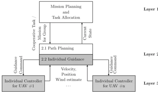
![Figure 9.1: Main elements of aircraft (with permission from NASA [3]).](https://thumb-us.123doks.com/thumbv2/123dok_us/473868.2556003/139.892.233.661.172.484/figure-main-elements-aircraft-permission-nasa.webp)

