Stopping Criterion for Boosting Based Data Reduction Techniques: from Binary to Multiclass Problem

Stopping Criterion

for Boosting-Based Data Reduction Techniques:

from Binary to Multiclass Problems

Marc Sebban [email protected]

Eurise, Faculty of Sciences University of Jean Monnet

42023 Saint-Etienne Cedex 2, France

Richard Nock [email protected]

GRIMAAG, Scientific Department French West Indies and Guiana University 97275 Schoelcher Cedex, Martinique, France

St´ephane Lallich [email protected]

ERIC, Department of Economics

University of Lyon 2, 69676 Bron Cedex, France

Editors: Carla E. Brodley and Andrea Danyluk

Abstract

So far, boosting has been used to improve the quality of moderately accurate learning algorithms, by weighting and combining many of their weak hypotheses into a final classifier with theoretically high accuracy. In a recent work (Sebban, Nock and Lallich, 2001), we have attempted to adapt boosting properties to data reduction techniques. In this particular context, the objective was not only to improve the success rate, but also to reduce the time and space complexities due to the storage requirements of some costly learning algorithms, such as nearest-neighbor classifiers. In that framework, each weak hypothesis, which is usually built and weighted from the learning set, is replaced by a single learning instance. The weight given by boosting defines in that case the relevance of the instance, and a statistical test allows one to decide whether it can be discarded without damaging further classification tasks. In Sebban, Nock and Lallich (2001), we addressed problems with two classes. It is the aim of the present paper to relax the class constraint, and extend our contribution to multiclass problems. Beyond data reduction, experimental results are also provided on twenty-three datasets, showing the benefits that our boosting-derived weighting rule brings to weighted nearest neighbor classifiers.

1. Introduction

Some of the earliest approaches to classification are also among the simplest: they do not induce concept representations (decision trees, neural networks, etc.), but exploit simple structures of the learning set, such as neighborhoods, to classify instances. Among them, the most popular is prob-ably the 1-Nearest-Neighbor (NN) algorithm (Cover and Hart, 1967), and its generalization, the

k-NN rule, which classifies an unknown instance according to a local vote by its k-nearest

the large-sample risk incurred is less than twice the Bayes risk. Even more, the risk paid off for finite samples can be very reasonable under similar assumptions (Nock and Sebban, 2001b). How-ever, from a practical point of view, this algorithm has several problems, as mentioned in Breiman et al. (1984): (i) it is computationally expensive because it stores all the instances in memory; (ii) it is intolerant to noisy instances; (iii) it is intolerant to irrelevant attributes and (iv) it is sensitive to the chosen distance function.

The deletion of noisy instances and irrelevant attributes is addressed by data reduction tech-niques. Recent complexity theoretic results show that some related optimization problems are very hard to approximate (Nock and Sebban, 2000). This advocates for the use of heuristics for data reduction. In this paper, we only focus on prototype selection, which consists of identifying and eliminating irrelevant instances. Prototype selection concerns both storage complexity (first prob-lem listed above) and noise tolerance (second probprob-lem). The last two probprob-lems are not discussed in this paper. Many solutions have been proposed to select relevant features (John, Kohavi and Pfleger, 1994; Koller and Sahami, 1996; Sebban, 1999) and to define new distance functions (Wilson and Martinez, 1997).

Many prototype selection methods have been suggested to improve the standard NN algorithm using different strategies: removing correctly classified examples (Hart, 1968; Gates, 1972), iden-tifying and eliminating mislabeled instances (Brodley and Friedl, 1996), deleting misclassified or irrelevant instances (Wilson and Martinez, 2000; Sebban and Nock, 2000), identifying relevant prototypes by Monte-Carlo sampling (Skalak, 1994), etc. Recently, we proposed an adaptation of

boosting to prototype selection (Nock and Sebban, 2001a) in the PSBOOST algorithm. Boosting,

as used in the well known ADABOOST algorithm (Freund and Schapire, 1997), generates a final

combined classifier whose error on the learning set is small by weighting and combining T weak hypotheses, each of which may have a large error. Here, T is the number of boosting rounds, a parameter fixed in advance. Freund and Schapire (1996) proposed reducing the number of instances used by each weak hypothesis to speed up the NN classifier. As far as we know, this work was the first attempt to use boosting in prototype selection, although their goal was not to improve the

accuracy. The objective of PSBOOSTis to obtain a good balance between storage requirements and

generalization accuracy. Its principle is to use each instance as a weak hypothesis: the confidence weight given by boosting becomes in our case an indication of the instance’s relevance. Experimen-tal results indicate the efficiency of this approach (Nock and Sebban, 2001a). Inspired by boosting, PSBOOSTsuffers from the same important drawback: the control of the number of boosting rounds,

that is, the size Np of the final prototype set in our framework. Nock and Sebban (2001a) studied

the balance between a small value of Npwhich allows high storage reduction but decreases the

ac-curacy, and a large value which allows us to control the generalization accuracy but still needs high storage requirements. The results obtained reveal the crucial need for a method fixing as accurately as possible this parameter (Nock and Sebban, 2001a). A first attempt to cope with this problem is provided by Sebban, Nock and Lallich (2001), but it holds only for problems with two classes.

In this paper, we relax the class constraint, thereby extending our framework to multiclass prob-lems. We draw up a statistical test based on the normalization factor Z, the criterion minimized in ADABOOST, and optimized in PSBOOST as well. Experimental results display the ability of this criterion to obtain a significant size reduction, together, on average, with an increase of the

accuracy. This generalized version of PSBOOST, called PSBOOST2 MC, also displays

A significant drawback of k-NN classifiers is that they require fixing k in advance. This is clearly not an easy task in real-world domains. While a small value of k is often sufficient for noise free problems, the k-NN rule requires thorough investigations for complex problems, often leading to the testing of many values of k. To cope with this problem, in this paper, we extend our algorithm to another kind of neighborhood-based classifier, whose geometry does not rely on ad hoc parameters. The underlying neighborhood graph is called the Relative Neighborhood Graph (RNG) (Toussaint, 1980). Experimental results again display the ability of our algorithm to improve classifiers based on the RNG, even in the presence of noise.

The final contribution of this paper is not restricted to data reduction. In Sebban, Nock and Lallich (2001), it is argued that the instance’s weighting rule derived from boosting deserves inves-tigations for its use in weighted nearest neighbors classifiers. We provide in this paper experimental results on a body of twenty-three datasets. They display significant improvements obtained when using boosting-derived weights.

In the rest of this paper, after having briefly recalled the main properties of boosting and

PS-BOOST in Section 2, we describe in Section 3 our statistical criterion for automatically halting the

selection procedure, and the new version of our algorithm, called PSBOOST2. In Section 4, we

describe the RNG, before presenting a large experimental study (Section 5). We make some obser-vations in Section 6, and we explain why PSBOOST2 is suited for reducing storage while controlling

the classifier accuracy. In Section 7, we present the extension of the test to multiclass problems. The use of the instance weights in weighted classifiers is discussed in Section 8, before our final conclu-sion.

2. Adapting Boosting to Data Reduction

In this section, we recall the main properties of boosting and PSBOOST.

2.1 Properties of Boosting

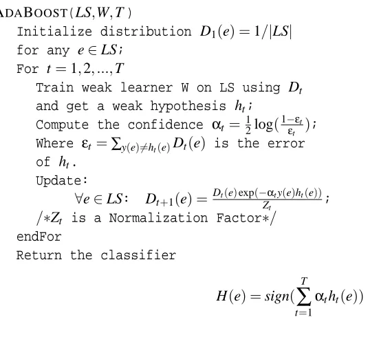
Boosting resides in combining many (T ) weak hypotheses produced from various distributions

Dt(e) over the learning set (LS). The pseudocode of the original boosting algorithm, called AD

-ABOOST (Freund and Schapire, 1997) is described in Figure 1. At each stage t, ADABOOST

de-creases (resp. inde-creases) the weight of learning instances, a priori labeled y(e), which are correctly

(resp. incorrectly) classified by the current weak hypothesis ht. Boosting thus forces the weak

learner to learn the hardest examples. The weighted combination H(e)of all the weak hypotheses

results in a better performing model. Schapire and Singer (1998) proved that, in order to mini-mize learning error, one must seek to minimini-mize Zt in each round of boosting, requiring the use of a

specific confidenceαt.

In order to present our adaptation of boosting to storage reduction with neighborhood-based classifiers, we first introduce several notations proposed by Schapire and Singer (1998). Suppose that y(e)∈ {−1; 1}and that the output of each weak hypothesis ht is restricted to−1,0,+1. Let W−1, W0and W+1be defined by

Wb =

∑

e∈LS:y(e)ht(e)=b

ADABOOST(LS,W,T)

Initialize distribution D1(e) =1/|LS| for any e∈LS;

For t=1,2,...,T

Train weak learner W on LS using Dt

and get a weak hypothesis ht;

Compute the confidence α_t =1₂log(1−εt

εt );

Where ε_t=∑_y(e)6=h

t(e)Dt(e) is the error

of ht.

Update:

∀e∈LS: Dt+1(e) = Dt(e)exp(−_Zα_tty(e)ht(e));

/∗Zt is a Normalization Factor∗/

endFor

Return the classifier

H(e) =sign( T

∑

t=1

αtht(e))

Figure 1: Pseudocode for ADABOOST.

Using symbols + and - for +1 and -1, we can calculate the normalization factor Z as:

Zt =

∑

e∈LS

Dt(e)exp(−αty(e)ht(e))

=

∑

b e∈LS:y(

∑

Dt(e)exp(−αtb)

= W0+W−exp(αt) +W+exp(−αt).

Zt is then minimized when

αt =

1 2log

W+ W−

. (1)

Freund and Schapire’s original ADABOOST algorithm would instead have made the more

conser-vative choice

αt =

1 2log

W++1₂W0 W−+1₂W0

!

,

giving a normalization coefficient Z which Freund and Schapire (1997) upper bound by

Zt ≤ 2 r

(W++1

2W

0_)(W−₊1

2W

0_).

2.2 PSBOOST

Suppose now that each weak hypothesis ht is not a classifier produced from the whole learning set

error of ht on LS. Replacing ht by e requires a more sophisticated error measure that we can call

the pseudo-loss, as used in Freund and Schapire (1996). While the loss of a classifier ht is based

on its ability to correctly classify all the instances, the pseudo-loss of e must take into account its influence only on its neighborhood in LS.

Definition 1 Let N(e)be the neighborhood of an instance e of the learning set LS: N(e) ={e0∈LS : e0is one of the k-nearest neighbors of e in the oriented k-NN graph}.

Note that the above definition can be extended to other neighborhood graphs.

Definition 2 Let R(e) be the reciprocal neighborhood of an instance e of the learning set LS: R(e) ={e0∈LS : e∈N(e0)}.

Stated differently, R(e) represents the set of instances which have e in their neighborhood.

Whenever the neighborhood relationship can be represented by a directed graph, such as for the

k-NN rule, we generally have R(e)6=N(e). If we consider e as a weak hypothesis, its output takes three possible values in the case with two classes:

• y(e)∈ {−1; 1}for any instance in R(e), • 0 for any instance not in R(e).

Let W_e+ (resp. W_e−) be the fraction of instances in R(e) having the same class as e (resp. a different class from e), and let W_e0be the fraction of instances to which e gives a null vote (those not in R(e)). Then, the example e we choose at each round t of boosting should be the one minimizing the following coefficient:

Ze = 2 s

We++

1

2W

0

e

We−+

1

2W

0

e

, (2)

and the confidenceαecan be calculated as

αe =

1 2log

W_e++1₂W_e0 We−+1₂We0

!

. (3)

Note that we use here the less optimal quantities given by Freund and Schapire (1997) and not those proposed by Schapire and Singer (1998). Our choice basically increases the influence of W_e0, since parameter W0is absent from the weighting coefficient in Equation 1. This choice is motivated by the fact that in our case, many instances do not belong to the reciprocal neighborhood R(e)of some instance e, resulting in a value for W_e0eventually much higher than in the weak hypotheses that

abstain Schapire and Singer’s (1998) model. In our approach, a small W_e0(of course combined with

a high W_e+) indicates a high local influence of e, and then is considered an interesting candidate for the selection. Note that once a prototype is selected, it will still be considered as in other reciprocal neighborhoods, but of course not as a candidate.

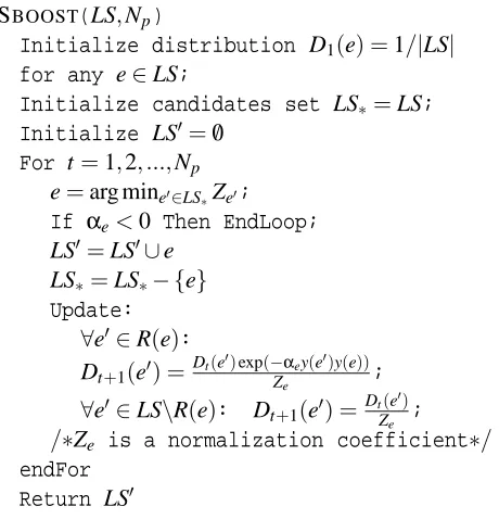
The pseudocode of our algorithm PSBOOSTis described in Figure 2. Note that, in this section,

the confidenceαeis only used for selecting the prototypes and not for generating a weighted

PSBOOST(LS,Np)

Initialize distribution D1(e) =1/|LS| for any e∈LS;

Initialize candidates set LS_∗=LS; Initialize LS0=/0

For t=1,2,...,Np e=arg mine0∈LS∗Ze0;

If α_e<0 Then EndLoop; LS0=LS0∪e

LS_∗=LS_∗− {e} Update:

∀e0∈R(e): Dt+1(e0) =Dt(e

0_)exp(−α

ey(e0)y(e))

Ze ;

∀e0∈LS\R(e): Dt+1(e0) =Dt(e

0₎

Ze ;

/∗Ze is a normalization coefficient∗/

endFor Return LS0

Figure 2: Pseudocode for PSBOOST. The output of this algorithm is the prototype subset LS0.

k-NN CF PSRCG PSBOOST MC RT3 PSBOOST∗

DataSets Acc. Acc. % prot Acc. % prot Acc. Acc. Acc. % prot Acc.

AUDIOLOGY 73.40 73.80 69.8 73.70 86.1 73.84 72.21 69.40 10.7 70.00 AUSTRAL 80.55 79.55 84.2 78.41 58.5 80.27 75.41 70.67 10.9 71.68 BIGPOLE 59.94 60.23 69.8 59.92 88.1 58.91 59.94 58.89 17.5 57.29 BREAST 96.89 96.76 97.5 97.04 10.0 96.19 97.04 87.72 1.2 81.24 BRIGHTON 95.80 94.59 97.6 94.6 32.4 94.46 93.60 90.56 16.4 90.27 BUPA 62.67 65.31 73.0 66.76 79.0 68.77 65.90 63.35 10.8 62.45 ECHOCARDIO 60.00 69.18 68.0 62.58 60.3 61.87 62.63 58.30 5.8 61.87 GERMAN 72.85 72.05 77.8 70.87 73.7 72.65 69.88 69.87 10.6 72.65 GLASS2 72.65 73.31 81.5 72.10 72.7 74.49 70.88 55.07 11.7 60.29 HARD 47.12 45.36 63.4 44.91 90.9 47.85 46.32 48.27 13.4 50.55 HEART 74.21 73.15 81.0 74.56 52.1 79.92 73.13 74.91 6.9 72.72 HEPATITIS 81.73 82.38 88.6 81.20 46.6 76.63 77.95 68.25 9.6 76.56 HORSE 68.98 68.43 79.6 69.48 74.1 72.95 71.87 70.30 9.5 67.89 IONOSPHERE 75.75 74.12 86.4 71.46 65.0 76.73 74.61 74.06 8.4 76.20 LED+17 72.76 75.64 82.3 69.93 81.2 76.12 68.95 64.62 19.8 70.43 LED 89.79 89.20 91.3 87.63 36.9 89.20 86.83 66.79 4.4 74.68 PIMA 67.44 67.82 76.1 66.79 68.2 67.18 64.87 62.65 6.7 65.87 VEHICLE 70.99 70.30 78.8 70.17 69.2 69.95 68.70 58.82 7.8 68.51 WHITEHOUSE 90.76 89.91 93.7 91.47 30.0 90.57 92.60 81.52 4.5 90.11 XD6 80.60 80.46 85.5 80.29 72.0 80.63 80.00 72.26 14.6 74.70 AVERAGE 74.75 75.08 81.3 74.19 62.4 75.46 73.70 68.31 8.7 70.80

Table 1: Results (accuracy Acc. and percentage of selected instances % prot) for kNN (k=5), CF, PSRCG, PSboost, MC (Monte-Carlo), RT3, PSboost∗; PSboost (resp. PSboost∗) means that PSboost is run with exactly the same number of prototypes than PSRCG(resp. RT3)

original goal is to select the most relevant instances from LS. Once the selection is done, the output

method, we compare the performances of LS and LS0 without any other optimization strategy (for instance by generating a weighted classifier).

Some useful observations can be made about the value of Ze and its contribution to removing

irrelevant instances in LS. First, if an instance e belongs to a region with very few instances, it will

not belong to many reciprocal neighborhoods, resulting in a large W0

e, preventing the achievement

of small Ze. Secondly, if a prototype belongs to a region with evenly distributed instances, We+and W_e− tend to be balanced, and this again, prevents to obtain small Ze. Note that with our strategy,

a cluster of instances of the same class could be all picked for LS0, resulting in a redundancy in the final subset. A way to solve this drawback would consist in applying a post-process to remove redundancy. For example, Sebban and Nock (2000) proposed, in another context, to compute an

information measure from a (k+1)-NN graph. Only instances at the center of clusters keep a

null uncertainty with k+1 neighbors. Removing such instances allows the deletion of the useless

instances from the clusters.

Note in Figure 2 that the user must provide a value for Np, the number of prototypes. In this

paper, we provide a theoretical framework for automatically determining Npusing a statistical test.

Nock and Sebban (2001a) carried out a large comparative study between PSBOOSTand the

state-of-the-art prototype selection algorithms for which we recall the main results (obtained by

cross-validation) in Table 1. CF corresponds to the Consensus Filter (Brodley and Friedl, 1996), PSRCG

was proposed by Sebban and Nock (2000), RT3 by Wilson and Martinez (2000), and MC corre-sponds to Monte-Carlo sampling as proposed by Skalak (1994) (for more details see Nock and Sebban (2001a)). Although these results are interesting, the parameter Npmust be fixed in advance,

and that constitutes a drawback for PSBOOSTin its original version.

3. Theoretical Stopping Criterion

In this section, we describe our statistical criterion for automatically halting the selection procedure.

3.1 A Random Framework for Test Construction

In this section, we propose a theoretical framework for determining the number of weak hypotheses

Np. Our strategy is based on a statistical test. Let H0 be the null hypothesis of this test, which

expresses the idea that a given e does not statistically contribute to give information about the

labelling of its reciprocal neighborhood. Informally, as long as H0 can be kept, such an instance

can be removed without reasonably endangering further classification tasks. This requires a statistic that assesses for a given candidate e the validity of H0, and for which we provide the statistical law

under H0. For a given riskθ, we stop the selection if and only if all the candidates have a p-value

higher than θ. Stated differently, the algorithm stops if the best current candidate does not allow the rejection of H0 with a risk smaller thanθ. We provide here a theoretical framework for binary

problems. The extension to multiclass problems is discussed in Section 7.

A possible way of proceeding consists in considering under H0that, in the reciprocal

neighbor-hood R(e), the true class Y is randomly distributed with a given probabilityπ0(if y(e) =1) or 1−π0

(if y(e) =−1). Two ways are possible to fixπ0:

2. Useπ0=0.5 to satisfy a majority vote rule for a 2-class problem, often used in classification

tasks. Stated differently, we test if e classifies instances in R(e)better than a simple coin toss.

Let H0(π0)be the corresponding null hypothesis. Under H0(π0), an instance of the reciprocal neighborhood R(e)belongs to the same class as e with probabilityπ0(resp. 1−π0) if y(e) =1 (resp. y(e) =−1).

3.2 Law of W_e+under H0

In our approach, an instance e is selected by minimizing the quantity Ze,while ensuring a positive

confidenceαe(which avoids the selection of mislabeled instances).

Ze = 2 r

(We++

1

2W

0

e)(We−+

1 2W 0 e) = 2 r

(We++

1

2W

0

e)(1−We+−

1

2W

0

e),

because W_e++W_e−+W_e0=1. Then, Zedepends on the value of We+in R(e):

W_e+ =

∑

e0∈R(e):y(e0)=y(e) Dt(e0)

=

∑

e0∈R(e)

Dt(e0)I_{y(e0)=y(e)},

where the boolean variable I_{y(e0)=y(e)} is 1 iff y(e0) =y(e), and 0 otherwise. If H0(π0) is true, I_{y(e0)=y(e)} follows a binomial law B(1,p), where p=π0if Y(e) =1 else p=1−π0. Considering

that W_e+ depends on examples i,i=1,2,..,|R(e)| (the size of the reciprocal neighborhood), we propose the following simplification:

W_e+ = |R(e)|

∑

i=1

Dt(i)Ii.

There are two different ways to construct the distribution of W_e+ under H0to compute the critical

value of W_e+, called W₁+_−θ. We recall here that the critical value defines the bound of the rejection region of H0, and corresponds to the(1−θ)-percentile of the distribution of We+ under H0. In the

two following approaches, we assume that the Dt(i) are not random variables, even if in theory,

they depend on the labels of the examples. First, the distribution can be assessed by a normal

approximation. In this case, under H0(π0),W_e+ is a weighted sum of|R(e)|variables Ii, where the Iiare independently and identically distributed. The mean and variance of We+are:

E(W_e+/H0) = |R(e)|

∑

i=1

Dt(i)E(Ii)

= p

|R(e)|

∑

i=1 Dt(i)

Var(W_e+/H0) = |R(e)|

∑

i=1

D_t2(i)Var(Ii)

= p(1−p) |R(e)|

∑

i=1

The other way to proceed would consist of simulating the distribution of W_e+, which can deal with

cases where the approximation constraints are not satisfied. For balanced weights (when W_e+ and

W_e−are close),|R(e)|>10 is enough to satisfy these constraints. In an unbalanced case, W_e+must be larger.

3.3 Statistical Test

Without a criterion for halting the selection, PSBOOST requires the provision of the number Np

of weak hypotheses. Such a strategy may lead to the selection of an instance for which the null hypothesis H0would not be rejected. By introducing a statistical test using the critical value W1+−θ, we keep only instances e for which We+is exceptionally high under H0 (i.e., We+>W1+−θ). Among these, we choose at a given stage of the selection the one that minimizes Z, or equivalently Z2. The procedure is stopped if for all the instances e,W_e+<W₁+_−θ.

3.3.1 ASSESSING THECRITICALVALUE OFW_e+

We assess W₁+_−θeither by normal approximation or by simulation, which is computationally

expen-sive, but sometimes necessary if the approximation conditions are not satisfied. By approximation,

W₁+_−θ is easily defined as follows:

W₁+_−θ = p |R(e)|

∑

i=1

Dt(i) +u1−θ

v u u

t_p(1−p)|R

_∑

D2t(i),

where u1−θis the (1−θ)-percentile of the normal law N(0,1). If the approximation constraints are

not satisfied, we can artificially construct a distribution of W_e+, by simulating |R(e)|independent observations Ii according to B(1,p), and computing the weighted sum∑|

R(e)|

i=1 Dt(i)Ii. By repeating

this procedure N times, an estimate of W+

1−θis the (1−θ)-percentile of the N samples.

3.3.2 DECISIONRULE

An instance e is selected by minimizing Ze:

Ze = 2 r

(We++

1

2W

0

e)(We−+

1

2W

0

e),

while ensuring a positive confidenceαe:

αe =

1 2log

W_e++1₂W_e0 We−+1₂We0

!

.

At each stage of the selection, our procedure minimizes the quantity Z2=4F(1−F), where F=

W_e++1₂W_e0. The critical value of F with the riskθis directly deduced from W₁+_−θ:

F1−θ = W1+−θ+

1

2W

0

e

= p

|R(e)|

∑

i=1

Dt(i) +

1

2W

0

e +u1−θ v u u

t_p(1−p)|R

_∑

Under H0(π0), F1−θ can in theory be smaller than 0.5 when p<0.5. In this case, if two candidates satisfy the first condition (W_e+>W₁+_−θ), their confidences are then negative, and paradoxically we will choose the candidate e which presents the smaller value Fe(Fe∈[F1−θ,0.5]), by minimizing Ze. This situation, possible when p is very close to 0,in fact rarely occurs because there is almost always a candidate e0 for which F1−θ>0.5 and Fe0 >F1−θ(Fe0 ∈[F1−θ,1]), often resulting in Ze0 <Ze. This

fact has been confirmed by an experimental study. Actually, on 18 datasets, using a 5-fold cross-validation resulting in 90 different databases, we noted that this situation never occurred. However, the neighborhood-based classifiers, such as the k-nearest-neighbors, usually use a majority decision rule with a threshold 0.5 (in the case of 2 classes). In such a context, it is more suitable to test the null hypothesis H0(0.5), which means that we select only the instance e that classifies, in the reciprocal neighborhood R(e), significantly better than a simple toss. In this case, F>1−F, and

then α>0. Under H0(0.5), we have always p=0.5, and the previous formulae for F_1−θ can be simplified:

F1−θ = 1 2

|R(e)|

∑

i=1

Dt(i) +We0 !

+1

2u1−θ v u u t|R

_∑

i=1 D2t(i)

= 1

2+

1 2u1−θ

v u u t|R

_∑

i=1

D_t2(i).

We deduce the critical values of Z2andαwith the riskθ, called cθandα1−θ: cθ = (2pF1−θ(1−F1−θ))2

= 1−u2_1−θ |R(e)|

∑

i=1 D_t2(i)

α1−θ = 1 2log

F1−θ 1−F1−θ

= 1

2log

1+u1−θ

s

|R(e)| ∑ i=1

D2t(i)

1−u1−θ

s

|R(e)| ∑ i=1

D2

t(i)

.

Then, we select the instance e if and only if Z2_e <c_θ orαe>α1−θ. Note that, while we select the

instance e for which Ze is minimum, we use in the decision rule the law of Ze and not the one of

mineZe. According to the level of dependence of Ze0s, the risk is in fact contained betweenθand

(θ.|LS|). A simulation procedure would allow us to have more information about this problem.

Then, note thatθis more a control parameter than the probability of type 1 error. The new version of our algorithm, called PSBOOST2, is described in Figure 3.

4. The Relative Neighborhood Graph

While PSBOOST2 was originally proposed for improving the k-NN algorithm, our theoretical

frame-work is independent of the geometrical structure used for the construction of the reciprocal

PSBOOST2(LS)

Initialize D1(e) =1/|LS| for any e∈LS; Initialize candidates set LS_∗=LS; Initialize LS0=/0

Repeat

Temp={e0∈LS_∗: W_e+>W₁+_−θ} e=arg mine0∈TempZe0;

If α_e>α_1−θ Then Stop ← False LS0=LS0∪e LS_∗=LS_∗− {e} Update:

∀e0∈R(e): Dt+1(e0) =Dt(e

0_)e−αey(e0)y(e) Ze ;

∀e0∈LS\R(e): Dt+1(e0) =Dt(e

0₎

Ze ;

Else Stop ← True endIf

Until Stop=True Return LS0

Figure 3:Pseudocode for PSBOOST2.

Graph (RNG). Introduced by Toussaint (1980), the RNG is a connected graph in which, if two instances are linked by an edge, then they satisfy the following property:

d(a,b) ≤ min

c∈LS,c6=a,bmax(d(a,c),d(b,c)).

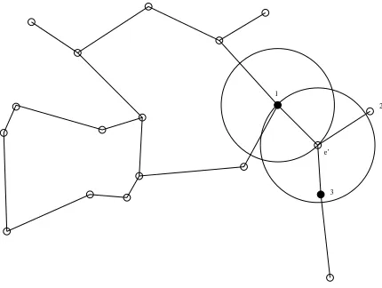
This definition means that La,b, which corresponds to the intersection of two hyperspheres, with

centers a and b and with radius equal to the distance between a and b, does not contain any other point of the learning set LS (Figure 4 describes an example). The RNG can naturally be used in a neighborhood-based classifier. We present here a general framework for problems with an arbitrary number of classes and an arbitrary geometrical structure used for building the neighborhood graph.

Definition 3 Let Ci be the set of learning instances belonging to the i-th class: ∀i = 1,..,c, Ci= {e∈LS : y(e) =i}where c is the number of classes.

Definition 4 Let O(e0)be the c-dimension vector whose components are noted Oi(e0), i = 1,..,c, each being the proportion of instances in the neighborhood of e0belonging to the i-th class:

Oi(e0) = |

N(e0)∩Ci|

|N(e0)| ,∀i=1,2,..,c,

where N(e0)is the set of neighbors of e0(linked by an edge to e0) in the neighborhood graph.

Definition 5 Letφ(e0)be the class given to e0by the classifierφfrom the neighborhood graph (RNG or k-NN):

φ(e0) = arg max

i Oi(e

0_).

According to these definitions, the new instance e0 in Figure 4 would be labeled “black” from its

neighbors 1, 2 and 3.

e’ 1

2

3

Figure 4: Relative Neighborhood Graph: the intersection of the two hyperspheres does not contain any instance of the learning set.

5. Experimental Results

In this section, we assess the efficiency of PSBOOST2 according to the two following performance

measures: generalization accuracy and storage reduction. We used 18 datasets, most of which come from the UCI database repository (Merz and Murphy, 1996). The experimental method was

the following: a f -fold cross-validation (here f =5) was performed on each database to obtain

estimates of the true performance of the classifier. We used two neighborhood-based classifiers

according to the geometrical structures listed above (k-NN, here k=3, and the RNG). The decision

rule used for classifying an instance consists of a majority vote of the neighbors. Each database

DB is divided into f disjoint sets DBi. PSBOOST2 is applied on each combination DB−DBi. The

classifier uses the resulting subset of instances(DB−DBi)subset for classifying the instances in DBi.

For each classifier, we obtain an accuracy estimate by averaging results over the f sets.

Note that we did not conduct a large comparative study between PSBOOST2 and the

state-of-the-art prototype selection algorithms because it was already carried out for PSBOOSTby Nock and

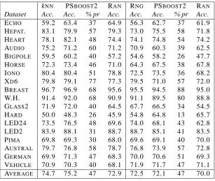
Sebban (2001a), of which the main results are described in Table 1. These results have shown the difficulties that the standard prototype selection algorithms have in controlling the two performance measures. From the results described in Table 2, we can make the following remarks:

kNN PSBOOST2 RAN RNG PSBOOST2 RAN Dataset Acc. Acc. % pr Acc. Acc. Acc. % pr Acc.

ECHO 59.2 63.4 37 64.9 56.3 62.7 37 61.9

HEPAT. 83.1 79.9 57 79.3 73.0 75.5 58 71.8 HEART 78.1 82.1 48 74.4 74.1 74.8 54 74.2 AUDIO 75.2 71.2 60 71.2 70.9 60.3 39 62.5 BIGPOLE 59.5 60.2 40 57.2 54.6 58.2 26 47.7 HORSE 72.3 73.4 46 71.0 64.3 67.5 38 67.8

IONO 80.4 80.4 51 78.8 72.5 73.5 36 68.2

XD6 79.8 79.1 77 77.3 79.5 71.0 57 72.0

BREAST 96.7 96.9 68 95.6 95.5 94.5 88 95.0

W.H. 91.4 92.0 68 90.9 91.1 89.5 80 88.8

GLASS2 71.9 72.0 40 64.5 67.7 66.5 34 54.5

HARD 50.0 48.3 26 45.9 54.8 64.8 13 65.7

LED24 73.5 76.5 48 69.6 74.0 68.1 43 62.8

LED2 83.9 88.1 31 88.7 88.7 85.1 41 83.5

PIMA 69.8 69.3 30 68.0 69.6 69.1 40 70.0

AUSTRAL 79.7 76.8 58 78.7 76.8 73.9 57 72.8 GERMAN 69.9 71.3 47 68.3 70.0 70.6 51 69.3 VEHICLE 70.9 70.3 40 68.1 71.9 71.7 47 71.1 AVERAGE 74.7 75.2 47 72.9 72.5 72.1 47 70.0

Table 2: Effect of PSBOOST2 on learning set size and generalization accuracy on 18 datasets; k-NN, RNG correspond respectively to the accuracy on DBi, using the whole learning set, with a 3-NN classifier and a voting rule based on the RNG; PSBOOST2 is described by its accuracy (Acc.) and its storage requirement (% pr); RANcorresponds to the accuracy achieved from a learning subset of same size (LS0) randomly selected in|LS|.

over accuracies, the predictive accuracy of the post-PSBOOST2 nearest neighbor classifier is increased (74.7% vs. 75.2%), even though this superiority is not significant with a p-value

near 0.5. Therefore, it seems to confirm experimentally that PSBOOST2 is suited to control

the generalization accuracy while significantly reducing the data.

2. A simple strategy for assessing the relevance of PSBOOST2 consists in comparing the

se-lected subset (LS1) with another one (LS2) of the same size but randomly selected from LS.

Such a procedure allows one to estimate the quality of the selected prototypes. We made this comparison (columns PSBoost2/Acc. and Ran in Table 2). Our strategy achieves a signif-icantly higher accuracy than a random one, and this also tends to confirm the efficiency of PSBOOST2.

6. Some Insights into the Performances of PSBOOST2

In this section, we explain why PSBOOST2 is suited for reducing storage while controlling the

6.1 PSBOOST2 and Margin Maximization

A partial explanation of PSBOOST2’s performances may rely on the margin maximization principle.

This principle is in fact not recent, and was originally suggested in Vapnik (1982) for support vector machines (SVMs) with optimal margins. Even though the objective in both approaches consists in finding classifiers which maximize margins on learning data, a detailed study of their mechanisms shows that they slightly differ (Schapire et al., 1998). In SVMs the sum of squared outputs of the

base hypotheses and the sum of the squared weights are both assumed to be bounded (l2 norm),

while in boosting the maximum value of the base hypotheses (l_∞norm) and the sum of the absolute

values of the weights (l1 norm) are assumed to be bounded. Support vector machines give rise to

a quadratic programming problem, whereas the optimization in boosting can be seen as a linear programming problem.

In Schapire et al. (1998), the authors prove that achieving a large margin on LS results in an

improved bound on the generalization. They also prove that ADABOOST is suited to maximizing

the number of learning examples with large margin. They define classification margin as the dif-ference between the weight assigned to the correct label and the maximal weight assigned to any single incorrect label. The margin is then a number in the range [-1,+1] and an example is correctly classified if it has a positive margin. The margin also corresponds to a degree of confidence in the

classification. In order to assess the effect of PSBOOST2 for maximizing margins, we computed

for the k-NN classifier the margin gain gi for each dataset i over the 5 folds (before and after

PS-BOOST2). We first observe that over the 18 datasets, the average margin gain G=₁₈1 ∑gi=0.24.

This might be an experimental explanation for the accuracy’s control in PSBOOST2. Even more,

a second observation displays the ability of PSBOOST2 to increase margins, as all datasets have a

margin gain gi>0.

6.2 The Filter Precision of PSBOOST2

Brodley and Friedl (1996) provided a method for evaluating the ability of a data reduction technique to identify and eliminate mislabeled instances (called filter precision). This procedure in a way assesses the sensitivity to noise. Consider a learning set artificially corrupted by a given percentage of noise. One defines the 3 following sets: the set D of instances discarded, the set M of instances

a priori corrupted, the set M∩D of corrupted instances discarded by the data reduction technique.

Brodley and Friedl defined P(E)as an estimate of the probability of retaining bad data:

P(E) = |M| − |M∩D|

|M| .

While the original 18 datasets probably already contain noisy data, we decided to calculate P(E)

for different artificial noise levels. We corrupted the original data successively with 5, 10, ..., 35%

noise. Table 3 reports P(E) averaged over all datasets and all folds for the k-NN and the RNG

classifiers.

In the presence of noise, the subset of instances (described by its accuracy Acca f t) selected

by PSBOOST2 is always better than the original learning set (Accbe f). The accuracy is actually

improved after prototype selection and this trend seems to speed up with the noise level. This phenomenon is not really surprising. Indeed, noise smoothes class distributions near their frontiers.

NOISE P(E)WITHkNN P(E)WITHRNG Accbe f Acca f t P(E) Accbe f Acca f t P(E)

5% 71.7 72.5 0.07 68.6 68.7 0.15

10% 67.9 69.3 0.08 65.9 66.7 0.15

15% 64.1 67.6 0.07 62.5 63.9 0.17

20% 63.5 66.0 0.08 59.1 60.6 0.16

25% 61.2 64.1 0.08 58.5 59.5 0.17

30% 58.7 61.1 0.08 56.4 58.3 0.19

35% 56.3 60.1 0.09 54.1 56.1 0.18

Table 3:PSBOOST2’s filter precision

7. Extension to Multiclass Problems

In this section, we present the extension of the test to multiclass problems.

7.1 Test on Ze

So far, we have only treated binary problems. Many real-world learning problems are in fact mul-ticlass with many more possible labels. Two main strategies have been proposed to deal with this extension to multiclass problems. The first one consists in creating one binary problem for each of the c classes. Then, we test one class j against all the other classes, answering the following question: “Does the example belong to the jthclass or not?” This approach is called one-against-all (Allwein, Schapire and Singer, 2000). The second one consists in testing all pairs of classes (Hastie and Tibshirani, 1998). For each distinct pair of classes c1,c2, the examples labeled c1 are

consid-ered positive, those labeled c2are negative. All other examples are ignored. This approach is called all-pairs. An interesting comparison is presented in Allwein, Schapire and Singer (2000). In our

approach, we decided to choose the first method (one-against-all) which requires the construction of c binary problems.

In the test proposed for solving binary problems (see Section 3.3), a candidate is selected when

the corresponding Ze=2

p

Fe(1−Fe)is minimum (where Fe = We+ + 12We0), while Fe>F1−θ.

We recall that F1−θis the critical value of Feat the riskθunder H0(π0), the hypothesis that the true

class is randomly attributed with a given probabilityπ0, in the reciprocal neighborhood R(e).

In this section, for multiclass problems, we denote by Fj,e the value of Fe when the class j

is tested against the others. We propose to select the candidate e for which the quantity Ze =

2pFe(1−Fe)is minimum, when Feis defined as follows:

Fe =

1

c c

∑

j=1 Fj,e.

The suspensive condition to select e is the following: Fe>F1−θ, where F1−θ is the critical value

of Fe at the risk θunder the null hypothesis. When the class j is tested against the others, the

null hypothesis, denoted by H0(πj0), means that the class j is randomly distributed with a given

probability πj0 in Rj(e), the reciprocal neighborhood of e when the class j is tested against the

have to define µ andσ2such as:

µ = E(Fe)

= 1

c c

∑

j=1 E(Fj,e)

= 1

c c

∑

j=1

(

∑

e0∈Rj(e)

pjDjt(e0) +

1

2W

0

j,e)

σ2 _{= Var(F}

e)

= 1

c2

c

∑

j=1

Var(Fj,e)

= 1

c2

c

∑

j=1e0∈

∑

pj(1−pj)D2jt(e0),

where Djt(e0)is the distribution at the stage t of the boosting, when the class j is tested against all

the others. We note pj=πj0if Y(e) = j else pj=1−πj0. According to the simplification proposed

in Section 3.2,

µ = 1

c c

∑

j=1 (|

Rj(e)|

∑

i=1

pjDjt(i) +

1

2W

0

j,e)

σ2 ₌ 1 c2

c

∑

j=1 |Rj(e)|

∑

i=1

pj(1−pj)D2jt(i).

We assume in the calculation ofσ2the independence of the Fj,e. Said differently, we consider that

the knowledge of Rj(e), from which Fj,eis computed, does not contain information about the nature

of the reciprocal neighborhood Rl(e), when j6=l. Actually, even if the quantity|Rj(e)|remains the

same∀j, the labels and the weights of the neighbors in Rj(e)will differ according to the tested class j. From this point of view, covariances can be considered as insignificant.

Moreover, note that variables Fj,e are computed from independent variables, then they are not

too far from a normal distribution. Furthermore, as mentioned before, they are approximately

inde-pendent. Then, we can claim that Fe is very close to a normal distribution. We can determine the

critical values F1−θand cθfor Feand Ze2:

F1−θ = µ+u1−θσ

cθ = 4F1−θ(1−F1−θ).

Note that for the special case where pj=0.5 (for satisfying an absolute decision rule), the previous

formulae are highly simplified. Actually,

|Rj(e)|

∑

i=1

pjDjt(i) +

1

2W

0

j,e =

1 2(W

+

j,e+Wj−,e) +

1

2W

0

j,e

= 1

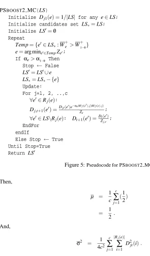
PSBOOST2 MC(LS)

Initialize Dj1(e) =1/|LS| for any e∈LS;

Initialize candidates set LS_∗=LS; Initialize LS0=/0

Repeat

Temp={e0∈LS_∗: W+_e >W+_1−θ} e=arg mine0∈TempZe0;

If α_e>α_1−θ Then Stop ← False LS0=LS0∪e LS_∗=LS_∗− {e} Update:

For j=1, 2, ..,c

∀e0∈Rj(e): Dj,t+1(e0) =

Djt(e0)e−αeM(y(e0),j)M(y(e),j)

Ze ;

∀e0∈LS\Rj(e): Dt+1(e0) =Dt(e

0₎

Zj,e ;

EndFor endIf

Else Stop ← True Until Stop=True Return LS0

Figure 5: Pseudocode for PSBOOST2 MC.

Then,

µ = 1

c c

∑

j=1 (1

2)

= 1

2 .

And,

σ2 ₌ 1

4c2

c

∑

j=1 |Rj(e)|

∑

i=1

D2_jt(i).

The pseudocode of our extended algorithm, called PSBOOST2 MC, is described in Figure 5. Note

that we use in this algorithm the coding matrix M(y(e),j)which was originally given by Dietterich

and Bakiri (1995). For the one-against-all approach, M is a c×c matrix in which all diagonal

elements are positive (+1) and all other elements are negative (−1). When a class j is tested against the others, the current label of the instance e is the value M(y(e),j), where y(e)∈ {1,2,..,c}.

7.2 Experimental Results

DATASET #CLASSES |LS| #FEATURES

WAVES 3 500 21

ABALONE 3 1000 8

GLASS 6 214 9

BALANCE 3 625 4

IRIS 3 150 4

LED 10 500 7

LED+17 10 500 24

DERMATOLOGY 6 366 34

Table 4:Multiclass classification problems.

1 2 3 4 5 6 7 8 9 10 72

70

68 71

69

k Accuracy

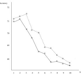
Figure 6: Contribution of PSBOOST2 MC on multiclass problems: the solid line corresponds to the accu-racy of a standard k-NN classifier, built from the whole learning sample; the dashed-line represents the success rate computed from the reduced learning set.

used many values of k (k=1,2,..,10) in the k-nearest neighbor classifier. Except for this detail, the experimental method remains the same as the previous study, namely the 5-fold cross-validation. A graphic synthesis of the results is presented on Figure 6. Each point of this figure is the average over the eight datasets, each of them tested five times during the cross-validation. Therefore, one point corresponds to the average of forty accuracies. Beyond data reduction, the results display

the positive contribution of PSBOOST2 MC to the accuracy’s increase: for all values of k, the

8. Weighted Classifiers using Instance Confidences

Beyond prototype selection, this section aims at exploring an issue that was raised by Sebban, Nock and Lallich (2001): the use of boosting-derived weights for weighted nearest neighbor rules. In such a context, the classification rule (as defined in Section 4) must be slightly modified, since the classification rule does not handle classes anymore, but real weights in favor of each class. The following definition for O(e0)replaces Definition 4:

Definition 6 Let O(e0)be the c-dimension vector whose components are noted Oi(e0), i=1,2,..,c, each being the sum of weights of the instances in the neighborhood of e0belonging to the i-th class:

Oi(e0) =

∑

αe,∀i=1,2,..,c.

Note thatαeis still the confidence of the instance e when e is selected, but we end up selecting all

instances. The weighting algorithm is a slight variant of PSBOOST2 MC, in which the condition

W_e+>W_e−is removed. This little algorithmic difference is crucial, as some instances may now have a negative weight. This still makes sense, because the new rule leverages the neighborhood vote in favor of some classes, or in disfavor of others when negative weights abound.

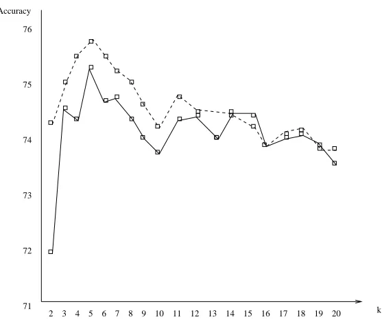
Experimental studies have been conducted with a k-nearest neighbor classifier, for k=1,2,..,20. We applied our approach on twenty-three datasets. Rather than presenting the twenty-three curves (one for each dataset), we synthesize the results in one figure, where each point is the average of

5 (folds) ×23 (datasets) = 115 accuracies. Results are presented in Figure 7. It appears that the

performance of the standard k-NN rule is almost systematically improved by leveraging votes with the boosting weights. Even more, a Student paired t-test reveals that the difference between the standard k-NN and our weighted k-NN is significant for all values k=1,2,..,11. For k large enough

(k≥12), the difference becomes insignificant. This can be explained by the fact that large values

of k tend to smooth neighborhood distributions (ultimately, they become the whole sample’s), for which weighting brings no significant difference.

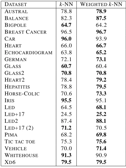
Another concise way to display the results consists in putting separately the results for each dataset, as an average over the different values of k. Instead of identifying the good values of k, we identify the good datasets, candidate for an improvement with our weighted nearest neighbor

rule. We choose to take into account only the values of k<12, for which weighting brings on

average a statistical advantage. The results are presented in Table 5 and graphically represented in Figure 8. We can note that for 17 datasets, a weighted decision rule provides better results than the unweighted rule. Among them, 7 datasets (Balance, Echocardiogram, German, Horse Colic, Led,

Pima and Vehicle) see important improvements, ranging from 1% to>5%. In contrast, only one dataset sees significant accuracy decrease (Car, 96.0% vs. 93.9%).

9. Conclusions and Future Research

76

75

74

73

72

71

2 3 4 5 6 7 8 9 10 11 12 13 14 15 16 17 18 19 20 Accuracy

k

Figure 7: Comparison between a standard k-NN classifier (solid line) and a weighted classifier using the relevance of each instance (dashed-line).

interesting direction of research consists in finding such a method tailored to processing data for induction algorithms, such as, for example, decision tree induction.

Furthermore, we have shown that instead of reducing the learning set size, the boosting-derived weights can be experimentally used in weighted nearest neighbor rules, with statistical advantage compared to the usual, unweighted rules. Because it boils down to making boosting with instances as weak learners that abstain, and because nearest neighbor rules are among the earliest, simplest and still widely used classifiers, this algorithm certainly deserves theoretical investigations to cast, among all, the boosting theory and results (Freund and Schapire, 1997; Schapire and Singer, 1998).

Acknowledgements

The authors wish to thank the referees and Colin de la Higuera for many useful remarks. Our warmest thanks go to Xiaoli Zhang and Carla Brodley, whose invaluable and numerous comments were the basis of a significant improvement of the paper.

References

Erin Allwein, Robert E. Schapire and Yoram Singer. Reducing multiclass to binary: a unifying approach for margin classifiers. Journal of Machine Learning Research, 1, 113–141, 2000.

Leo Breiman, Jerome H. Friedman, Richard A. Olshen and C.J. Stone. Classification And

DATASET k-NN WEIGHTEDk-NN

AUSTRAL 78.8 78.9

BALANCE 82.3 87.5

BIGPOLE 64.7 64.2

BREASTCANCER 96.5 96.7

CAR 96.0 93.9

HEART 66.0 66.7

ECHOCARDIOGRAM 63.8 65.2

GERMAN 72.1 73.1

GLASS 60.7 60.4

GLASS2 70.8 70.8

HEART2 78.4 79.2

HEPATITIS 78.8 79.5

HORSE-COLIC 70.6 73.3

IRIS 95.5 95.1

LED 64.5 68.1

LED+17 24.5 25.2

LED2 87.4 88.1

LED+17 (2) 71.2 70.5

PIMA 68.2 69.8

TIC TAC TOE 75.3 75.6

VEHICLE 70.0 71.4

WHITEHOUSE 91.3 90.9

XD6 79.5 79.5

Table 5: Average accuracy computed over twenty-three datasets by a standard k-NN and a weighted k-NN, where k=1,2,..,11; an accuracy in bold font means that this accuracy is the best value.

Carla Brodley and Mark A. Friedl. Identifying and eliminating mislabeled learning instances. In Proceedings of the Thirteen National Conference on Artificial Intelligence, pages 799–805, AAAI Press, 1996.

Thomas M. Cover and Peter E. Hart. Nearest neighbor pattern classification. IEEE Transactions on

Information Theory, 13, 21–27, 1967.

Thomas G. Dietterich and Ghulum Bakiri. Solving multiclass learning problems via error-correcting output codes. Journal of Artificial Intelligence Research, 2, 263–286, 1995.

Yoav Freund and Robert E. Schapire. Experiments with a new boosting algorithm. In

Proceed-ings of the Thirteenth International Conference on Machine Learning, pages 148–156, Morgan

Kaufmann, 1996.

Yoav Freund and Robert E. Schapire. A decision theoretic generalization of online learning and an application to boosting. International Journal of Computer and System Sciences, 55(1), 119-139, 1997.

Geoffrey W. Gates. The reduced nearest neighbor rule. IEEE Transactions on Information Theory, 18, 431–433, 1972.

50 60 70 80 90 100 100

90

80

70

60

50

Breast

Glass

Glass2

Austral Heart

Hepatitis

Horse

Led+17(2) German

Tic tac toe Vehicle

Led Pima

Bigpole Heart2 Echocardio

Iris Car

Led2

Balance White House

Xd6

Accuracy with a standard kNN

Accuracy with a weighted kNN

Figure 8: Scatterplot (standard k-NN classifier vs. weighted k-NN classifier) on twenty-three datasets. Each dot under the y=x line depicts a dataset for which the weighted k-NN is not better than the

standard k-NN.

Trevor Hastie and Robert Tibshirani. Classification by pairwise coupling, The Annals of Statistics, 26(2), 451–471, 1998.

George H. John, Ron Kohavi and Karl Pfleger. Irrelevant features and the subset selection problem. In Proceedings of the Eleventh International Conference on Machine Learning, pages 121–129, Morgan Kaufmann, 1994.

Daphne Koller and Mehran Sahami. Toward optimal feature selection. In Proceedings of the

Thir-teenth International Conference on Machine Learning, pages 284–292, Morgan Kaufmann, 1996.

Christopher J. Merz and Philip M. Murphy. UCI repository of machine learning databases,

HTTP://WWW.ICS.UCI.EDU/MLEARN/MLREPOSITORY.HTML, 1996.

Richard Nock and Marc Sebban. Advances in adaptive prototype weighting and selection.

Interna-tional Journal on Artificial Intelligence Tools, 10 (1-2), 137–156, 2001a.

Richard Nock and Marc Sebban. An improved bound on the Finite Sample Risk of the Nearest Neighbor Rule. Pattern Recognition Letters, 22, 413-419, 2001b.

Richard Nock and Marc Sebban. Sharper bounds for the hardness of prototype and feature selection. In Proceedings of the International Conference on Algorithmic Learning Theory, pages 224–237, Springer Verlag, 2000.

Robert E. Schapire, Yoav Freund, Peter L. Bartlett and Wee Sun Lee. Boosting the margin: a new explanation for the effectiveness of voting methods.Annals of Statistics, 26, 1651–1686, 1998. Marc Sebban. On feature selection: a new filter model. In Proceedings of the Twelfth International

Florida Artificial Intelligence Research Society Conference, pages 230–234, AAAI Press, 1999.

Marc Sebban and Richard Nock. Instance pruning as an information preserving problem. In

Pro-ceedings of the Seventeenth International Conference on Machine Learning, pages 855–862,

Morgan Kaufmann, 2000.

Marc Sebban, Richard Nock, and Stephane Lallich. Boosting Neighborhood-Based Classifiers. In

Proceedings of the Eighteenth International Conference on Machine Learning, pages 505–512,

Morgan Kaufmann, 2001.

David Skalak. Prototype and feature selection by sampling and random mutation hill climbing algorithms. In Proceedings of the Eleventh International Conference on Machine Learning, pages 293–301, Morgan Kaufmann, 1994.

Godfried Toussaint. The relative neighborhood graph of a finite planar set. Pattern Recognition, 12, 261–268, 1980.

Vladimir N. Vapnik. Estimation of dependences based on empirical data. Springer-Verlag, 1982. Randall Wilson and Tony R. Martinez. Improved heterogeneous distance functions. Journal of

Artificial Intelligence Research, 6, 1–34, 1997.