DBM-Tree: A Dynamic Metric Access Method Sensitive to
Local Density Data
Marcos R. Vieira, Caetano Traina Jr., Fabio J. T. Chino, Agma J. M. Traina
Department of Computer Science, University of S˜ao Paulo at S˜ao Carlos, S˜ao Carlos, SP - Brazil {mrvieira,caetano,chino,agma}@icmc.usp.br
Abstract. Metric Access Methods (MAM) are widely employed to speed up the evaluation of similarity queries, such as range andk-nearest neighbor queries. Most of the currently MAM available today achieve reasonable good performance of query evaluation through minimizing the number of disk accesses required to evaluate a query. The classical way of minimizing the number of disk accesses in hierarchical access methods is to keep the height of the structures very short. This class of structures is called height-balanced structures and are widely employed in Database Management Systems (DBMS). Slim-tree and M-tree are examples of MAM that are height-balanced structures which achieve very good performance both in terms of disk accesses and running time mainly because the height of the trees are kept very short. However, the performance of these two structures degrade very easy because the covering radius of nodes and the overlapping between nodes increase in a way that a large number of subtrees have to be analyzed when processing a query. This paper presents a new dynamic MAM called the DBM-tree (Density-Based Metric tree), which can minimize the overlap between “high-density” nodes by, in a controlled way, “relaxing” the height-balancing of the structure. Thus, the height of the tree is higher in denser regions in order to keep a tradeoff between breadth-searching and depth-searching. We also present a new optimization algorithm calledShrink, which improves the performance of already built DBM-trees by reorganizing the elements among their nodes. Experiments performed over several synthetic and real-world datasets showed that the DBM-tree is on average 50% faster than traditional MAM. The DBM-tree also reduces the number of distance calculations by up to 72% and disk accesses by up to 54% for answering queries. After performing theShrinkalgorithm, query performance of the DBM-tree improves up to 30% regarding the number of disk accesses. In addition, the DBM-tree scales up well, exhibiting sub-linear performance when increasing the database size.
Categories and Subject Descriptors: Information Systems [Miscellaneous]: Databases
Keywords: indexes, metric access methods, similarity queries
1. INTRODUCTION
In the last decades, the volume of data managed by Database Management Systems (DBMS) is increasing in large proportions. Moreover, new complex data types, such as multimedia data (image, audio, video and long text), geo-referenced information, time series, fingerprints, genomic data and protein sequences, among others, have been incorporated to DBMS. In order to handle these new complex data types and the continuously increasing volume of data managed by DBMS, new index structures, as well as new query processing techniques, have been proposed.
The main technique employed to speed up query processing in commercial DBMS is building effi-cient index structures, also know as Access Methods (AM). Commercial DBMS work pretty well on traditional data domains, e.g. numbers and short strings of characters, because on such domains the total ordering property holds among elements in the data domain. For example, we can establish
A previous version of this paper was published in the XIX Brazilian Symposium on Databases [Vieira et al. 2004]. This work was supported by the FAPESP (S˜ao Paulo State Research Foundation) under grants 01/11987-3, 01/12536-5 and 02/07318-1, and CNPq (Brazilian National Council for Supporting Research) under grants 52.1685/98-6, 52.1267/96-0 and 8652.1267/96-0.52.1267/96-068/52.1267/96-052.1267/96-0-7.
total ordering among natural numbers using the “<” relational operator, e.g. 2 <5 <7 <13. Many AM used by DBMS today, like the B-tree [Bayer and McCreight 1972] and the B+-tree [Comer 1979],
can answer interval and equality queries very efficiently because the total ordering property can be explored. In other words, in each step of the search evaluation a large number of elements can be “pruned” from the search space.
Unfortunately, the total ordering property does not hold for most of the complex data domains [Faloutsos 1996], which makes the use of traditional AM to index and query complex data infeasible. Nevertheless similarity queries are more intuitive in these data domains and comparison is performed between pair of elements. For a given reference element, also calledquery element, a similarity query returns all elements that meet a given similarity criteria w.r.t. the query element. Traditional AM rely on the total order relationship only, and are not able to handle these complex data properly or to answer similarity queries over such data. On the other hand Metric Access Methods (MAM) are well-suited to answer similarity queries over complex data types.
MAM such as Slim-tree [Traina Jr. et al. 2000], [Traina Jr. et al. 2002] and M-tree [Ciaccia et al. 1997] were developed to answer similarity queries based on the similarity relationships among pairs of elements. The similarity relationships are usually represented by distance functions computed over pair of elements. The data domain and distance function defines a metric space. Formally, a metric space is a pair<S, d >, whereS is the data domain anddis a distance function that complies with
the following three properties:
—symmetry: d(s1, s2) = d(s2, s1),s1∈S ands2∈S;
—non-negativity: 0< d(s1, s2)<∞ifs16=s2, andd(s1, s1) = 0; and
—triangle inequality: d(s1, s2)≤d(s1, s3) +d(s3, s2),∀s1, s2, s3∈S.
Vector domains with any Lp distance function, such as Euclidean distance (L2) and Manhattan
distance (L1), are special cases of metric spaces [Chavez et al. 2001], [Hjaltason and Samet 2003]. The
two most common types of similarity queries are:
—Range query - RQ: given a query elementsq ∈S, a maximum query distancerq, and a search
domainS ⊆S, RQ(sq, rq) returns a set of elements R⊆S, such that ∀si ∈R, d(si, sq)≤rq. An
example is: “Select all proteins that are similar to the proteinpby up to 5 purine bases”, and it is represented asRQ(p,5);
—k-Nearest Neighbor query - kN N Q: given a query elementsq ∈Sand an integer valuek≥1,
kN N Q(sq, k) returnsR⊆S containingkelements that have the smallest distance from the query elementsq, according to the distance functiond, that isk=|R|and∀si∈R, sj ∈ {S−R}, d(sq, si)≤
d(sq, sj). An example is: “Select the 3 most similar proteins to proteinp”, and it is represented as
kN N Q(p,3).
This paper presents a new dynamic MAM called DBM-tree (Density-Based Metric tree), which can minimize the overlapping among nodes with elements in high-density regions by relaxing the height of the structure. Thus, the height is higher for subtrees that cover areas with high density of elements in order to keep a “compromise” between the number of disk accesses required to perform a breadth-search in several subtrees and to perform a depth-search in one subtree. We show in our experiments that the query performance of the DBM-tree is better than the “rigidly” balanced trees (Slim-tree and M-tree). In order to further optimize already built DBM-trees we propose an optimization algorithm called Shrink, which reorganizes elements among subtrees in order to reduce even more the overlapping among nodes.
number of distance calculations required to answer similarity queries. After optimizing DBM-trees with theShrinkoptimization algorithm, the total number of disk accesses to answer similarity queries decreased up to 30% compared with non-optimized DBM-trees. We also show in our experiments that the DBM-tree is scalable regarding the database size, exhibiting sub-linear behavior in the total processing time, the number of disk accesses and the number of distance calculations.
The remainder of this paper is organized as follows: Section 2 presents the basic concepts used in this paper; Section 3 summarizes the related work; The DBM-tree organization and algorithms are explained in Section 4; Section 5 describes the experiments performed in order to compare the DBM-tree with the Slim-DBM-tree and M-DBM-tree; and Section 6 concludes the paper and suggests new directions of research.
2. BACKGROUND
Access Methods (AM) are one of the most used resources for improving search performance in DBMS. AM employ important properties of the data domain to achieve good performance. One of the most used properties in hierarchical access methods is the total ordering property. Using this very useful property it is possible to discard large subsets of data even without comparing them with the query element. For example, consider the case of numeric data where the total ordering property holds; this property allows us to split a dataset in this domain into two subsets: a subset with all numeric elements that are greater than a reference numeric element; and a subset with numeric elements that are smaller or equal than a reference numeric element. Hence, one efficient way to perform several searches in a numeric domain is to maintain the dataset in this domain sorted. Then, whenever there is a need to perform a search using a query number on this domain, comparing the query number with a “particular” number in the dataset enables the search algorithm to discard further comparisons with the part of the data where the number cannot be in. A well-know example of a search algorithm that employes this property is the one used in the B+-tree [Comer 1979].
One very important class of AM is the hierarchical structures (or tree structures), which enables recursive processes to index and search the data. These structures can be classified as (height-)balanced or unbalanced, where in the first case the heights of all subtrees in the same level of a tree are the same, or at most they differ by a fixed amount. The elements are stored in blocks called nodes. When a search is performed, the query element is compared with one or more elements in the root node to decide which subtree(s) need to be traversed. This process is repeatedly applied to each subtree that can possibly store elements that belong to the answer set.
Note that whenever the total ordering property applies, only a single subtree at each tree level can hold the answer for equality queries. If the partial ordering property applies to a data domain, then it is possible that more than one subtree need to be analyzed in each tree level. As numeric domains possess the total ordering property, trees indexing numbers require access of only one node at each level of the structure. On the other hand, trees storing spatial coordinates, which only have a partial ordering property, require searches in more than one subtree in each level of the structure. This effect is known as covering of nodes, or overlapping between subtrees, and happens in structures like R-trees [Guttman 1984], [Sellis et al. 1987], [Beckmann et al. 1990].
in commercial DBMS.
Metric Access Methods (MAM), or just metric trees, divide a particular dataset in one or more regions, and choose representative elements for each region to represent them. Each node in a MAM stores a single representativesrep (there are structures that store more than one representative, e.g. MVP-tree [Bozkaya and ¨Ozsoyoglu 1997]), the minimum distance radius srep.radius from the repre-sentative element that covers the entire covering region of the node, a set of elements {s1, s2, ..., sc}
inside its covering regionsrep.radius, and the distance from each element covered in its radius to the representative of the node {d(srep, s1), d(srep, s2), ..., d(srep, sc)}. This node representation is
com-monly used for leaf nodes, and for index nodes the representative elementsihas also a pointer to the subtreesi.subtreethat is covered by the radiussi.radius. Using this general representation, a hierar-chical structure is build to construct a metric tree. Whenever a query is evaluated, the query element is first compared with the representatives of the root node. The triangle inequality is then used to prune subtrees, avoiding distance calculations between the query element and elements or subtrees in the region pruned. Distance calculations between complex elements can have a high computational cost to calculate. Therefore, to a MAM to achieve a good query performance, not only the number of disk accesses has to be minimal, but also the number of distance calculations.
There are two very useful ways to employ the triangle inequality property to avoid calculating distance between elements and the query element. The first one is for pruning the whole subtree
si.subtreeusing the distance between its representative si and the query element sq. If the distance betweensq andsiis greater than the query radiusrq plus the radius of the subtreesi.radius, then we can safely pruneall elements in the subtreesi.subtree. In other words, ifd(sq, si)> rq+si.radius, then there is no element in the whole subtree si.subtreethat qualify to be in the answer set. The second one is avoiding computing the distance calculationd(si, sq), and thus the subtreesi.subtreeas well, between the query elementsq and the representative of a subtree si. If the difference between the distanced(srep, sq) andd(srep, si) is greater than the query radiusrq plus the radius of the subtree
si.radius, then we do not need to compute d(si, sq) to safe prune the whole subtree si.subtree. In other words, if|d(srep, sq)−d(srep, si)|> rq+si.radius, then we do not need to computed(sq, si) to prunesi.subtree.
The effect of node overlapping is observed in all dynamic MAM that are well suitable to work on disk. When a similarity query is performed, the total number of disk accesses depends both on the height of the tree (depth-search) and on the amount of overlapping among the nodes (breadth-search). In this case, it is not worthwhile reducing the number of levels at the expense of increasing the overlapping among nodes. Indeed, reducing the number of subtrees that cannot be pruned at each node may be more important than keep the tree balanced. As more node accesses also requires more distance calculations, increasing the pruning ability of a MAM becomes even more important. To the best of the authors’ knowledge, no one considered this observation so far for dynamic MAM. The DBM-tree is the first dynamic MAM that “breaks” the widely studied and employed paradigm of building height-balancing structures for persistent data on disk. The proposed DBM-tree considers “relaxing” the height-balancing policy in a “controlled” way in order to build unbalanced subtrees in denser regions of the dataset for a reduced overlapping among subtrees. In our experimental evaluation we show that this “break of paradigm” works very well ineverymeasurement observed (disk accesses, distance calculations and running time) for similarity queries using the DBM-tree.
3. RELATED WORK
1999], being efficient only to index low-dimensional datasets (see [B¨ohm et al. 2001]).
Metric Access Methods (MAM) seem to be more attractive for a broad class of applications. Two good surveys on MAM can be found in [Chavez et al. 2001] and [Hjaltason and Samet 2003]. The techniques of recursive partitioning the data in metric domains proposed in [Burkhard and Keller 1973] were the starting point for the development of MAM. The first technique divides the dataset choosing one representative (routing element) for each subset, grouping the remaining elements according to their distances to the representatives. The second technique divides the original set in a fixed number of subsets, selecting one representative for each subset. Each representative and the biggest distance from the representative to all elements in the subset are stored in the structure to improve nearest-neighbor queries. The GH-tree proposed by Uhlmann [Uhlmann 1991] and the VP-tree (Vantage-Point tree) [Yianilos 1993] are examples based on the first technique described in [Burkhard and Keller 1973]. Aiming to reduce the number of distance calculations to answer similarity queries in the VP-tree, Baeza-Yates et al. proposed the FQ-tree [Baeza-Yates et al. 1994] where the same representative is used for every node in the same level. The MVP-tree (Multi-Vantage-Point tree) [Bozkaya and
¨
Ozsoyoglu 1997], [Bozkaya and ¨Ozsoyoglu 1999] is an extension of the VP-tree, allowing selectingM
representatives for each node in the tree. Using many representatives the MVP-tree requires lesser distance calculations to answer similarity queries than the VP-tree. The GH-tree (Generalized Hyper-plane tree) [Uhlmann 1991] is another method that recursively partitions the dataset into two groups, selecting two representatives and associating the remaining elements to the nearest representative. The GNAT (Geometric Near-Neighbor Access tree) [Brin 1995] can be viewed as a refinement of the second technique presented in [Burkhard and Keller 1973], where it stores the distances between pairs of representatives and the biggest distance between each stored element to each representative. The GNAT uses these information and the triangle inequality to prune distance calculations.
Unfortunately all of the MAM discussed so far are static in the sense that the tree is built at once using the whole dataset, and new insertions are not allowed afterward. Furthermore, they mostly attempt to reduce the number of distance calculations, paying no attention on disk accesses. The M-tree [Ciaccia et al. 1997] was the first MAM to overcome these deficiencies. It is a height-balanced tree based on the second technique of [Burkhard and Keller 1973], with data elements stored in leaf nodes. The Slim-Tree [Traina Jr. et al. 2000], [Traina Jr. et al. 2002] is an “evolution” of M-Tree, embodying the first published method to reduce the amount of node overlapping, called the Slim-Down. TheSlim-Downprocess leads to a smaller number of disk accesses to answer similarity queries by reorganizing elements in the leaf level of the tree. Although dynamic, neither the Slim-tree nor the M-tree have element deletion operations described. In [Santos et al. 2001], it is proposed to use multiple representatives, called “omni-foci”, to generate a coordinate system for the dataset. The coordinates can be indexed using any SAM, ISAM (Indexed Sequential Access Method), or even sequential scanning, generating a family of MAM called the “Omni-family”.
The dynamic MAM described so far build balanced trees. The main reason of building height-balanced trees is to minimize the tree height at the expense of little flexibility in reducing overlap among nodes. Overlapping nodes degenerates query performance mainly because all nodes that has some overlap in the query region cannot be pruned. If the query region lies, even partially, in an overlap region of more than one node, then all these nodes must be further examined recursively, thus increasing the query cost in terms of disk accesses, distance calculations and total running time. In order to maintain the height of the tree minimum in all of the dynamic structures previous described, both the index and leaf nodes have to have a minimum element capacity. Two important observations can be seen when using this approach to keep the height of the tree minimum:(1)the covering radius in low dense regions of elements has to bevery largein order to cover all elements in those regions;(2)
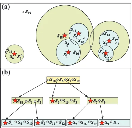
Fig. 1. A schematic view of the DBM-tree: (a) covering radius for subtrees and nodes; and (b) tree node organization. The height of the subtree represented by elements6is shallower than the subtreess18ands7. elementss19,s18(second
level),s16ands3 are not in the last level of the tree.
of the problems mention before, we take a new direction in our research andbreak the paradigm that “good performance is directed correlated to height-balanced trees”.
4. THE DBM-TREE
The DBM-tree is a hierarchical, dynamic structure that grows bottom-up and allows, at any time, new elements to be inserted. Self organizations and node splits can occur in order to accommodate new elements. Basically, when inserting a new element, the tree root is evaluated in order to choose subtrees that can accommodate the new element. There are cases where the new element is inserted in the current node, and not in its subtrees. This process on choosing a node that can accommodate a new element is repeated recursively until a suitable node is found w.r.t. some policy. The DBM-tree has several policies, described in this section, on choosing a suitable node to accommodate a new element, as well as node splitting policies.
The most remarkable difference in the structure, when compared to other structures like the Slim-tree, is that there is no distinction among index and leaf nodes. In this way, elements or subtrees can be stored inany node in any level of the tree. Similar to other MAM, the DBM-tree uses nodes of fixed size in order to optimize data transfer from/to disk. Its main intent is to organize elements in a hierarchical structure using representatives as centers of minimum bounding regions (or balls) that covers all elements in their subtrees. An element can be assigned to a node if the covering radius of the representative covers it. An example of a DBM-tree indexing elements in a 2-dimensional space is shown in Figure 1. In Figure 1(a), 16 elements are represented with small circles, while the representative for a node with a star. The covering radius of each node or subtree is represented with a large circle covering all elements that belong to the node or subtree. The same tree is shown in Figure 1(b), but this time in a tree representation. Note that element s19 in the root node is
an element, not a representative, like s6, s7 ands18. Storing element s19 in the root node prevents
that the subtree represented bys18increases its covering radius to covers19, and thus increasing the
overlapping between subtrees18and its siblingss6 ands7.
Node: [ce,array [1..ce]of {<si, d(srep, si), si.ptr, si.radius>or<si, d(srep, si)>}]
where a node can hold up to c entries. Attribute ce, ce ≤ c, stores the total number of entries (elements or subtrees) stored in a node. Entries can be of two types: subtrees, represented by
<si, d(srep, si), si.ptr, si.radius>, and elements, represented by<si, d(srep, si)>. For subtree entries,
si is the representative for the subtreesi.ptr,si.radiusis the minimum radius that coversall entries in subtreesi.ptr, i.e. ∀s′
i∈si.ptr, si.radius=max(d(si, si′)+s′i.radius), andd(srep, si) is the distance
between the subtree representativesi to the node representativesrep. For element entries, only two fields are required: the element itselfsi with identifiessi.oid, and the distanced(srep, si) betweensi
to the representative of the nodesrep that it belongs to. This distance is stored and used, using the triangle inequality previous described, in order to avoid computing the distance of the element to the query element. All element entries, stored in a particular node, are not covered by any subtree that it belongs to, that is, there is no subtree that can accommodate the element without changing the radius of the subtree. An example of such example is elements19 in Figure 1; there is no subtree in
the root node that accommodate elements19 without changing its radius (subtreess18,s6 ands7).
If an element is chosen to be a representative of its node, then a copy of it is promoted to an immediate level up the tree (unless the node is the root of the tree). This is similar to the promotion process of the B+-tree. For a set of elements in a node, the best local choice for a representative is
the one that has the minimum covering radius. This simple heuristic is used for both Slim-tree and M-tree. The intuition behind it is that, minimizing the radius for a particular node also leads to less covering area among its siblings. Moreover, this heuristic is very easy to implement since updates only occur in the path of insertion.
The DBM-tree self adjust itself when a new element is inserted in the structure. The process of insertion starts from the root of the tree to one node in the tree (top-bottom fashion). This process is recursive in nature and try to find a node that better accommodate the new element. There are two policies on choosing a node, or a subtree, to insert the new element. They are:
—minDist: among all the subtrees that cover the new element, choose the one that has the smallest distance between the representative and the new element. If there is no such subtree, then the element is inserted in the current node;
—minGDist: among all the subtrees that cover the new element, choose the one that has the smallest distance between the representative and the new element. In case there is no such subtree that satisfy this condition, then it is chosen a subtree that has its representative closer to the new element. Thus, in the second condition, the covering radius needs to increase in order to accommodate the new element.
The main difference between these two policies are that, for the first one the flexibility in creating unbalanced trees is more than the second one. That is, if there is no subtree that can accommodate the new element without changing its covering radius, then it is inserted in the current node, no matter the level of the current node. On the other hand, in the second policy whenever the case mention before fails, then a subtree is chosen if its representative is the closest to the new element.
The algorithm to insert new elements is described in Algorithm 1. TheChooseSubtree function returns the most suitable place to insert the new element, based on the policy described above (minDist orminGDist). It starts searching in the root node and proceeds searching recursively for a node that qualifies (that is, the one most appropriated) to store the new elementsnew. The insertion of snew
Algorithm 1Insert
Require: snew: new element to be inserted, ptr: pointer to the subtree wheresnewwill be inserted
1: si←ChooseSubtree(snew, ptr){find a suitable subtree that can accommodatesnew}
2: ifsiis a valid subtreethen
3: promotion←Insert(snew, si.ptr){recursively insertsnewinsisubtree}
4: ifpromotion=true then
5: Update(ptr){update the current node}
6: insert the element set not covered for node split in the current node 7: foreachsjnow covered by the updatedo
8: Demote(sj){demote entries for optimization purposes}
9: end for
10: end if
11: else if ptr.ce< cthen
12: ptr.Add(snew){insertsnew in nodeptr}
13: else
14: SplitNode(snew, ptr){nodeptrdoes not have enough space}
15: returnpromotion{creates a new node, and promotes two representatives for new and old nodes}
16: end if
The policy chosen by the ChooseSubtree function has a big impact in the resultant tree. The minDistoption tends to build trees with small covering radii, but the trees can grow higher than the trees built with the minGDist option. The minGDist option tends to produce shallower trees than those produced with theminDistoption, but with higher overlapping between the subtrees.
If the chosen node does not have enough space to accommodatesnew, then all the existing entries together with the new element must be redistribute between one or two nodes, depending on the redistribution policy of the SplitNodefunction. The SplitNodefunction deletes the node ptr and remove its representative from its parent node. Its former entries and snew are then redistributed between one or more new nodes, and the representatives of the new nodes, together with the set of entries of the former node ptr not covered by the new nodes, are promoted and inserted in the parent node. Notice that the set of entries of the former node that are not covered by any new node can be empty. The DBM-tree has two options to choose the representatives of the new nodes in the SplitNodealgorithm:
—minMax: this option distributes entries into two nodes, allowing a possibly empty set of entries not covered by these two nodes. Each pair of entries is considered as candidate to be the representatives of each new node. For each pair, this algorithm tries to insert each remaining entry into the node having the representative closest to it. The final representatives will be the ones that generated a pair of radii where the largest radius of the pair is the smallest among all possible pairs. The computational complexity of this algorithm isO(c3), wherecis the number of entries to be distribute
between the nodes;
—minSum: this option is similar tominMax, but the two representatives selected is the pair with the smallestsum of the two covering radii.
The minimum node occupation can be between one and half of the node capacityc. If the minimum occupation is set to be half of the node capacity, all thecentries must be distributed between the two new nodes created by theSplitNodealgorithm. After defining the representative of each new node, the remaining entries are inserted in the node with the closest representative. After distributing every entry, if one of the two nodes stores only its representative, then this node is destroyed and its sole entry is inserted in its parent node. Based on the experiments and in the literature [Ciaccia et al. 1997], splits leading to an uneven number of entries in the nodes can be better than splits with equal number of entries in each node, because it tends to minimize the overlapping regions between the two nodes.
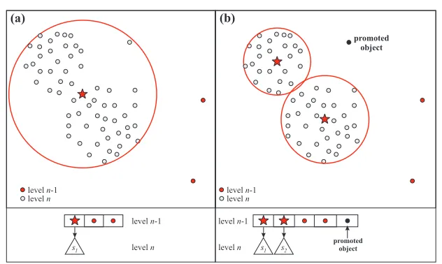
Fig. 2. In order to accommodate two new elements (represented as bold circles), the node in (a) needs to be split into two. Because three elements (represented in bold in (b)) are in an area with low element density, including them in any of the two new nodes it generates to much overlapping between these two nodes, and also triggers more overlapping in other parts of the tree (not shown here).
filled with this minimum number of entries. After this, the remaining entries will be inserted into the node only if its covering radius does not increase the overlapping regions between the two. The rest of entries, that were not inserted into these two nodes, are inserted in the parent node.
Splittings promote the representative to the parent node, which in turn can cause other splittings. After the split propagation or the update of the representative radii, it can occur that former uncovered single element entries are now covered by the updated subtree. In this case each of these entries is removed from the current node and reinserted into the subtree that covers it (Demote). Figure 2 illustrates a node configuration (a) before and (b) after a split. It is possible to see that if any of the three elements promoted (bold circles) were included in any of the two new nodes (represented with a large circle for its covering radius and star for its representative), then the overlap would be very large among these two nodes. Moreover, this expansion could trigger much more overlapping in their siblings and parents. Instead, we let these three elements that are in a low density area to be included in a node belonging in a higher level in the tree.
4.1 Similarity Queries on DBM-tree
Here we describe the two main similarity queries implemented in the DBM-tree: Range query (RQ) and k-Nearest Neighbor query (kN N Q). Both queries work in a similar way as the ones in the Slim-tree and M-tree. We describe both algorithms here for informative purposes. The only major difference among the algorithms is in thekNNQalgorithm for the DBM-tree. This difference is detailed next.
Algorithm 2RQ
Require: ptrtree to be perform the search, query elementsqand query radiusrq
1: foreachsi∈ptr do
2: {use the triangle inequality first}
3: if|d(srep, sq)−d(srep, si)| ≤rq+si.radiusthen
4: dist←d(si, sq){compute distance}
5: ifdist≤rq+si.radiusthen
6: ifsiis a subtreethen
7: RQ(si.ptr, sq, rq){recursively analyze subtreesi.ptr}
8: else
9: R.Add(si){add elementsito the result setR}
10: end if
11: end if
12: end if 13: end for
ThekNNQ algorithm requires a dynamic radiusrk to perform the pruning. In the beginning of the processrk is set to a value that covers all the indexed elements. rk is adjusted with a smaller new radius afterk elements are inserted in R. After this, whenever a swap occurs, rk is adjusted again with a new smaller radius, e.g. the biggest distance of all elements inRto the query element. A swap happens if an element closer to the query element is found and this distance is smaller than any entry inR. This principle is also applied in both Slim-tree and M-tree. The only main difference between the DBM-tree and these two structures is related to the evaluation order of entries in node ptr. In order to fast shrinkrk, entries that are elements in node ptrare analyzed first, then its subtrees are further analyzed in a second step. ThekNNQ algorithm uses this two distinct phases mainly because the rate thatrk adjusts to the optimal value1 interferes in the performance of thekN N Qalgorithm.
We do not show the experiments of this operation in this article, but on average the running time is up to 18% faster using the two phases analyzes.
4.2 TheShrinkOptimization Algorithm
We also propose a post-optimization algorithm for already built DBM-trees called Shrink. This algorithm aims at “shrinking” the nodes by exchanging entries between nodes in order to reduce the amount of overlapping between subtrees. Reducing overlapping regions improves the structure query performance, which results in decreasing of the number of distance calculations, total processing time and, mainly, the number of disk accesses required to answer bothRQandkN N Qqueries. TheShrink algorithm can be executed at any time during the evolution of a DBM-tree, for example, after the insertion of many new elements.
TheShrink algorithm is described in Algorithm 3. The optimization process is applied in every node of a DBM-tree. The stop condition for this algorithm occurs in two cases: when there is no entry exchanges in a previous iteration; or when the number of exchanges already performed is larger than 3 times the total number of entries in the node. This latter condition assures that no cyclic exchanges can lead to a dead loop. After performing some experiments we observed that increasing this number to a bigger value does not improve too much the structure. For each entrysi in node
ptr, the algorithm searches for another entrysj that covers the farthest entrysi.farthest from si. If such node exists, then entrysi.farthest is remove fromsi and inserted insj. If after some exchanges nodesi become empty, thensiis removed from the structure. After these exchanges, the information associated tosi and sj needs to be updated in ptr node. During the exchanging of entries between nodes, some nodes can retain just one entry, so they are promoted and the empty node is deleted from the structure, further improving the performance of the search operations over the tree.
1the optimalr
Algorithm 3Shrink
Require: ptr: root of the tree to be optimized
1: exchanges←0{variable used to count the total number of exchanges}
2: changed←true{variable used to check if an exchange was performed}
3: {default value ofMAXEX is set to 3}
4: whileexchanges≤MAXEX ∗ptr.ceandchanged=true do
5: changed←false
6: foreach subtreesi∈ptrdo
7: letsi.farthest be the farthest entry insifrom its representative
8: foreach entrysj∈ptrandsi6=sjdo
9: ifd(sj, si.farthest≤sj.radiusandsj.ce< cthen
10: {nodesjcoverssi.farthestand has space to store it}
11: si.Remove(si.farthest){remove entrysi.farthestfromsi}
12: sj.Add(si.farthest){insert entrysi.farthestinsj}
13: si.U pdateRadius(){update radius of subtreesi}
14: sj.U pdateRadius(){update radius of subtreesj}
15: changed←true
16: exchanges←exchanges+ 1
17: end if
18: end for
19: ifnodesi.ce= 0then
20: Delete(si.ptr){delete nodesi.ptrfrom the tree}
21: ptr.Remove(si){remove entrysifromptr}
22: end if
23: end for 24: end while
25: {part to remove single entries inptr.si}
26: foreach subtreesi∈ptrdo
27: ifnodesi.ce= 1then
28: Delete(si.ptr){delete nodesi.ptrfrom the tree}
29: ptr.U pdate(si){update entrysifrom subtree to element inptr}
30: end if 31: end for
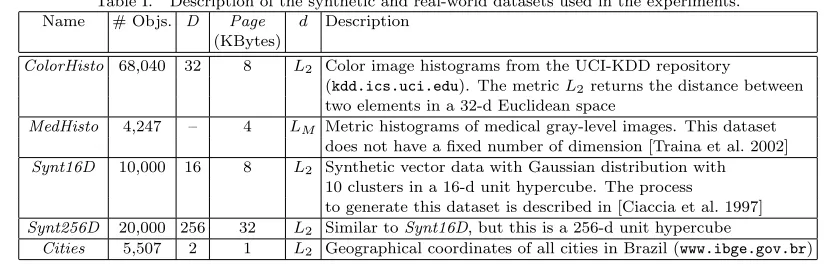
Table I. Description of the synthetic and real-world datasets used in the experiments. Name # Objs. D Page d Description
(KBytes)
ColorHisto 68,040 32 8 L2 Color image histograms from the UCI-KDD repository
(kdd.ics.uci.edu). The metricL2returns the distance between
two elements in a 32-d Euclidean space
MedHisto 4,247 – 4 LM Metric histograms of medical gray-level images. This dataset
does not have a fixed number of dimension [Traina et al. 2002] Synt16D 10,000 16 8 L2 Synthetic vector data with Gaussian distribution with
10 clusters in a 16-d unit hypercube. The process
to generate this dataset is described in [Ciaccia et al. 1997] Synt256D 20,000 256 32 L2 Similar toSynt16D, but this is a 256-d unit hypercube
Cities 5,507 2 1 L2 Geographical coordinates of all cities in Brazil (www.ibge.gov.br)
5. EXPERIMENTAL EVALUATION
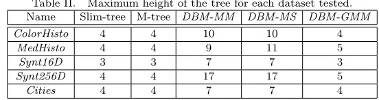
Table II. Maximum height of the tree for each dataset tested. Name Slim-tree M-tree DBM-MM DBM-MS DBM-GMM
ColorHisto 4 4 10 10 4
MedHisto 4 4 9 11 5
Synt16D 3 3 7 7 3
Synt256D 4 4 17 17 5
Cities 4 4 7 7 4
The computer used for the tests is an Intel Pentium 4 1.6GHz processor with 512 MB of RAM and 40 GB of disk space, running Microsoft Windows 2000. All three structures (DBM-tree, Slim-tree and M-Slim-tree) were implemented using the C++ language into the Arboretum MAM library (www.gbdi.icmc.usp.br/arboretum), all with the same code optimization, to obtain a fairly com-parison. The DBM-tree was compared with the well-known, most efficient and used dynamics MAM so far: Slim-tree and M-tree.
The Slim-tree and the M-tree were set up using their best recommended setups. They are: minDist for theChooseSubtreealgorithm,minMax for the split algorithm and the minimal occupation set to 25% of node capacity. The results for the Slim-tree were measured after the execution of the Slim-Down optimization algorithm. We evaluated three configurations for the DBM-tree, all with minimal occupation set to 30% of node capacity, which are the following:
—DBM-MM:minDistpolicy forChooseSubtreeandminMaxforSplitNodemethod; —DBM-MS:minDistpolicy forChooseSubtreeandminSumforSplitNodemethod; —DBM-GMM:minGDistpolicy forChooseSubtreeandminMaxforSplitNodemethod.
We extracted 500 elements for each dataset to generate query centers. They were randomly chosen from each dataset, where half of them (250) were removed from the dataset before creating the trees, and the other half were duplicated in the query set (this last half set is in the tree and the query set). Hence, half of the queries in the query set are indexed in a DBM-tree and the other half are not. This allows us to evaluate queries that are indexed and not. Each dataset were used to build one tree of each type, and every tree was built inserting one element at a time, calculating the average number of distance calculations, average number of disk accesses and total processing time (in seconds). In the plots of measurements, each point corresponds to performing 500 queries with the same parameters but varying query centers. The value forkvaries from 2 to 20 for each measurement, and the radius for
kN N Qvaries from 0.1% to 10% of the largest distance between pairs of elements in the dataset. We chosen these range of values for both queries because they are the most meaningful values used when performing similarity queries. TheRQgraphics are inlog scale for the radius abscissa to emphasize the relevant part of the graph. All measurements were performed after the execution of theShrink algorithm.
The building time, maximum height and the distribution of elements in the structure were measured for every tree. The building time of all 5 trees were similar for each dataset. It is interesting to compare the maximum height of all DBM-trees with the balanced trees, so they are summarized in Table II.
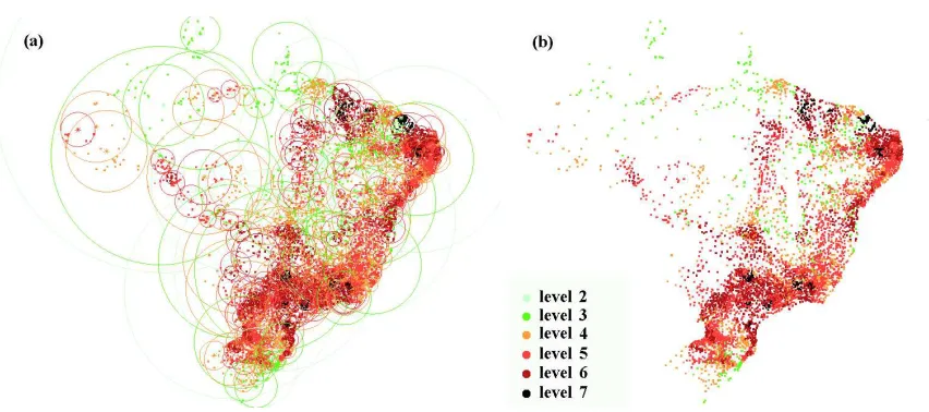
Fig. 3. Visualization of theDBM-MM structure for theCitiesdataset. (a) with the covering radius of the nodes; and (b) only the elements. It is possible to verify that the structure is deeper (darker elements) in high-density regions, and shallower (lighter elements) in low-density regions.
The data distribution across the levels of a DBM-tree is shown in Figure 3 using theCitiesdataset. This is only possible because this dataset is in a 2-dimensional Euclidean space. Figure 3 shows the elements indexed in aDBM-MM with different color representing elements at different levels of the tree. Figure 3(a) shows all elements and the covering radius of each node in the tree, and Figure 3(b) shows only the elements in the tree. The elements with darker colors (red and black) are in a deeper level than those with lighter colors (green). The depth of the tree is larger in higher density regions and that elements are stored in every level of the structure, as expected. It visually shows that the depth of the tree is smaller in low density regions, and that the number of elements at the deepest levels is small, even in the high-density regions.
5.1 Performance Comparison
We have used many synthetic and real datasets to evaluate the performance of the DBM-tree. We now present the results obtained when comparing the DBM-tree with the best setup of the Slim-tree and M-Slim-tree. Due to space limitations we only present the results from four meaningful datasets (ColorHisto, MedHisto, Synt16D and Synt256D), which are high-dimensional and non-dimensional (metric) datasets, and gives a fair sample of the behavior of each structure. The main motivation in these experiments is to evaluate the performance of the DBM-tree with its best competitors with respect to the 2 main similarity queries: RQandkN N Q.
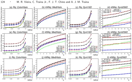
Figure 4 shows the measurements to answer RQ and kN N Q on 4 datasets. The graphs on the first row (Figures 4(a-d)) show the average number of distance calculations. It is possible to note in these graphs that every DBM-tree executed on average less distance calculations than the Slim-tree and M-tree. Among all, theDBM-MS presented the best result for almost every dataset, losing only at theSynt256D dataset to DBM-GMM. None of the DBM-trees executed, for every dataset, more distance calculations than the Slim-tree or the M-tree. The graphs also show that the DBM-tree reduces the average number of distance calculations up to 67% for RQ (graph (c)) and up to 35% for kN N Q (graph (d)), when compared to the Slim-tree, which is the best balanced tree in every dataset wrt distance calculations. When compared to M-tree, the DBM-tree reduced up to 72% for
RQ(graph (c)) and up to 41% forkN N Q(graph (d)).
The graphs of the second row (Figures 4(e-h)) show the average number of disk accesses for both
250 300 350 400 450 500 550 600 650
0.0001 0.001 0.01 0.1 1
radius 1000 1500 2000 2500 3000 3500 4000 4500 5000 5500
0.0001 0.001 0.01 0.1 1
radius 350 400 450 500 550 600 650 700 750 800 850
2 4 6 8 10 12 14 16 18 20
k 80 90 100 110 120 130 140 150 160
2 4 6 8 10 12 14 16 18 20
k 7 8 9 10 11 12 13 14 15 16 17
2 4 6 8 10 12 14 16 18 20
k 4 6 8 10 12 14 16 18
0.0001 0.001 0.01 0.1 1
radius 0.1 0.2 0.3 0.4 0.5 0.6 0.7
0.0001 0.001 0.01 0.1 1
radius 0 100 200 300 400 500 600 700 800
0.0001 0.001 0.01 0.1 1
radius 10 15 20 25 30 35 40
0.0001 0.001 0.01 0.1 1
radius 80 100 120 140 160 180 200 220
2 4 6 8 10 12 14 16 18 20
k 5 6 7 8 9 10 11 12 13
2 4 6 8 10 12 14 16 18 20
k 350 400 450 500 550 600 650 700 750 800
2 4 6 8 10 12 14 16 18 20
k (e)Rq: ColorHisto
(a)Rq: ColorHisto (b)kNNq: MedHisto
(f)kNNq: MedHisto
(j)kNNq: MedHisto
(i)Rq: ColorHisto (k)Rq: Synt16D
(c)Rq: Synt16D
(g)Rq: Synt16D (h)kNNq: Synt256D
(l)kNNq: Synt256D
(d)kNNq: Synt256D
M-Tree Slim-Tree DBM-MM DBM-MS DBM-GMM A
vg Number of Dist
ance Calculation A vg of Disk Access Number T ot al T ime (s) T ot al T ime (s) T ot al T ime (s) T ot al T ime (s) A
vg Number of Disk
Access
A
vg Number of Disk
Access
A
vg Number of Disk
Access
A
vg Number of Dist
ance Calculation
A
vg Number of Dist
ance Calculation
A
vg Number of Dist
ance Calculation M-Tree Slim-Tree DBM-MM DBM-MS DBM-GMM M-Tree Slim-Tree DBM-MM DBM-MS DBM-GMM M-Tree Slim-Tree DBM-MM DBM-MS DBM-GMM M-Tree Slim-Tree DBM-MM DBM-MS DBM-GMM M-Tree Slim-Tree DBM-MM DBM-MS DBM-GMM M-Tree Slim-Tree DBM-MM DBM-MS DBM-GMM M-Tree Slim-Tree DBM-MM DBM-MS DBM-GMM M-Tree Slim-Tree DBM-MM DBM-MS DBM-GMM M-Tree Slim-Tree DBM-MM DBM-MS DBM-GMM M-Tree Slim-Tree DBM-MM DBM-MS DBM-GMM M-Tree Slim-Tree DBM-MM DBM-MS DBM-GMM
Fig. 4. Comparison of the average number of distance calculations (first row), average number of disk accesses (second row) and total processing time (ins) (third row) of DBM-tree, Slim-tree and M-tree, forRQandkN N Qqueries for the ColorHisto((a), (e) and (i) -RQ),MedHisto((b), (f) and (j) -kN N Q),Synt16D((c), (g) and (k) -RQ) andSynt256D ((d), (h) and (l) -kN N Q) datasets.
and the M-tree. The graphs show that the DBM-tree reduces the average number of disk accesses up to 43% forRQ(graph (g)) and up to 35% forkN N Q(graph (h)), when compared to the Slim-tree. It is important to note that the Slim-tree is the MAM that in general requires the lowest number of disk accesses between every previous published MAM. These measurements were taken after the execution of theSlim-Downalgorithm in the Slim-tree. When compared to the M-tree, the gain is even greater, increasing to up to 54% forRQ(graph (g)) and up to 42% forkN N Q(graph (h)).
An important observation is that the immediate result of decreasing overlap among nodes of a tree is the reduced number of distance calculations. However, the number of disk accesses in a MAM is also related to the overlapping between subtrees. An immediate consequence of this fact is that decreasing the overlap reduces both the number of distance calculations and of disk accesses, to answer both types of similarity queries. These two benefits contribute to reduce the total processing time of queries.
The graphs of the third row (Figures 4(i-l)) show the total processing time in seconds. As the three DBM-trees performed lesser distance calculations and disk accesses than both Slim-tree and M-tree, they are naturally faster to answer bothRQ andkN N Q. The importance of comparing query time is that it reflects the total complexity of the algorithms besides the number of distance calculations and the number of disk accesses. The graphs shows that the DBM-tree is up to 44% faster to answer
RQandkN N Q(graphs (k) and (l)) than Slim-tree. When compared to the M-tree, the reduction in total query time is greater, going to be up to 50% forRQandkN N Q queries (graphs (k) and (l)).
5.2 Experiments regarding theShrinkAlgorithm
550 600 650 700 750 800 850 900 950 1000 1050 1100
2 4 6 8 10 12 14 16 18 20
k (b)kNNq: ColorHisto
A
vg Number of Disk
Access 250 300 350 400 450 500 550 600
0.0001 0.001 0.01 0.1 1
DBM-MM DBM-MS DBM-GMM DBM-MM - Shrink DBM-MS - Shrink DBM-GMM - Shrink
DBM-MM DBM-MS DBM-GMM DBM-MM - Shrink DBM-MS - Shrink DBM-GMM - Shrink
DBM-MM DBM-MS DBM-GMM DBM-MM - Shrink DBM-MS - Shrink DBM-GMM - Shrink
DBM-MM DBM-MS DBM-GMM
DBM-MM - Shrink DBM-MS - Shrink DBM-GMM - Shrink
radius (a)Rq: ColorHisto
A
vg Number of Disk
Access
radius (c)Rq: Synt16D
A
vg Number of Disk
Access 10 15 20 25 30 35 40
0.0001 0.001 0.01 0.1 1
k (d)kNNq: Synt16D
A
vg Number of Disk
Access 32 34 36 38 40 42 44 46 48 50 52
2 4 6 8 10 12 14 16 18 20
Fig. 5. Average number of disk accesses to performRQand kN N Q queries in the DBM-tree before and after the execution of theShrinkalgorithm: (a)RQonColorHisto, (b)kN N QonColorHisto, (c)RQonSynt16D, (d)kN N Q
onSynt16D. 200 400 600 800 1000 1200 1400 1600 1800 2000
1 2 3 4 5 6 7 8 9 10
# of dataset elements(x10K) # of dataset elements (x10K) # of dataset elements (x10K) # of dataset elements (x10K)
(a)kNNq: Synt16D - k=10
1 2 3 4 5 6 7
1 2 3 4 5 6 7 8 9 10
(c)kNNq: Synt16D - k=10
0 50 100 150 200 250 300 350
1 2 3 4 5 6 7 8 9 10
(b)kNNq: Synt16D - k=10
T ot al T ime (s) T ot al T ime (s) A
vg Number of Disk
Access
A
vg Number of Dist
ance Calculation DBM-MM DBM-MS DBM-GMM DBM-MM DBM-MS DBM-GMM DBM-MM DBM-MS DBM-GMM DBM-MM DBM-MS DBM-GMM
(d)Rq: Synt16D - radius=0.1%
0.5 1.0 1.5 2.0 2.5 3.0 3.5 4.0 4.5 5.0 5.5
1 2 3 4 5 6 7 8 9 10
Fig. 6. Scalability of all three DBM-trees regarding the dataset size indexed duringkN N Q((a) and (b)) andRQ((c) and (d)), The dataset indexed was theSynt16Dwith 100,000 elements.
other datasets tested. Because the greater benefit of the Shrink algorithm is reducing the number of disk accesses for queries, we only report this measurements here. Figures 5(a) forRQand (b) for
kN N Qrepresents the results for theColorHistodataset, and Figures 5(c) forRQand (d) forkN N Q
for theSynt16D dataset.
Figure 5 compares the query performance before and after the execution of theShrinkalgorithm for DBM-MM,DBM-MS andDBM-GMM for bothRQ andkN N Q. The performance of the Slim-tree (after ran the Slim-Down) and M-tree are also shown in the figures. Every graph shows that the Shrink algorithm improves the final trees. The most expressive result is theDBM-GMM indexing theSynt16D, which achieved up to 30% lesser disk accesses forkN N QandRQas compared with the same structure not optimized.
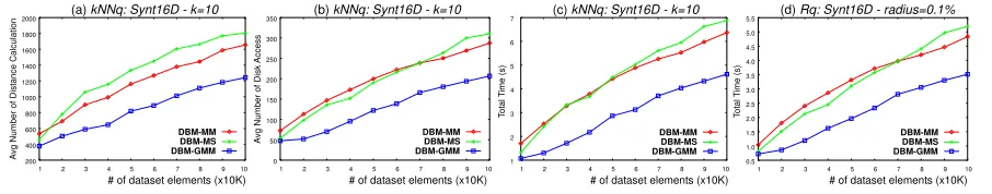
5.3 Scalability of the DBM-tree
In the last set of experiments we evaluated the behavior of the DBM-tree regarding scalability when increasing the number of elements indexed. To do so, we generated 10 datasets similar to theSynt16D, each one with 10,000 elements. We inserted all 10 datasets in the same tree, totaling 100,000 distinct elements. After inserting each dataset we run sets of queries, executing 500 similarity queries for each point in the graph. The behavior was equivalent for different values ofkand radius, thus we present only the results fork=10 and radius=0.1%.
Figure 6 presents the behavior of the three DBM-tree considering: the average number of distance calculations (first row), disk accesses (second row), and total running time (third row) for kN N Q
6. CONCLUSIONS
This paper presents a new dynamic MAM called DBM-tree (Density-Based Metric tree), which in a controlled way relaxes the height-balancing requirement of access methods, trading a controlled amount of unbalancing at denser regions of the dataset for a reduced overlapping among subtrees. This is the first dynamic MAM that makes possible to reduce the overlap between nodes relaxing the rigid balancing of the structure. The height of the tree is higher in denser regions, in order to keep a tradeoff between breadth-searching and depth-searching. The options to define how to construct a tree and the optimizations possibilities in DBM-tree are larger than in rigid balanced trees, because it is possible to adjust the tree according to the data distributions at different regions of the data space. Therefore, this paper also presented a new optimization algorithm, calledShrink, which improves the performance in trees reorganizing the elements among their nodes.
The experiments performed over synthetic and real datasets showed that theDBM-treeoutperforms the main balanced structures existing so far: the Slim-tree and the M-tree. In average, it is up to 50% faster than the traditional MAM and reduces the number of required distance calculations to up to 72% when answering similarity queries. The DBM-tree spends fewer disk accesses than the Slim-tree, that until now was the most efficient MAM with respect to the number of disk accesses. The DBM-tree requires up to 54% fewer disk accesses than the balanced trees. After performed theShrink algorithm, its performance achieves improvements up to 30% for range andk-nearest neighbor queries considering disk accesses. It was also shown that the DBM-tree scales up very well with respect to the number of elements indexed, presenting sub-linear behavior, which makes it well-suited to very large datasets.
Among the future works, we intend to develop a bulk-loading algorithm for the DBM-tree. As the construction possibilities of the DBM-tree is larger than those of the balanced structures, a bulk-loading algorithm can employ strategies that can achieve better performance than is possible in other trees. Other future work is to develop an element-deletion algorithm that can really remove elements from the tree. All existing rigidly balanced MAM such as the Slim-tree and the M-tree, cannot effectively delete elements being used as representatives, so they are just marked as removed, without releasing the space occupied, so it remains being used in the comparisons required in the search operations. The organizational structure of the DBM-tree enables the effective deletion of elements, making it a completely dynamic MAM.
REFERENCES
Baeza-Yates, R. A.,Cunto, W.,Manber, U.,and Wu, S.Proximity matching using fixed-queries trees. InProceedings
of the Annual Symposium on Combinatorial Pattern Matching. Cancun, Mexico, pp. 198–212, 1994.
Bayer, R. and McCreight, E. M. Organization and maintenance of large ordered indexes. Acta Informatica1 (3):
173–189, 1972.
Beckmann, N.,Kriegel, H.-P.,Schneider, R.,and Seeger, B.The R*-tree: An efficient and robust access method
for points and rectangles. InProceedings of the ACM SIGMOD Int’l Conference on Management of Data Conference. ACM Press, Atlantic City, USA, pp. 322–331, 1990.
Bentley, J. L. and Friedman, J. H.Data structures for range searching. ACM Computing Surveys11 (4): 397–409,
1979.
Beyer, K. S.,Goldstein, J.,Ramakrishnan, R.,and Shaft, U. When is “nearest neighbor” meaningful? In
Pro-ceedings of the Int’l Conference on Database Theory. Lecture Notes in Computer Science, vol. 1540. Springer-Verlag, pp. 217–235, 1999.
B¨ohm, C.,Berchtold, S.,and Keim, D. A.Searching in high-dimensional spaces: Index structures for improving the
performance of multimedia databases.ACM Computing Surveys33 (3): 322–373, 2001.
Bozkaya, T. and ¨Ozsoyoglu, M. Distance-based indexing for high-dimensional metric spaces. InProceedings of the
ACM SIGMOD Int’l Conference on Management of Data Conference. Tucson, USA, pp. 357–368, 1997.
Bozkaya, T. and ¨Ozsoyoglu, M. Indexing large metric spaces for similarity search queries.ACM Trans. on Database
Systems24 (3): 361–404, 1999.
Brin, S.Near neighbor search in large metric spaces. InProceedings of the Int’l Conference on Very Large Data Bases.
Burkhard, W. A. and Keller, R. M. Some approaches to best-match file searching. Communications of the ACM16 (4): 230–236, 1973.
Chavez, E.,Navarro, G.,Baeza-Yates, R.,and Marroqu´ın, J. L. Searching in metric spaces. ACM Computing
Surveys33 (3): 273–321, 2001.
Ciaccia, P.,Patella, M.,and Zezula, P. M-tree: An efficient access method for similarity search in metric spaces.
InProceedings of the Int’l Conference on Very Large Data Bases. Athens, Greece, pp. 426–435, 1997.
Comer, D.The ubiquitous B-tree. ACM Computing Surveys11 (2): 121–137, 1979.
Faloutsos, C.Searching Multimedia Databases by Content. Kluwer Academic Publishers, Boston, USA, 1996.
Gaede, V. and G¨unther, O.Multidimensional access methods. ACM Computing Surveys30 (2): 170–231, 1998.
Guttman, A. R-tree : A dynamic index structure for spatial searching. InProceedings of the ACM SIGMOD Int’l
Conference on Management of Data Conference. Boston, USA, pp. 47–57, 1984.
Hjaltason, G. R. and Samet, H. Index-driven similarity search in metric spaces. ACM Trans. on Database
Sys-tems28 (4): 517–580, 2003.
Santos, R. F., F.,Traina, A. J. M.,Traina Jr., C.,and Faloutsos, C. Similarity search without tears: The omni
family of all-purpose access methods. InProceedings of the IEEE Int’l Conference on Data Engineering. Heidelberg, Germany, pp. 623–630, 2001.
Sellis, T. K.,Roussopoulos, N.,and Faloutsos, C. The R+-tree: A dynamic index for multi-dimensional objects.
InProceedings of the Int’l Conference on Very Large Data Bases. Morgan Kaufmann Publishers, Brighton, England, pp. 507–518, 1987.
Traina, A. J. M.,Traina Jr., C.,Bueno, J. M.,and de A. Marques, P. M. The metric histogram: A new and
efficient approach for content-based image retrieval. In IFIP Visual Database Systems. Brisbane, Australia, pp. 297–311, 2002.
Traina Jr., C.,Traina, A. J. M.,Faloutsos, C.,and Seeger, B.Fast indexing and visualization of metric datasets
using Slim-trees.IEEE Trans. on Knowledge and Data Engineering14 (2): 244–260, 2002.
Traina Jr., C.,Traina, A. J. M.,Seeger, B.,and Faloutsos, C. Slim-trees: High performance metric trees
mini-mizing overlap between nodes. InProceedings of the Int’l Conference on Extending Database Technology. Konstanz, Germany, pp. 51–65, 2000.
Uhlmann, J. K.Satisfying general proximity/similarity queries with metric trees.Information Processing Letters40 (4):
175–179, 1991.
Vieira, M. R.,Traina Jr., C.,Chino, F. J. T.,and Traina, A. J. M.DBM-tree: A dynamic metric access method
sensitive to local density data. InProceedings of the Brazilian Symposium on Databases. Bras´ılia, Brazil, pp. 163–177, 2004.
Yianilos, P. N. Data structures and algorithms for nearest neighbor search in general metric spaces. InProceedings