www.adv-radio-sci.net/10/333/2012/ doi:10.5194/ars-10-333-2012
© Author(s) 2012. CC Attribution 3.0 License.
Radio Science
FMCW sparse array imaging and
restoration for microwave gauging
S. Kolb and R. Stolle
University of Applied Sciences Augsburg, An der Hochschule 1, 86161 Augsburg, Germany Correspondence to: S. Kolb ([email protected])
Abstract. The application of imaging radar to microwave level gauging represents a prospect of increasing the reliabil-ity of target detection. The aperture size of the used sensor determines the underlying azimuthal resolution. In conse-quence, when FMCW-based multistatic radar (FMCW: fre-quency modulated continuous wave) is used, the number of antennas dictates this essential property of an imaging sys-tem. The application of a sparse array leads to an improve-ment of the azimuthal resolution by keeping the number of array elements constant with the cost of increased side lobe level. Therefore, ambiguities occur within the imaging pro-cess. This problem can be modelled by a point spread func-tion (PSF) which is common in image processing. Hence, an inverse system to the imaging system is needed to restore unique information of existing targets within the observed radar scenario.
In general, the process of imaging is of ill-conditioned nature and therefore appropriate algorithms have to be ap-plied. The present paper first develops the degradation model, namely PSF, of an imaging system based on a uni-form linear array in time domain. As a result, range and azimuth dimensions are interdependent and the process of imaging has to be reformulated in one dimension. Matrix-based approaches can be adopted in this way. The sec-ond part applies two computational methods to the given in-verse problem, namely quadratic and non-quadratic regular-ization. Notably, the second one exhibits an ability to sup-press ambiguities. This can be demonstrated with the results of both, simulations and measurements, and enables sparse array imaging to localize point targets more unambiguously.
1 Introduction
Industrial level gauging by means of microwaves offers a reliable and accurate method to determine the fill level of a reservoir. In most cases the microwave level gauge is a monostatic radar system. This becomes a problem when metallic fixtures like pipes or the enclosure impede detect-ing backscatterdetect-ing from volume surface. In order to improve the robustness of such systems introducing imaging by beam-steering is very promising. In addition, using more than one measurement dimension offers the possibility for estimating levels of non-planar surfaces.
Due to practical aspects, a switched approach using digital beam-forming (DBF) in conjunction with an antenna array will be preferred versus one mechanical panned antenna. In the following this method will be referred to as multistatic radar in which transmitting and receiving elements are co-located. Aiming to continue using the established concept of frequency modulated continuous wave (FMCW) with advan-tages, as for instance a straightforward RF hardware and a good range resolution (Stove, 1992), transmission of a single waveform at each antenna is supposed.
The ability to distinguish between two closely spaced tar-gets is an essential characteristic of an imaging radar and de-pends on the aperture size used. In order to achieve a high angular resolution the array aperture must be large. Mostly, the number of antenna elements is a small number, meaning spacing of the antenna array becomes comparatively wide. As a result, such a sparse antenna array has a high side lobe response generating artefacts in the angular domain.
In general, such an imaging system with DBF can be represented by a convolution of the beam-pattern hant and
Eq. (1) inside the observed area3.
y(ϕ)=
Z
3
hant(ϕ,ϕ)˜ ·x(ϕ)˜ dϕ˜ (1)
In consequence, impulse responsehant is the origin of am-biguities and loss of resolution within a linear imaging cess. A comparable issue is known in theory of image pro-cessing in which degradation of a recorded image is de-scribed by a point spread function (PSF) (e.g. Bertero et al., 1998). In order to improve the quality of an image, the con-cept of deconvolution as an inverse process of imaging is used. This was already applied to enhance angular resolution within an imaging system with mechanical beam-steering (Kolb et al., 2010).
The present paper utilizes existing methods of image pro-cessing to reduce degenerating and ambiguous effects of a sparse array imaging system. The general method is first to express the forward problem which describes how to get the measurable data of an observed radar scene (Bertero et al., 1998). This is shown in Sect. 2 with respect to an antenna ar-ray with DBF. The second step deals with the corresponding inverse problem and its solution by regularization methods to restore unambiguously information of a radar scene. Two es-sential methods are applied to simulation data in Sect. 3 and measurement data in Sect. 4.
2 Direct problem: modelling FMCW sparse array imaging
Due to the architecture of a particular RF frontend, more or less DBF setups are feasible. For reasons of specification, a measurement matrix S can be defined that relates transmit-ting channelsaand receiving channelsb=S·a. Table 1 in-dicates different options for those signal paths available for processing.
A distinction between the following measurement modes is made:
– Reflection and Transmission at/between all elements,
– limited to Reflection only at all elements,
– limited to Transmission only at all elements,
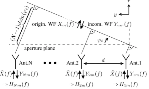
Fig. 1. Array signal model for FMCW beam-forming.
– only one element is able to transmit respectively receive (SIMO/MISO), all others do the opposite.
Without loss of generality, the present paper concentrates on full measurements (Reflection and Transmission) but all considerations could also be used for other modes of measurements.
2.1 Point spread function
Mostly, far-field conditions in gauging situations are ful-filled. In consequence, a plane wavefront (WF) approach, according to Fig. 1, is used to develop an expression of the PSF. Starting from an arbitrary transmitted spectrumX(f )˜
at each single element, a wavefront orthogonal to the beam-direction is generated. Withϕtbeing the direction of a wave-front to and from a potential target, the contributionXm(f )
of them-th element is given by:
Xm(f )= ˜X(f )·exp
−j2πf
c0py,m·sinϕt
, (2)
wherepy,mdenotes they-coordinate of them-th element and c0equals the speed of light, respectively. Looking at an in-coming wavefront from transmitting antennam, the resulting spectrumYnm(f )at receiving antennanbecomes
Ynm(f )=Xm(f )·exp
−j2πf
c0py,n·sinϕt
. (3)
By defining a transfer function as the ratio of received spec-trumYnm(f )over transmitted spectrumX(f )˜ and combining
Eqs. (2), (3), the following expression is found:
Hnm(f )=exp
−j2πf c0
(py,n+py,m)·sinϕt
. (4)
It is desired to generate a wavefront in directionϕt.
There-fore, usually complex weightswnm(f,ϕ) are chosen
com-plex conjugate ofHnm(f ), to realize a delay-and-sum
beam-former.
Fig. 2. Channel model including relevant system components.
centre in the middle of the array (y=0), the output of the beam-former becomes:
AF(f,ϕ)=X
n X
m
Hnm(f )·wnm(f,ϕ), (5)
respectively AF(f,ϕ)=X
n X
m
exp(j2π f dc
0 (n+m−N−1)·(u−ut)), (6)
where the substitutionsu=sinϕ andut=sinϕt are used to
achieve a shift-invariant behaviour. Therefore, Eq. (6) formu-lates the two-dimensional array factor (AF) of an intended point target in directionut=0, which represents the relat-ing transfer function. Consequently, a subsequent inverse Fourier transformaf (r,u)=IFT{AF(f,u)}complies to the impulse response of a target in directionut=0 and range
rt=0.
In case of Reflection and Transmission-variant and a point target at directionut=0 the expression results in:
AF(f,u)=
"
sin(π fduc
0 N )
sin(π fcdu
0 )
#2
. (7)
It is obvious that range-relating domain f and angular-relating domainu are not separable, meaning both dimen-sions are interdependent. This needs to be considered in the process of describing the image process.
In order to take account of all relevant frequency depen-dent effects, remaining components corresponding to Fig. 2 have to be considered. In detail, there are two-way free-space lossα∝ 1
f2 and af-domain windowHwin(f ), possibly used
to suppress ringing in range-domain. According to this de-scription, the PSF inf-domain results in:
PSF(f,u)= 1
f2·AF(f,u)·Hwin(f ). (8)
The PSF in range-domain is finally obtained by an inverse Fourier transform psf(r,u)=IFT{PSF(f,u)}.
Fig. 3. PSF of an X-band FMCW sparse array imaging system with
N=4 single elements and element spacing ofd=40 mm.
In contrast to Eq. (1), the imaging process depends on rangerin addition to the angular domain and has to be com-pleted with the replaced two-dimensional impulse response psf(r,u)of the imaging system to the following expression:
y(r,u)=
Z
3 Z
psf(r− ˜r,u− ˜u)·x(r,˜ u)˜ dr˜du˜ . (9)
To get an idea of the PSF’s effects, Fig. 3 illustrates psf(r,u)
of an X-band (8.2 to 12.4 GHz) FMCW sparse array imag-ing system withN=4 single elements and element spacing of d= 40 mm; seriously violating the half-wavelength rule (λcenter
2 ≈14.6 mm). In consequence of this spatial
undersam-pling, ambiguities against azimuth occur. The applied fre-quency window is of a Hanning characteristic.
2.2 Matrix-vector formulation
For reasons of computational aspects, a finite discrete rep-resentation of Eq. (9) is needed. In this context there is a need to take respect of the interdependent character of both dimensions within the PSF. Hence, in image processing a one-dimensional representation (lexicographic ordering) of two-dimensional data is utilized (e.g. Hunt, 1973), because successively processing of occurring two-dimensional con-volution is illegitimate.
The vector representation of targets versus range and az-imuthx(r,u)∈CNr×Nuis reordered according to
x=hx(1...Nr,1)T,···,x(1...Nr,Nu)T iT
∈CNr·Nu×1, (10) whereNr is the length along range r andNu is the length
riodic character and there is also no other way to define any other boundaries like zero- or reflexive-boundary conditions (see e.g. Nagy et al., 2004). This can also be recognized in the example PSF in Fig. 3 because psf(r,u) does not become 0 foru→ ±∞.
3 Inverse problem: image restoration
The declaration of Eq. (11) gives a description of the imaging behaviour of a FMCW sparse array radar system. With the aim to compute an estimationxˆ of the original scenexfrom the observationzan inverse system is needed. First of all, this can be formulated by a matrix inversion:
ˆ
x=K−1z, (12)
which can also be expressed by a least square (LS) expres-sion (Bertero et al., 1998):
ˆ
x=argmin
x n
kKx−zk2
2 o
. (13)
The LS expression solves the minimization problem but will fail due to ignoring the noise sourcen. In addition, it is com-mon knowledge in image processing that inverse mapping in terms of Eq. (11) is of ill-conditioned nature. This means that there is no unique solution and more appropriate algorithms have to be used to get physically acceptable solutions for the approximation of targetsxˆ.
Generally, constraining the solution provides an opportu-nity to improve the approximation. It is common practice to apply constraints by a functional(x)of the solution to the minimization term Eq. (13) and to use a regularization pa-rameterµ >0 to balance between the residual norm and the solution constraint:
ˆ
x=argmin
x
{kKx−zk22
| {z } residual norm
+µ· (x) | {z } solution norm
}. (14)
The solution constraint is also referred to as solution norm, because a norm is frequently used as a constraining criterion, as described in the following methods.
where L is usually a differential operator, e.g. Laplacian to preserve edges in image processing. Due to the fact, that here point targets are of main interest, the identity matrix L=I is used. By applying a Lagrange multiplier an explicit solution is found and corresponds to a Wiener filter approach (Murli et al., 1999), whose regularization parameter µ complies with inversely proportional value of the occurring signal-to-noise ratio (SNR). Performing a parameter sweep ofµis the subsequent procedure to get a reasonable approximation of targetsxˆ. An appropriate value ofµcan be selected by the L-curve criterion for instance. Therein a parametric log-log plot of residual norm versus solution norm is utilized to de-tect a pounce within the graph (Hansen, 2010).
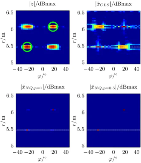
With the intention to verify performance of the CLS method, a noisy channel (SNR≈50 dB) with two point-targets was simulated by a simple time-delay model of Re-flection and Transmission-variant (see Table 1) in Matlab. A linear uniform array with equidistant spacingd=20 mm and
N=7 channels (in plots referred to as full array) is used to form up an antenna array that nearly fits the half-wavelength rule when a frequency range of X-band (see above) is ap-plied. The sparse array raw data (d=40 mm and N=4) is obtained by selecting every second antenna; correspond-ing PSF was shown in Fig. 3. The resultcorrespond-ing Gaussian noise added output of the systemz(r,ϕ) is illustrated in Fig. 4a, whereas factual position of point-targets are shown by green circles. Ambiguities of real existing targets are located quite plainly.
In conjunction with a parameter study of µ the CLS method is applied and a suitable approximation xˆCLS(r,ϕ)
forµ=10−2.5with a logarithmic scaling is shown in Fig. 4b. Obviously, a slight ambiguity suppression can be recognized. An azimuthal sectional view of a selected range cell (high-lighted by gray lines) is given in Fig. 5 and enables stating a suppression of approximately 5 dB in contrast to sparse array data.
3.2 Sparse restoration
Fig. 4. Simulated scenario including regularization approximations (30 dB dynamic with log. colour-mapping applies Fig. 3). (a) Raw data of sparse array, (b) CLS regularization, (c) Sparse regulariza-tion,p=1, (d) Sparse regularization,p=0.5.
Fig. 5. Sectional view of one range cell of simulated data.
Relating to the gauging situation, this can be achieved by uprating of non-sparse solutions ofxˆ, which fits to the fact that mainly a few isolated point targets occur. From a mathe-matical point of view thepnorm solves this particular prob-lem:
kxkp= X
i
|xi|p !1/p
,0< p≤1. (16)
In image processing the utilization of thepnorm is referred
Fig. 6. Isoclines of differentpnorms of the vectorx= [x1,x2]T.
to as non-quadratic (NQ) regularization and formulated by the following modified minimization term (e.g. Cetin, 2001):
ˆ
x=argmin
x
{kKx−zk2
2 | {z } residual norm
+µ· kLxkpp
| {z } solution norm
}. (17)
The rationale behind the p norm is illustrated in Fig. 6 by applying CLS-, 1- and 0.5-norm to a two component vector
x=[x1,x2]T ∈[0,1]. As an example, the marker belongs tox=h1.
√ 2,1.
√
2iT. The 2-norm yields the absolute value of a vector, no matter if the vector is sparse or not. The
pnorm yields similar values if the vector is sparse but much greater values if the vector is dense. In connection with the minimization term Eq. (17) and translated into the inverse problem of imaging this means that a solution with a few number of point targets is preferred to any smooth solution.
In order to test the procedure of NQ regularization to raw data of a sparse array imaging system, same raw data as for CLS regularization is processed for p=1 and p= 0.5, respectively. The utilized algorithm that already han-dles complex-valued problems is described in (Cetin, 2001). Again, a parameter sweep ofµis performed and a manual selection of regularization parameter (µp=1≈0.6, µp=0.5≈
0.3)is done. The results are shown in Fig. 4c and d for both values of p, respectively; sectional view is found in Fig. 5 again. As a result, the side lobe suppression is consider-ably improved for both choices ofpin comparison with CLS method. Especially, in case ofp=0.5 the all over side lobe level reaches a value below the level of the full array as a con-sequence of the sparse regularization approach. A side lobe suppression of approximately 45 dB is achieved and there-fore this approach is well suited to enable a FMCW sparse array imaging system to locate point targets more unambigu-ously.
4 Measurements
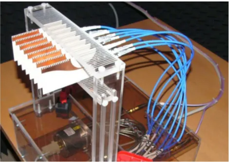
Fig. 7. Switched antenna array for experimental setup.
Fig. 8. Measured scenario including sparse approximation. (30 dB dynamic with log. colour-mapping applies Fig. 3). (a) Raw data of sparse array, (b) Sparse restoration,p=0.5.
to realize a switched multiport measurement system. With regard to the simulation example, 7 antipodal Vivaldi anten-nas (see Fig. 7) were used as single elements of the X-band linear uniform array withd=20 mm to form the full array. Two corner reflectors served as targets and were positioned in front of the array. The distance between sensor and tar-gets is approximately 3.25 m with a slight offset among each other.
The raw data (Fig. 8a) is processed in the same way as sim-ulation data above with CLS and sparse restoration. Figure 9 again illustrates an azimuthal sectional view of a selected range cell view of all restoration methods. Similar to the simulation results applying sparsity to the restoration prob-lem obviously results in good side lobe suppression (p=0.5, Fig. 8b). An attenuation of approximately 45 dB is achieved and is therefore lower than the overall side lobe level of the full array.
Fig. 9. Sectional view of one range cell of measured data.
5 Conclusions
The reliability of a microwave gauging system benefits from the concept of imaging radar. However, an adequate az-imuthal resolution of a FMCW imaging system with a lim-ited number of antennas can only be achieved by apply-ing a sparse antenna array. Consequently, by violatapply-ing the half-wavelength rule, a high side lobe arises and ambiguities within the imaging process occur. By modelling the process of FMCW sparse array imaging using a common wavefront approach, the corresponding PSF was achieved, which has to be inverted to get unambiguously information of real targets. Due to this way of proceeding, the present paper was able to apply two relevant regularization methods from image pro-cessing for the task of restoration. Furthermore, significant improvements in side lobe suppression have been achieved by utilizing sparse restoration for both simulated and mea-sured data of a sparse antenna array.
References
Bertero, M. and Boccacci, P.: Introduction to Inverse Problems in Imaging, Institute of Physics Publishing, Philadelphia, USA, 1998.
Cetin, M. and Karl, W. C.: Feature-enhanced Synthetic Aperture Radar Image Formation Based on Nonquadratic Regularization, IEEE T. Image Process., 10, 623–631, 2001.
Gething, P. J. D.: Radio Direction Finding and Superresolution, Stevenage, England: IEE Electromagnetic Series 4, Peter Pere-grinus, Ltd., 2nd Edn., 1991.
Hansen, P. C.: Discrete Inverse Problems, SIAM, 2010.
Hunt, B. R.: The Application of Constrained Least Squares Estima-tion to Image RestoraEstima-tion by Digital Computer, IEEE T. Com-put., C-22, 805–812, 1973.
Kolb, S., Stolle, R., and Strobel, R.: Microwave Gauging with Im-proved Angular Resolution, European Radar Conference (Eu-RAD) 2010, 192–195, 2010.
ICIAP, 394–399, 1999.
Nagy, J., Ng, M., and Perrone, L.: Kronecker Product Approxima-tions for Image Restoration with Reflexive Boundary CondiApproxima-tions, SIAM J. Matrix Anal. Appl. 25,829–841, 2004.