R E S E A R C H
Open Access
The sinc-Galerkin method and its
applications on singular Dirichlet-type
boundary value problems
Aydin Secer
1*and Muhammet Kurulay
2*Correspondence:
1Department of Mathematical
Engineering, Faculty of Chemical and Metallurgical Engineering, Yildiz Technical University, Davutpasa, ˙Istanbul, 34210, Turkey Full list of author information is available at the end of the article
Abstract
The application of the sinc-Galerkin method to an approximate solution of
second-order singular Dirichlet-type boundary value problems were discussed in this study. The method is based on approximating functions and their derivatives by using the Whittaker cardinal function. The differential equation is reduced to a system of algebraic equationsvianew accurate explicit approximations of the inner products without any numerical integration which is needed to solve matrix system. This study shows that the sinc-Galerkin method is a very effective and powerful tool in solving such problems numerically. At the end of the paper, the method was tested on several examples with second-order Dirichlet-type boundary value problems.
Keywords: sinc-Galerkin method; sinc basis functions; Dirichlet-type boundary value problems;LUdecomposition method
1 Introduction
Sinc methods were introduced by Frank Stenger in [] and expanded upon by him in []. Sinc functions were first analyzed in [] and []. An extensive research of sinc methods for two-point boundary value problems can be found in [, ]. In [, ], parabolic and hy-perbolic problems were discussed in detail. Some kind of singular elliptic problems were solved in [], and the symmetric sinc-Galerkin method was introduced in []. Sinc do-main decomposition was presented in [–] and []. Iterative methods for symmetric sinc-Galerkin systems were discussed in [, ] and []. Sinc methods were discussed thoroughly in []. Applications of sinc methods can also be found in [, ] and []. The article [] summarizes the results obtained to date on sinc numerical methods of computation. In [], a numerical solution of a Volterra integro-differential equation by means of the sinc collocation method was considered. The paper [] illustrates the ap-plication of a sinc-Galerkin method to an approximate solution of linear and nonlinear second-order ordinary differential equations, and to an approximate solution of some lin-ear elliptic and parabolic partial differential equations in the plane. The fully sinc-Galerkin method was developed for a family of complex-valued partial differential equations with time-dependent boundary conditions []. Some novel procedures of using sinc methods to compute solutions to three types of medical problems were illustrated in [], and sinc-based algorithm was used to solve a nonlinear set of partial differential equations in []. A new sinc-Galerkin method was developed for approximating the solution of
tion diffusion equations with mixed boundary conditions on half-infinite intervals in []. The work which was presented in [] deals with the sinc-Galerkin method for solving nonlinear fourth-order differential equations with homogeneous and nonhomogeneous boundary conditions. In [], sinc methods were used to solve second-order ordinary dif-ferential equations with homogeneous Dirichlet-type boundary conditions.
2 Sinc functions preliminaries
LetCdenote the set of all complex numbers, and for allz∈C, define the sine cardinal or sinc function by
sinc(z) = ⎧ ⎨ ⎩
sin(πz)
πz , y= ,
, y= . (.)
Forh> , the translated sinc function with evenly spaced nodes is given by
sinc(k,h)(z) = ⎧ ⎨ ⎩
sin(πz–hkh)
πz–hkh , z=kh, , z=kh.
(.)
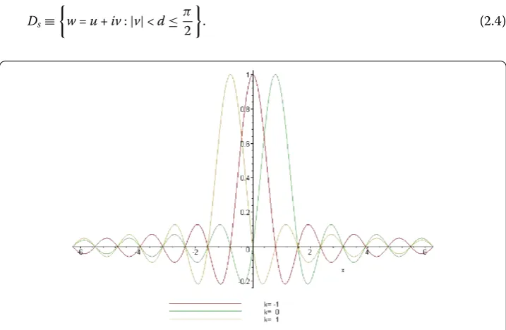
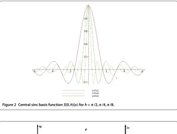
For various values ofk, the sinc basis functionS(k,π/)(x) on the whole real line –∞< x<∞is illustrated in Figure . For various values ofh, the central functionS(,h)(x) is illustrated in Figure .
If a functionf(x) is defined over the real line, then forh> , the series
C(f,h)(x) =
∞
k=–∞
f(kh)sinc
x–kh h
(.)
is called the Whittaker cardinal expansion off whenever this series converges. The infinite stripDsof the complexwplane, whered> , is given by
Ds≡
w=u+iv:|v|<d≤π
. (.)
Figure 2 Central sinc basis functionS(0,h)(x) forh=π/2,π/4,π/8.
Figure 3 The relationship between the eye-shaped domainDEand the infinite stripDS.
In general, approximations can be constructed for infinite, semi-infinite and finite inter-vals. Define the function
w=φ(z) =ln
z –z
(.)
which is a conformal mapping fromDE, the eye-shaped domain in thez-plane, onto the
infinite stripDS, where
DE=z=
x+iy:arg
z –z
<d≤π
. (.)
This is shown in Figure .
For the sinc-Galerkin method, the basis functions are derived from the composite trans-lated sinc functions
Sh(z) =S(k,h)(z) =sinc
φ(z) –kh h
Figure 4 Three adjacent membersS(k,h)◦φ(x) whenk= –1, 0, 1 andh=π8of the mapped sinc basis on the interval (0, 1).
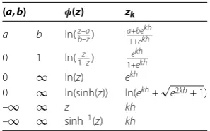
Table 1 Conformal mappings and nodes for some subintervals ofR
(a,b) φ(z) zk
a b ln(z–a b–z)
a+bekh
1+ekh
0 1 ln(1–zz) ekh
1+ekh
0 ∞ ln(z) ekh
0 ∞ ln(sinh(z)) ln(ekh+√e2kh+ 1)
–∞ ∞ z kh
–∞ ∞ sinh–1(z) kh
forz∈DE. These are shown in Figure for real valuesx. The functionz=φ–(w) = e
w
+ew is
an inverse mapping ofw=φ(z). We may define the range ofφ–on the real line as
=φ–(u)∈DE: –∞<u<∞
(.)
the evenly spaced nodes{kh}∞k=–∞on the real line. The image which corresponds to these nodes is denoted by
xk=φ–(kh) =
ekh
+ekh. (.)
A list of conformal mappings may be found in Table [].
Definition . LetDEbe a simply connected domain in the complex planeC, and let∂DE
denote the boundary ofDE. Leta,bbe points on∂DEandφbe a conformal mapDEonto
DSsuch thatφ(a) = –∞andφ(b) = –∞. If the inverse map ofφis denoted byϕ, define
=φ–(u)∈DE: –∞<u<∞
(.)
Definition . LetB(DE) be the class of functionsFthat are analytic inDEand satisfy
ψ(L+u)
F(z)dz→, asu=∓∞, (.)
where
L=
iy:|y|<d≤π
, (.)
and those on the boundary ofDEsatisfy
T(F) =
∂DE
F(z)dz<∞. (.)
The proof of following theorems can be found in [].
Theorem . Letbe(, ),F∈B(DE),then for h> sufficiently small,
F(z)dz–h
∞
j=–∞
F(zj) φ(zj)
= i
∂D
F(z)k(φ,h)(z)
sin(π φ(z)/h) dz≡IF, (.)
where
k(φ,h)z∈∂D=e[iπ φh(z)sgn(Imφ(z))]
z∈∂D=e –πd
h . (.)
For the sinc-Galerkin method, the infinite quadrature rule must be truncated to a finite sum. The following theorem indicates the conditions under which an exponential conver-gence results.
Theorem . If there exist positive constantsα,βand C such that
φF(x)(x)
≤C
⎧ ⎨ ⎩
e–α|φ(x)|, x∈ψ((–∞,∞)),
e–β|φ(x)|, x∈ψ((,∞)), (.)
then the error bound for the quadrature rule(.)is
F(x)dx–h
N
j=–N
F(xj) φ(xj)
≤C
e–αNh
α +
e–βNh β
+|IF|. (.)
The infinite sum in(.)is truncated with the use of(.)to arrive at the inequality(.). Making the selections
h=
πd
αN, (.)
N≡
s αN
β + {
whereJ·Kis an integer part of the statement and N is the integer value which specifies the grid size,then
F(x)dx=h
N
j=–N
F(xj) φ(xj)
+Oe–(π αdN)/. (.)
We used Theorems . and . to approximate the integrals that arise in the formulation of the discrete systems corresponding to a second-order boundary value problem.
Theorem . Letφbe a conformal one-to-one map of the simply connected domain DE
onto DS.Then
δ()jk =S(j,h)◦φ(x)x=x
k=
⎧ ⎨ ⎩
, k=j,
, k=j, (.)
δ()jk =h d dφ
S(j,h)◦φ(x)
x=xk
= ⎧ ⎨ ⎩
, k=j,
(–)k–j (k–j) , k=j,
(.)
δ()jk =h d
dφ
S(j,h)◦φ(x)
x=xk
= ⎧ ⎨ ⎩
–π
, k=j,
–(–)k–j (k–j) , k=j.
(.)
3 The sinc-Galerkin method for singular Dirichlet-type boundary value problems
Consider the following problem:
y+P(x)y+Q(x)y=F(x) (.)
with Dirichlet-type boundary condition
y(a) = , y(b) = , (.)
whereP,QandFare analytic onD. We consider sinc approximation by the formula
y(x)≈yN(x) = N
k=–N
ckS(k,h)◦φ(x), (.)
S(k,h) = sin[ π
h(x–kh)]
π
h(x–kh)
. (.)
The unknown coefficientsckin Eq. (.) are determined by orthogonalizing the residual
with respect to the sinc basis functions. The Galerkin method enables us to determine the ckcoefficients by solving the linear system of equations
LyN–F,S(k,h)◦φ(x)
= , k= –N, –N+ , . . . ,N– ,N. (.)
Letfandfbe analytic functions onDand the inner product in (.) be defined as follows:
f,f=
wherewis the weight function. For the second-order problems, it is convenient to take [].
w(x) =
φ(x). (.)
For Eq. (.), we use the notations (.)-(.) together with the inner product that, given (.) [], showed to get the following approximation formulas:
F(x),S(k,h)◦φ(x)=
w(x)F(x)S(k,h)◦φ(x)dx∼= hwkFk
φk , (.)
Q(x)y(x),S(k,h)◦φ(x)=
w(x)Q(x)y(x)S(k,h)◦φ(x)dx∼=h
wkFk φk
ck, (.)
P(x)y(x),S(k,h)◦φ(x)=
w(x)P(x)y(x)S(k,h)◦φ(x)dx∼=h
wkPk φk
ck
∼= –h
N
j=–N
cj
(Pw) j φ δ
() kj + (Pw)j
δ()kj
h
, (.)
y(x),S(k,h)◦φ(x)=
w(x)y(x)S(k,h)◦φ(x)dx∼=h
wk φk
ck
∼= –h
N
j=–N
cj
w j φδ
() kj +
wj+wjφ
j φj
δ() kj
h +wjφ
j
δkj()
h
, (.)
wherewk=w(xk). If we chooseh= (πd/αN)/andw(x) = /φ(x) as given in [] the
accu-racy for each equation between (.)-(.) will beO(N/e–(πdαN)/).
Using (.), (.)-(.), we obtain a linear system of equations for N+ numbersck.
The N+ linear system given in (.) can be expressed by means of matrices. Letm= N+ , and letSmandcmbe a column vector defined by
Sm(x) =
⎛ ⎜ ⎜ ⎜ ⎜ ⎝
S–N
S–N+
.. . SN ⎞ ⎟ ⎟ ⎟ ⎟
⎠, cm= ⎛ ⎜ ⎜ ⎜ ⎜ ⎝
c–N
c–N+
.. . cN ⎞ ⎟ ⎟ ⎟ ⎟ ⎠. (.)
LetAm(y) denote a diagonal matrix whose diagonal elements arey(x–N),y(x–N+), . . . ,y(xN)
and non-diagonal elements are zero, and also letIm(),Im()andIm()denote the matrices
Im()= ⎡ ⎢ ⎢ ⎢ ⎢ ⎢ ⎢ ⎢ ⎣ · · · · · · · · · .. . ... ... . .. ... · · · ⎤ ⎥ ⎥ ⎥ ⎥ ⎥ ⎥ ⎥ ⎦
=δjk(), (.)
Im()= ⎡ ⎢ ⎢ ⎢ ⎢ ⎢ ⎢ ⎢ ⎣
– · · · N – · · · –N– –
· · · N–
..
. ... ... . .. ... –N N– N– · · ·
⎤ ⎥ ⎥ ⎥ ⎥ ⎥ ⎥ ⎥ ⎦
Im()= ⎡ ⎢ ⎢ ⎢ ⎢ ⎢ ⎢ ⎢ ⎣
–π
– · · · –(N)
–π
· · · (N–)
–
–π
· · · – (N–)
..
. ... ... . .. ... –(N) (N–) –(N–) · · · –
π ⎤ ⎥ ⎥ ⎥ ⎥ ⎥ ⎥ ⎥ ⎦
=δjk(). (.)
With these notations, the discrete system of equations in (.) takes the form:
LyN–F,Sm(k,h)◦φ(x)
=h
Im()Am
w φ + hI () mAm
w+wφ/φ+ hI
() m Am
wφcm
–h
Im()Am
(Pw) φ + hI () mAm(Pw)
cm
+h
I()mAm
Qw
φ
cm
–hAm
Fw
φ. (.)
Theorem . Let c be an m-vector whose jth component is cj.Then the system(.)yields
the following matrix system,the dimensions of which are(N+ )×(N+ ):
·c=Am
Fw
φ. (.)
Now we have a linear system of(N+ )equations of the(N+ )unknown coefficients.If we solve(.)by using LU or QR decomposition methods,we can obtain cjcoefficients for
the approximate sinc-Galerkin solution
y(x)≈yN(x) = N
k=–N
ckS(k,h)◦φ(x). (.)
4 Examples
Three examples were given in order to illustrate the performance of the sinc-Galerkin method to solve a singular Dirichlet-type boundary value problem in this section. The dis-crete sinc system defined by (.) was used to compute the coefficientscj;j= –N, . . . ,N
for each example. All of the computations were done by an algorithm which we have de-veloped for the Galerkin method. The algorithm automatically compares the method with the exact solutions. It is shown in Tables - and Figures - that the sinc-Galerkin method is a very efficient and powerful tool to solve singular Dirichlet-type boundary value problems.
Example . Consider the following singular Dirichlet-type boundary value problem on
the interval [, ]:
d
dxy(x) +
y(x) x(x– )= –
,x + ,x + x
+ /x,
y() = , y() = .
Table 2 The numerical results for the approximate solutions obtained by sinc-Galerkin in comparison with the exact solutions of Eq. (4.1) forN= 100
x Exact solution Sinc-Galerkin Absolute error
0.2 0.000450466988174113 0.000450466929764516 5.8409597E–11 0.4 0.000893654763766436 0.000893654689218907 7.4547529E–11 0.6 0.001096474957106920 0.001096474871619300 8.5487620E–11 0.8 0.000797109647979786 0.000797109574773798 7.3205988E–11
Table 3 The numerical results for the approximate solutions obtained by sinc-Galerkin in comparison with the exact solutions of Eq. (4.2) forN= 100
x Exact solution Sinc-Galerkin Absolute error
0.2 0.00314134396980435 0.00314134378138869 1.88415721000000E–10 0.4 0.01128904694197050 0.01128904622846880 7.13501861405898E–10 0.6 0.02049668664764170 0.02049668582683820 8.20803253396388E–10 0.8 0.02205723725961330 0.02205723670616530 5.53448662985227E–10
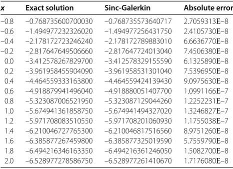
Table 4 The numerical results for the approximate solutions obtained by sinc-Galerkin in comparison with the exact solutions of Eq. (4.3) forN= 100
x Exact solution Sinc-Galerkin Absolute error
–0.8 –0.768735600700030 –0.768735573640717 2.7059313E–8 –0.6 –1.494977232326020 –1.494977256431750 2.4105730E–8 –0.4 –2.178172723246240 –2.178172789883010 6.6636770E–8 –0.2 –2.817647649506660 –2.817647724013040 7.4506380E–8 0.0 –3.412578267829700 –3.412578329155590 6.1325890E–8 0.2 –3.961958455904090 –3.961958531301040 7.5396950E–8 0.4 –4.464559333163800 –4.464559424139430 9.0975630E–8 0.6 –4.918879941496040 –4.918880051407700 1.0991166E–7 0.8 –5.323087006521950 –5.323087129044260 1.2252231E–7 1.0 –5.674941361858750 –5.674941494327020 1.3246827E–7 1.2 –5.971708083510550 –5.971708201060930 1.1755038E–7 1.4 –6.210046727765300 –6.210046817516560 8.9751260E–8 1.6 –6.385877267459800 –6.385877325019590 5.7559790E–8 1.8 –6.494216346163350 –6.494216361246050 1.5082700E–8 2.0 –6.528977278586750 –6.528977261410670 1.7176080E–8
The exact solution of (.) is
y(x) = ,, ,,x+
, ,,x
+ ,
,,x
– ,
, ,x
+ , ,,x
+
,x
+
x
.
We choose the weight function according to [],φ(x) =ln(–x),w(x) = φ(x), and by taking
d=π/,h=√ N,xk=
ekh
+ekh forN= , , , , the solutions in Figure and Table are
achieved.
Example . Let us have the following form of a singular Dirichlet-type boundary value
problem on the interval [, ]:
d
dxy(x) –
x
d dxy(x) +
y(x) x(x+ )= –x
,
y() = , y() = .
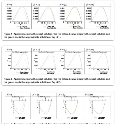
Figure 5 Approximation to the exact solution: the red colored curve displays the exact solution and the green one is the approximate solution of Eq. (4.1).
Figure 6 Approximation to the exact solution: the red colored curve displays the exact solution and the green one is the approximate solution of Eq. (4.2).
Figure 7 Approximation to the exact solution: the red colored curve displays the exact solution and the green one is the approximate solution of Eq. (4.3).
The problem has an exact solution like
y(x) = ·
ln(x+ )x+ ln(x+ ) – x+ x– xln()
– x+ xln() +x– xln() + x– xln()/– + ln(), whereφ(x) =ln(
–x),w(x) =
φ(x). By takingd=π/,h= √
N,xk= ekh
+ekhforN= , , , ,
we get the solutions in Figure and Table .
Example . The following problem is given on the interval [–, ]:
d
dxy(x) –
d
dxy(x) = –(x– ), y(–) = , y() = ,
(.)
where the exact solution of (.) isy(x) =xe–xe–+ex–xe+xe––e–e–
In this case,φ(x) =ln(–x+x),w(x) =φ(x), and by takingd=π/,h=√N,xk=–+e
kh
+ekh for
N= , , , , we get results in Figure and Table .
5 Conclusion
The sinc-Galerkin method was employed to find the solutions of second-order Dirichlet-type boundary value problems on some closed real interval. The main purpose was to find the solution of boundary value problems which arise from the singular problems. The ex-amples show that the accuracy improves with increasing number of sinc grid pointsN. We have also developed a very efficient and rapid algorithm to solve second-order Dirichlet-type BVPs with the sinc-Galerkin method on the Maple computer algebra system. All of the above computations and graphical representations were prepared by using Maple.
We give the Maple code in the Appendix section.
Appendix: Maple code which we developed for the sinc-Galerkin approximation
> restart: > with(linalg):
> with(LinearAlgebra):
> N:=:
> P(x):=-();
P(x) := –
> Q(x):=;
Q(x) :=
> F(x):=-(x-);
F(x) := –x+
> Boundaries:=z(-)=,z()=;
Boundaries :=z(–) = , z() =
> Example:=diff(z(x),x$)+P(x)*diff(z(x),x$)+Q(x)*z(x)=F(x);
Example :=
d
dxz(x)
–
d dxz(x)
= –x+
> Exact_sol:=unapply(simplify(rhs(dsolve({Example,Boundaries},z(x)))),x);
Exact_sol :=x→
xe–xe(–)+ ex– xe+ xe(–)– e– e(–) e–e(–)
> delta[]:=unapply(piecewise(j=k,,j<>k,((-)^(k-j))/(k-j)),j,k):
> delta[]:=unapply(piecewise(j=k,(-Pi^)/,j<>k,-*(-)^(k-j)/(k-j)^),j,k):
> d:=Pi/: > h:=/sqrt(N):
> xk:=unapply((-+*exp(k*h))/(+exp(k*h)),k);
xk:=k→– + e
(/k)
+e(/k)
> phi:=unapply(log((x+)/(-x)),x);
φ:=x→ln
x+ –x+
> Dphi:=unapply(simplify(diff(phi(x),x)),x): > Dphi:=unapply(simplify(diff(phi(x),x$)),x):
> g:=unapply(/Dphi(x),x):
> Dg:=unapply(simplify(diff(g(x),x$)),x): > Dg:=unapply(simplify(diff(g(x),x$)),x):
> sys:=[]:
> for p from -N to N do
sys:=[op(sys), h*(sum(y[j]*((/h^)*delta[](p,j)*
(Dphi(xk(j))*g(xk(j)))+ (/h^)*delta[](p,j)* ((Dphi(xk(j))/Dphi(xk(j)))* g(xk(j))+*Dg(xk(j)))+
(/h^)*delta[](p,j)* ((Dg(xk(j))/Dphi(xk(j))))), j=-N..N)
-sum(y[j]*((/h^)*delta[](p,j)* (subs(x=xk(j),P(x)*g(x)))+ (/h^)*delta[](p,j)*
(subs(x=xk(j),diff(P(x)*g(x),x)))/Dphi(xk(j)) ),j=-N..N)
+y[p]*subs(x=xk(p),g(x)*Q(x))/Dphi(xk(p)) -subs(x=xk(p),g(x)*F(x))/Dphi(xk(p)))=]: od:
> evalf(sys):
> A,b:=LinearAlgebra[GenerateMatrix](evalf(sys),[vars]):
> c:=linsolve(A,b):
>
ApproximateSol:=unapply(sum(c[j+N+]*sin(Pi*(phi(x)-j*h)/h)/(Pi*(phi(x)-j*h)/h),j=-N..N),x):
> plot([Exact_sol(x),ApproximateSol(x)],x=-.., title ="Sinc-Galerkin Approximation",labels=["x","y"], legend = ["Exact Solution","Sinc-Galerkin"],);
> Digits := ;
Digits :=
> Exact:=[]:Apprx:=[]:Err:=[]:
for s from -. by . to do
Exact:=[op(Exact),evalf(Exact_sol(s))]:
Apprx:=[op(Apprx),evalf(ApproximateSol(s))]: Err:=[op(Err),evalf(abs(evalf(ApproximateSol(s))-evalf(Exact_sol(s))))]:
od:
> latex(Exact);latex(Apprx);latex(Err);
[–., –., –.,
– ., –., –.,
– ., –., –.,
– ., –., –.,
– ., –., –.]
[–., –., –.,
– ., –., –.,
– ., –., –.,
– ., –., –.,
– ., –., –.]
[., ., .,
., ., .,
., ., .,
., ., .,
Competing interests
The authors declare that they have no competing interests.
Authors’ contributions
AS proposed main idea of the solution schema by using Sinc Method for linear BVPs. He developed computer algorithm and worked on theoretical aspect of problem. MK searched the materials about study and compared with other techniques, contributed with his experience on Nonlinear Approximation methods.
Author details
1Department of Mathematical Engineering, Faculty of Chemical and Metallurgical Engineering, Yildiz Technical University,
Davutpasa, ˙Istanbul, 34210, Turkey. 2Department of Mathematics, Faculty of Art and Sciences, Yildiz Technical University,
Davutpasa, ˙Istanbul, 34210, Turkey.
Received: 22 September 2012 Accepted: 15 October 2012 Published: 29 October 2012 References
1. Stenger, F: Approximations via Whittaker’s cardinal function. J. Approx. Theory17, 222-240 (1976)
2. Stenger, F: A sinc-Galerkin method of solution of boundary value problems. Math. Comput.33, 85-109 (1979) 3. Whittaker, ET: On the functions which are represented by the expansions of the interpolation theory. Proc. R. Soc.
Edinb.35, 181-194 (1915)
4. Whittaker, JM: Interpolation Function Theory. Cambridge Tracts in Mathematics and Mathematical Physics, vol. 33. Cambridge University Press, London (1935).
5. Lund, J: Symmetrization of the sinc-Galerkin method for boundary value problems. Math. Comput.47, 571-588 (1986)
6. Lund, J, Bowers, KL: Sinc Methods for Quadrature and Differential Equations. SIAM, Philadelphia (1992)
7. Lewis, DL, Lund, J, Bowers, KL: The space-time sinc-Galerkin method for parabolic problems. Int. J. Numer. Methods Eng.24, 1629-1644 (1987)
8. McArthur, KM, Bowers, KL, Lund, J: Numerical implementation of the sinc-Galerkin method for second-order hyperbolic equations. Numer. Methods Partial Differ. Equ.3, 169-185 (1987)
9. Bowers, KL, Lund, J: Numerical solution of singular Poisson problems via the sinc-Galerkin method. SIAM J. Numer. Anal.24(1), 36-51 (1987)
10. Lund, J, Bowers, KL, McArthur, KM: Symmetrization of the sinc-Galerkin method with block techniques for elliptic equations. IMA J. Numer. Anal.9, 29-46 (1989)
11. Lybeck, NJ: Sinc domain decomposition methods for elliptic problems. PhD thesis, Montana State University, Bozeman, Montana (1994)
12. Lybeck, NJ, Bowers, KL: Domain decomposition in conjunction with sinc methods for Poisson’s equation. Numer. Methods Partial Differ. Equ.12, 461-487 (1996)
13. Morlet, AC, Lybeck, NJ, Bowers, KL: The Schwarz alternating sinc domain decomposition method. Appl. Numer. Math.
25, 461-483 (1997)
14. Morlet, AC, Lybeck, NJ, Bowers, KL: Convergence of the sinc overlapping domain decomposition method. Appl. Math. Comput.98, 209-227 (1999)
15. Alonso, N, Bowers, KL: An alternating-direction sinc-Galerkin method for elliptic problems. J. Complex.25, 237-252 (2009)
16. Ng, M: Fast iterative methods for symmetric sinc-Galerkin systems. IMA J. Numer. Anal.19, 357-373 (1999)
17. Ng, M, Bai, Z: A hybrid preconditioner of banded matrix approximation and alternating-direction implicit iteration for symmetric sinc-Galerkin linear systems. Linear Algebra Appl.366, 317-335 (2003)
18. Stenger, F: Numerical Methods Based on Sinc and Analytic Functions. Springer, New York (1993)
19. Koonprasert, S: The sinc-Galerkin method for problems in oceanography. PhD thesis, Montana State University, Bozeman, Montana (2003)
20. McArthur, KM, Bowers, KL, Lund, J: The sinc method in multiple space dimensions: model problems. Numer. Math.56, 789-816 (1990)
21. Stenger, F: Numerical methods based on Whittaker cardinal, or sinc functions. SIAM Rev.23, 165-224 (1981) 22. Stenger, F: Summary of sinc numerical methods. J. Comput. Appl. Math.121, 379-420 (2000)
23. Stenger, F, O’Reilly, MJ: Computing solutions to medical problems via sinc convolution. IEEE Trans. Autom. Control43, 843 (1998)
24. Narasimhan, S, Majdalani, J, Stenger, F: A first step in applying the sinc collocation method to the nonlinear Navier Stokes equations. Numer. Heat Transf., Part B41, 447-462 (2002)
25. Mueller, JL, Shores, TS: A new sinc-Galerkin method for convection-diffusion equations with mixed boundary conditions. Comput. Math. Appl.47, 803-822 (2004)
26. El-Gamel, M, Behiry, SH, Hashish, H: Numerical method for the solution of special nonlinear fourth-order boundary value problems. Appl. Math. Comput.145, 717-734 (2003)
27. Lybeck, NJ, Bowers, KL: Sinc methods for domain decomposition. Appl. Math. Comput.75, 4-13 (1996) doi:10.1186/1687-2770-2012-126