www.geosci-model-dev.net/5/269/2012/ doi:10.5194/gmd-5-269-2012
© Author(s) 2012. CC Attribution 3.0 License.
Geoscientific
Model Development
The FAMOUS climate model (versions XFXWB and XFHCC):
description update to version XDBUA
R. S. Smith
NCAS-Climate, Dept. of Meteorology, University of Reading, UK
Correspondence to: R. S. Smith ([email protected])
Received: 3 November 2011 – Published in Geosci. Model Dev. Discuss.: 22 November 2011 Revised: 15 February 2012 – Accepted: 17 February 2012 – Published: 24 February 2012
Abstract. FAMOUS is an ocean-atmosphere general circu-lation model of low resolution, based on version 4.5 of the UK MetOffice Unified Model. Here we update the model description to account for changes in the model as it is used in the CMIP5 EMIC model intercomparison project (EMICmip) and a number of other studies. Most of these changes correct errors found in the code. The EMICmip ver-sion of the model (XFXWB) has a better-conserved water budget and additional cooling in some high latitude areas, but otherwise has a similar climatology to previous versions of FAMOUS. A variant of XFXWB is also described, with changes to the dynamics at the top of the model which im-prove the model climatology (XFHCC).
1 Introduction
FAMOUS (FAst Met Office/UK Universities Simulator) is an Earth System Model (ESM) derived from the Hadley Centre coupled model version 3 (HadCM3) (Gordon et al., 2000), a configuration of the UK Met Office Unified Model. Using approximately half the spatial resolution of HadCM3 and a tenth of its computational resources, FAMOUS can currently simulate∼250 yr in a day on 8 cores of a multi-core system, making GCM-complexity millennial-scale transient runs and large ensembles feasible. FAMOUS has been systematically tuned to reproduce both the equilibrium climate and climate sensitivity of HadCM3 (Jones et al. 2005; Smith et al. 2008, SOG08 hereafter).
Versions of FAMOUS are denoted by their Unified Model job codes – the version in Jones et al. (2005) was ADTAN, and SOG08 described version XDBUA. Following the pub-lication of SOG08, use of the model highlighted a system-atic instability under certain climate forcings, and a
num-ber of errors were found in the model code. These is-sues have been addressed, and here we describe the result-ing version XFXWB, which was used in Smith and Gregory (2012) and contributed to the EMICmip (www.climate.uvic. ca/EMICAR5) model intercomparison project. We also de-scribe version XFHCC, a variant of XFXWB with a different solution to the instability problems seen in XDBUA. We up-date the model description given in SOG08, outlining only the changes to the model code and climatology. This update paper assumes familiarity with the material in SOG08; the basic material therein will not be repeated.
2 Technical changes
2.1 Stratospheric winds
The vertical resolution of the atmosphere model in FAMOUS is largely responsible for biasses in both heating and winds around and above the poorly-resolved tropopause (see e.g. Fig. 5 in SOG08). In particular, the top-level winds in XD-BUA are unrealistically fast, and have been found to be the root cause of instability problems; simulations of glacial cli-mates with XDBUA have been found to be particularly un-stable (Gregoire et al., 2011).
A scientifically more satisfactory solution involves intro-ducing friction to the top levels of the model to slow the winds to more realistic speeds. This is the approach taken in XFHCC. It seems likely that the low resolution of FAMOUS prevents the gravity wave drag parameterisation from work-ing as it does in HadCM3, so another mechanism is required to remove energy from the top-level flow. Simple Rayleigh friction is added to the top three levels of the model, with timescales of (descending from the model top) 15, 30 and 60 days, respectively. These values were taken from those used in the IGCM (Forster et al., 2000), an intermediate com-plexity model of similar resolution that employs this param-eterisation, and found to produce good results. The simple cap on top-level wind speeds is not required in FAMOUS if this frictional parameterisation is used in the model.
The introduction of top-level friction to the model also removes the instability problem from XFHCC, but it also changes the surface climate significantly (see Sect. 3.2). The atmosphere in the Unified Model is a grid-point model, with Fourier filtering routines to smooth small-scale vari-ability that the grid is unable to represent. The unrealisti-cally fast top-level winds of previous versions of FAMOUS led to the over-use of these filtering routines throughout the model, damping mid-latitude variability and atmospheric en-ergy transport in the control climate. Furthermore, it appears that changes in the extreme top-level winds dominate the dy-namical response to CO2-forced climate change in previous versions of FAMOUS, producing changes in wind patterns at odds with those found in the majority of climate models. Introducing friction in the top-level of FAMOUS thus has di-rect effects throughout the model. To take best practical ad-vantage of this new parameterisation would require retuning other parameters in the model – ozone, and sea-ice albedo, for instance (see SOG08). This retuning is being done in con-junction with other major changes to the land surface model in FAMOUS, and will be described in a forthcoming paper. In the second half of this paper, the physical impact of the introduction of top-level friction alone will be described.
2.2 Snow overlying coastal sea-ice
One of the primary differences between FAMOUS and its parent model HadCM3 is the use of coastal tiling in FA-MOUS. This mitigates the impact of FAMOUS’s lower reso-lution on the land-sea interface by allowing coastal gridboxes in the atmosphere to see boundary conditions for land and sea simultaneously. The land model in XDBUA, however, only contained one snow-depth field. This meant that, during the ocean-atmosphere coupling step, snow lying in the land frac-tion of coastal gridboxes was overwritten by the field from the ocean fraction which held snow lying on sea-ice. Land-based coastal snow was thus lost from the model at the end of every day, resulting in not only a non-conservation of wa-ter in the model but also erroneous temperature and albedo effects.
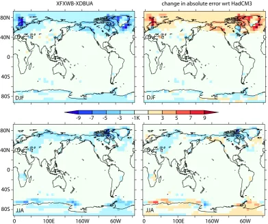
A separate prognostic field for sea-ice based snow has now been implemented. The primary effect of this has been to cool coastal regions of the model during winter: the majority of the change apparent in Fig. 1 is due to the correction of this error.
2.3 Ocean sensible/latent heat fluxes
During the calculation of surface turbulence over the ocean, the gridbox-mean sensible and latent heat fluxes are erro-neously interchanged. The impact of this error appears to be limited to boundary layer stability calculations that affect convection in the model, as the gridbox-means are calculated anew in the next subroutine. The resolution of this error does not appear to have had a significant impact on the preindus-trial control climate of FAMOUS.
2.4 Ocean penetration of solar radiation
FAMOUS contains a version of the ocean biogeochemistry model HadOCC (Palmer and Totterdell, 2001), which some users choose to disable for reasons of computational effi-ciency. The version of HadOCC used in FAMOUS con-tains routines for altering the sub-surface penetration of so-lar radiation in the ocean according to plankton levels. In XDBUA, the code was written such that simply disabling HadOCC through FAMOUS’s user interface left these rou-tines in place, with the resulting modifications of solar pen-etration becoming undefined. Correcting this error has not been shown to produce significant effects in the climate of FAMOUS, but its impact is compiler and runtime dependent so is difficult to assess.
2.5 Minor issues
The version of HadOCC in XDBUA contained an undocu-mented code change, whereby the diagnostic of zooplankton production in fact shows calcite export instead. This has now been corrected. Code for the third-order advection scheme for the biogeochemical tracers in HadOCC also clashes with the diagnostics of vertical velocity within the ocean, such that detailed energy budgets calculated from the model diagnos-tics no longer close. This issue has not yet been fixed, al-though the diagnostic of ocean temperature tendencies due to advection have been made more accurate.
In addition, FAMOUS now contains a number of minor ocean code rewrites, designed to ensure consistent code be-haviour across different compilers. The inclusion of this code has not been shown to affect the climate of FAMOUS.
3 Climatologies
-9 -7 -5 -3 -1K 1 3 5 7 9
JJA DJF
JJA DJF
XFXWB-XDBUA change in absolute error wrt HadCM3
80N
40N
0
40S
80S
80N
40N
0
40S
80S
0 100E 160W 60W 0 100E 160W 60W
Fig. 1. Difference in seasonal surface temperature. Left: XFXWB-XDBUA; right: change in magnitude of error with respect to HadCM3; top: DJF; below: JJA.
3.1 XFXWB climatology
A series of standard experiments were conducted with XFXWB, including a preindustrial control run and a num-ber of idealised CO2forcing experiments. These have been submitted to the EMICmip model intercomparison project (www.climate.uvic.ca/EMICAR5). The setup of the prein-dustrial control run of XFXWB differs from that of XD-BUA in a number of ways. XDXD-BUA used a somewhat ad-hoc collection of “modern” boundary conditions, with an at-mosphericpCO2of 290 ppmv but orbital parameters appro-priate for 2000 CE. XFXWB, rather more consistently, uses an atmosphericpCO2of 282 ppmv, and orbital parameters from 1850 CE. The value of the solar constant is also slightly different, consistent with historical records. The imposed iceberg calving field (see SOG08 for details) has also been slightly recalibrated for this run to better conserve global ocean salinity. XFXWB was run on 5000 yr from the end of the 6000 yr control run of XDBUA. At the end of the spinup, all surface fields in XFXWB are in equilibrium, with a drift of 0.003◦C century−1in bottom ocean temperatures, and a drift in global average salinity of−2.34×10⁻⁶psu yr−1.
The main difference between XDBUA and XFXWB lies in the surface temperatures (Fig. 1, left). This is mostly driven by the increase in coastal snow cover that results from the fix described in Sect. 2.2. Expressed as radiative forcings, the changes in solar and greenhouse gas boundary condi-tions noted above would be expected to result in a global, annual average cooling of around 0.1◦C, although the sea-sonal changes in orbital forcing might, in fact, be expected to produce a net warming of around 1◦C over high latitudes in
winter and spring. Compared to XDBUA, XFXWB has cool-ing in December, January and February (DJF) of up to 2◦C
on Antarctica and in the Arctic, with additional patches of en-hanced cooling around the coasts, especially in the North Pa-cific. In June, July and August (JJA) there is a small cooling over the Northern Hemisphere land masses. There are small (generally<0.1) increases in annual mean sea-ice fraction resulting from the high latitude cooling.
-18 -14 -10 -6 -2K 2 6 10 14 18
JJA DJF
JJA DJF XFXWB-NCEP
80N
40N
0
40S
80S
80N
40N
0
40S
80S
0 100E 160W 60W 0 100E 160W 60W XFHCC-NCEP
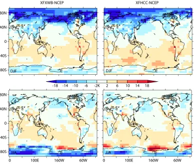
Fig. 2. Errors in seasonal surface temperature with respect to the NCEP reanalysis (Kalnay et al., 1996). Left: XFXWB-NCEP;
right: XFHCC-NCEP; top: DJF; below: JJA.
over Antarctica in DJF and the Northern Hemisphere in JJA the cooling in XFXWB tends to reduce the error. The Arcsin-Mielke skill scores with respect to HadCM3 (a metric of how well both the magnitude and pattern of two different fields match, see Jones et al. (2005) for details) for the northern high latitude (poleward of 45◦N) surface temperature pat-terns which dominate the bias in FAMOUS are correspond-ingly a little lower for XFXWB than XDBUA in DJF and the annual mean, although still higher than in ADTAN, the origi-nal version of FAMOUS (Table 1). FAMOUS’s most notable problem remains a high latitude winter cold bias (Fig. 2, left), compounded by an over-estimate of winter sea-ice coverage in the Northern Hemisphere.
In experiments with elevated levels of atmosphericpCO2 (not shown), XFXWB has been found to display a slow long-term surface temperature drift (around 0.2◦C per century).
This makes defining a single number for its climate sen-sitivity hard, but taken over the first 150 yr of more rapid adjustment to an instantaneous increase to four times pre-industrial atmospheric CO2, XFXWB has a slightly lower climate feedback parameter (Gregory et al., 2004) than XD-BUA of 0.91±0.05 W m−2K−1, closer to the value of AD-TAN than HadCM3.
Table 1. Arcsin-Mielke skill scores for surface temperature
pole-ward of 45◦N with respect to HadCM3 in different versions of
FA-MOUS. Potential scores range from 1 to−1, with 1 denoting a
per-fect match between fields, 0 implying no correlation at all and−1
perfect anti-correlation.
ADTAN XDBUA XFXWB XFHCC
DJF 0.60 0.70 0.63 0.79
JJA 0.79 0.76 0.80 0.84
Annual 0.66 0.77 0.72 0.85
3.2 XFHCC climatology
80S 40S 0 40N 80N
200
400
600 mbar 800
1000
40 30 20 10 0 m/s -10 -20 -30 -40
XFHCC
40 30 20 10 0 m/s -10 -20 -30 -40
HadCM3
200
400
600 mbar 800
1000
200
400
600 mbar 800
1000 XDBUA
40 30 20 10 0 m/s -10 -20 -30 -40
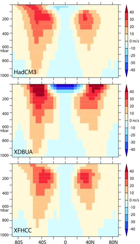
Fig. 3. Annual, zonal average zonal winds. Top: HadCM3; mid-dle: XDBUA; bottom: XFHCC.
XFXWB, and run for 1000 yr. Rather than providing a new control climate for FAMOUS, this experiment is designed to show the impact of the top-level friction alone. A fully re-tuned version of the model, combining the top-level friction with a number of other major changes to the science in FA-MOUS, will be described in a forthcoming paper.
This brings the vertical distribution of zonal winds into much better agreement with both observations and higher resolution models (Fig. 3). The vertical temperature profile in the model is also improved, following the thermal wind relation.
The immediate effect of the introduction of top-level fric-tion in FAMOUS is the improvement in the general shape of the zonal winds in XFHCC (Fig. 3). Maxima in the jets move to their correct location and magnitude at around 30 m s−1
80S 40S 0 40N 80N 50
40
30
20
10
0
HadCM3 (HadCM3)/2
XDBUA XFHCC
w
av
enumb
er
Fig. 4. Maximum wavenumber allowed by the Fourier filtering in DJF. Black, solid: HadCM3; black, dashed: HadCM3 data divided by 2, a profile that might be expected of a model with half the reso-lution of HadCM3; green: XDBUA; blue: XFHCC.
at 200 mbar, rather than increasing to ±70 m s−1 or more in the top level of the model. Vertical temperature profiles at higher latitudes now suggest a more realistic tropopause height (see Fig. 5, SOG08) and imply that more realistic lev-els of ozone than the low values specified in XDBUA could now be used to improve stratospheric temperature profiles. The reduction in strength of the jets however reduces their vertical extent as well, leading to weaker zonal winds at the surface in XFHCC. The most immediate impact of this is a reduction in the strength of the Antarctic Circumpolar Cur-rent (ACC), from around 70 Sv to around 50 Sv, which is at the lower end of the range of values in the coupled model intercomparison database of Meehl et al. (2007).
The slowing in top-level winds reduces the impact of the Fourier filtering routines in the model that are intended to re-move subgridscale variability at high latitudes. These rou-tines are clearly over-active in XDBUA, cutting out fea-tures with wavenumbers above 6 poleward of 50◦N in DJF (Fig. 4). By contrast, filtering in XFHCC follows a profile more in line with that expected for a model with FAMOUS’s resolution, allowing wavenumbers up to around 15 at 50◦N in DJF.
-9 -7 -5 -3 -1K 1 3 5 7 9
XFHCC-XFXWB change in absolute error wrt HadCM3
DJF
JJA
DJF
JJA 80N
40N
0
40S
80S
80N
40N
0
40S
80S
0 100E 160W 60W 0 100E 160W 60W
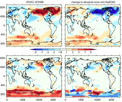
Fig. 5. Difference in seasonal surface temperature. Left: XFHCC-XFXWB; right: change in magnitude of error with respect to HadCM3; top: DJF; below: JJA.
90S 60S 30S 0 30N 60N 90N 0.6
0.4
0.2
0 PW
-0.2
-0.4
-0.6
XDBUA-HadCM3 XFHCC-HadCM3
Fig. 6. Difference in magnitude of the annual average
at-mospheric energy transport between FAMOUS and HadCM3. Black: XDBUA-HadCM3; red: XFHCC-HadCM3.
from an anomalous cyclonic circulation which brings Arc-tic air down over eastern Europe, with a local surface albedo effect due to enhanced snow cover.
XFHCC
4.5 3.5 2.5 1.5 0.5 m/s -0.5 -1.5 -2.5 -3.5 -4.5
80S 40S 0 40N 80N 200
400
600 mbar
800
1000 XFXWB
4.5 3.5 2.5 1.5 0.5 m/s -0.5 -1.5 -2.5 -3.5 -4.5 200
400
600 mbar
800
1000
HadCM3
4.5 3.5 2.5 1.5 0.5m/s -0.5 -1.5 -2.5 -3.5 -4.5 200
400
600 mbar
800
1000
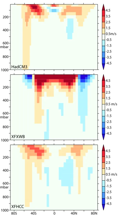
Fig. 7. Changes in annual average, zonal average winds at 2×CO2
in 1 % CO2increase runs. Top: HadCM3; middle: XFXWB;
bot-tom: XFHCC.
The Atlantic meridional overturning circulation also changes between XFXWB and XFHCC, with both the max-imum and the overall shape of the overturning becoming significantly deeper, extending to the bottom and exclud-ing Antarctic bottom water (AABW) from the Atlantic in XFXWB. It is not clear whether this results from the changes in surface temperature and ice coverage in the North Atlantic, a response to the weaker ACC (and likely weaker AABW formation, which is well correlated with the strength of the ACC; Gent et al., 2001), or some combination of these and other climate feedbacks.
Simulations with elevated levels of atmospheric CO2have also been conducted with XFHCC. These do not appear to show the same long-term drift as in XFXWB, and are slightly less sensitive, with a climate feedback parameter that is much
the same as XDBUA, at 1.10±0.05 W m−2K−1. Changes in the precipitation fields under CO2 forcing are very sim-ilar in XFXWB and XFHCC. In such climate simulations, most models show a southward shift and intensification of Southern Ocean westerly winds (Wang et al., 2011). To com-pare with HadCM3 data, atmospheric CO2in FAMOUS was increased at 1 % a year until twice the pre-industrial value of CO2was reached. In this experiment, XFXWB shows a weakening of the winds over the Southern Ocean. XFHCC does produce some intensification of Southern Ocean west-erlies under this atmospheric CO2 forcing, which can be clearly traced back to the response of the high-altitude winds (Fig. 7), which is no longer dominated by the unrealistically high winds in the top level of XFXWB.
4 Summary and outlook
Changes to the formulation of FAMOUS since version XD-BUA have been described. Despite a number of non-trivial technical improvements to the code, version XFXWB has a climatology that differs little from XDBUA, the main changes being a coastal cooling at high latitudes and a sig-nificant increase in model stability. Version XFHCC con-tains an additional improvement to the parameterisation of high-altitude winds that leads to a model climatology that is much improved in several other respects. NetCDF files of climatological data for the control simulations of XFXWB and XFHCC are provided in the supplementary material to this article.
All currently described versions of FAMOUS (ADTAN, XDBUA, XFXWB and XFHCC) employ the MOSES1 land surface scheme (Cox et al., 1999) as used in HadCM3. A new version of FAMOUS, containing the MOSES2.2 scheme (Essery et al., 2003), is currently being tuned. This ver-sion is capable of a simple closed carbon cycle and dynamic vegetation, as well as containing all the improvements de-scribed here and a more realistic sea-ice model, and will be described in a forthcoming publication. This new ver-sion of FAMOUS is also under further development to al-low for subgridscale coupling of MOSES2.2 to the Glim-mer community ice-sheet model, improving on the simple annual positive-degree-day coupling currently used for ice-sheet mass balance in Glimmer. More information on the use and development of FAMOUS can be found on the website at http://www.famous.ac.uk.
Supplementary material related to this article is available online at:
Acknowledgements. I would like to acknowledge the support of
Annette Osprey, Simon Wilson and other members of the NCAS Computer Modelling Support team in support of FAMOUS. Discussions with the community of FAMOUS users, notably
Jonathan Gregory1,2 and Manoj Joshi1 of NCAS-Climate1 and
the UK Met Office2, and members of the BRIDGE group in the
Geography Department of the University of Bristol, contribute
greatly to the ongoing development of the model. XFXWB
was integrated on HECToR, the UK National Supercomputing
resource. We would also like to thank Chris Jones2 and the
UK Met Office for the original Unified Model code used in
FAMOUS, and Hugo Lambert2, who contributed improvements
to the ocean code. NCEP Reanalysis data provided by the
NOAA/OAR/ESRL PSD, Boulder, Colorado, USA, from their Web
site at http://www.esrl.noaa.gov/psd. This paper was improved
thanks to comments by Chris Jones and an anonymous reviewer.
Edited by: D. Lunt
References
Cox, P. M., Betts, R. A., Bunton, C. B., Essery, R. L. H., Rowntree, P. R., and Smith, J.: The impact of new land surface physics on the GCM simulation of climate and climate sensitivity, Clim. Dynam., 15, 183–203, 1999.
Essery, R. L. H., Best, M. J., Betts, R. A., Cox, P. M., and Taylor, C. M.: Explicit representation of subgrid heterogeneity in a GCM land-surface scheme, J. Hydrometeorol., 4, 530–543, 2003. Forster, P. d. F., Blackburn, M., Glover, R., and Shine, K.: An
examination of climate sensitivity for idealised climate change experiments in an intermediate general circulation model, Clim. Dynam., 16, 833–849, 2000.
Gent, P., Large, W., and Bryan, F.: What sets the mean transport through the Drake Passage?, J. Geophys. Res., 106, 2693–2712, 2001.
Gordon, C., Cooper, C., Senior, C. A., Banks, H., Gregory, J. M., Johns, T. C., Mitchell, J. F. B., and Wood, R. A.: The simulation of SST, sea ice extents and ocean heat transports in a version of the Hadley Centre coupled model without flux adjustments, Clim. Dynam., 16, 147–168, 2000.
Gregoire, L. J., Valdes, J. P., Payne, A. J., and Kahana, R.: Optimal tuning of a GCM using modern and glacial constraints, Clim. Dynam., 37, 705–719, 2011.
Gregory, J. M., Ingram, W. J., Palmer, M. A., Jones, G. S., Stott, P. A., Thorpe, R. B., Lowe, J. A., Johns, T. C., and Williams, K. D.: A new method for diagnosing radiative forc-ing and climate sensitivity, Geophys. Res. Lett., 31, L03205, doi:10.1029/2003gl018747, 2004.
Jones, C., Gregory, J., Thorpe, R., Cox, P., Murphy, J., Sexton, D., and Valdes, P.: Systematic optimisation and climate simulations of FAMOUS, a fast version of HadCM3, Clim. Dynam., 25, 189– 204, 2005.
Kalnay, E., Kanamitsu, M., Kistler, R., Collins, W., Deaven, D., Gandin, L., Iredell, M., Saha, S., White, G., Woollen, J., Zhu, Y., Chelliah, M., Ebisuzaki, W., Higgins, W., Janowiak, J., Mo, K. C., Ropelewski, C., Wang, J., Leetmaa, A., Reynolds, R., Jenne, R., and Joseph, D.: The NCEP/NCAR 40-Year Reanal-ysis Project, Bull. Am. Meteorol. Soc., 77, 437–471, 1996. Meehl, G. A., Covey, C., Delworth, T., Latif, M., McAveney, B.,
Mitchell, J. F. B., Stouffer, R. J., and Taylor, K. E.: The WCRP CMIP3 multi-model dataset: A new era in climate change re-search, Bull. Am. Meteorol. Soc., 88, 1383–1394, 2007. Palmer, J. R. and Totterdell, I. J.: Production and export in a global
ocean ecosystem model, Deep-Sea Res. I, 48, 1169–1198, 2001.
Smith, R. S. and Gregory, J. M.: The last glacial cycle:
transient simulations with an AOGCM, in press, Clim. Dy-nam., doi:10.1007/s00382-011-1283-y, www.springerlink.com/ content/a3244p375452q180, 2012.
Smith, R. S., Gregory, J. M., and Osprey, A.: A description of the FAMOUS (version XDBUA) climate model and control run, Geosci. Model Dev., 1, 53–68, doi:10.5194/gmd-1-53-2008, 2008.