Forward-Backward Selection with Early Dropping

(1)

Forward-Backward Selection with Early Dropping

Computer Science Department, University of Crete Gnosis Data Analysis

Editor:Isabelle Guyon

Abstract

Forward-backward selection is one of the most basic and commonly-used feature selection algorithms available. It is also general and conceptually applicable to many different types of data. In this paper, we propose a heuristic that significantly improves its running time, while preserving predictive performance. The idea is to temporarily discard the variables that are conditionally independent with the outcome given the selected variable set. De-pending on how those variables are reconsidered and reintroduced, this heuristic gives rise to a family of algorithms with increasingly stronger theoretical guarantees. In distribu-tions that can be faithfully represented by Bayesian networks or maximal ancestral graphs, members of this algorithmic family are able to correctly identify the Markov blanket in the sample limit. In experiments we show that the proposed heuristic increases computational efficiency by about 1-2 orders of magnitude, while selecting fewer or the same number of variables and retaining predictive performance. Furthermore, we show that the proposed algorithm and feature selection with LASSO perform similarly when restricted to select the same number of variables, making the proposed algorithm an attractive alternative for problems where no (efficient) algorithm for LASSO exists.

Keywords: Feature Selection, Forward Selection, Markov Blanket Discovery, Bayesian Networks, Maximal Ancestral Graphs

1. Introduction

The problem of feature selection (a.k.a. variable selection) in supervised learning tasks can be defined as the problem of selecting a minimal-size subset of the variables that leads to an optimal, multivariate predictive model for a target variable (outcome) of interest (Tsamardinos and Aliferis, 2003). Thus, the feature selection’s task is to filter out irrelevant variables and variables that are superfluous given the selected ones (that is, weakly relevant variables, see (John et al., 1994; Tsamardinos and Aliferis, 2003)).

Solving the feature selection problem has several advantages. Arguably, the most impor-tant one is knowledge discovery: by removing superfluous variables it improves intuition and understanding about the data-generating mechanisms. This is no accident as solving the feature selection problem has been linked to the data-generating causal network (Tsamardi-nos and Aliferis, 2003). In fact,it is often the case that the primary goal of data analysis is feature selection and not the actual resulting predictive model. This is particularly true in medicine and biology where the features selected may direct future experiments and studies. Feature selection is also employed to reduce the cost of measuring the features to make

op-c

(2)

erational a predictive model; for example, it can reduce the monetary cost or inconvenience to a patient of applying a diagnostic model by reducing the number of medical tests and measurements required to perform on a subject for providing a diagnosis. Feature selection also often improves the predictive performance of the resulting model in practice, especially in high-dimensional settings. This is because a good-quality selection of features facilitates modeling, particularly for algorithms susceptible to the curse of dimensionality. There has been a lot of research on feature selection methods in the statistical and machine learning literature. An introduction to the topic, as well as a review of many, prominent methods can be found in (Guyon and Elisseeff, 2003), while the connections between feature selec-tion, the concept of relevancy, and probabilistic graphical models is in (John et al., 1994; Tsamardinos and Aliferis, 2003).

We will focus on forward and backward selection algorithms, which are specific instances of stepwise methods (Kutner et al., 2004; Weisberg, 2005). These methods are some of the oldest, simplest and most commonly employed feature selection methods. An attractive property of stepwise methods is that they are very general, and are applicable to different types of data. For instance, stepwise methods using conditional independence tests can be directly applied to (a) mixed continuous and categorical predictors, (b) cross-sectional or time course data, (c) continuous, nominal, ordinal or time-to-event outcomes, among others, (d) with non-linear tests, such as kernel-based methods (Zhang et al., 2011), and (e) to heteroscedastic data using robust tests; many of the aforementioned tests, along with others have been implemented in the MXM R package (Lagani et al., 2017). The main drawback of forward selection is its computational cost. In order to select k variables, it performs O(pk) tests for variable inclusion, where p is the total number of variables in the input data. This is acceptable for low-dimensional datasets, but becomes unmanageable with increasing dimensionality. Another issue is that forward selection suffers from multiple testing problems and thus may select a large number of irrelevant variables (Flom and Cassell, 2007).

(3)

the most additional information, given all selected variables. In LASSO, both forward and backward steps can be performed at each iteration. After a feature is selected, forward selection and OMP create a new unrestricted model that also contains the newly selected feature. LASSO, LARS and FSR create a new model by updating the previous one, con-straining the coefficients of the new model. LASSO has a stopping criterion based on the L1-norm of the coefficients of the current variables. Given this synthetic view and connec-tions between the algorithms, we would like to note that any extension to stepwise methods, such as the one proposed in this work, can be translated and directly applied with any of the above feature selection algorithms.

In this work we extend the forward selection algorithm to deal with the problems above. In Section 3 we proposeearly dropping, a simple heuristic to speed-up forward selection, without sacrificing its quality and maintaining its theoretical guarantees. The idea is, in each iteration of the forward search, to filter out variables that are deemed conditionally independent of the target given the current set of selected variables. After termination, the algorithm is allowed to run up toK additional times, every time initializing the set of selected variables to the ones selected in the previous run. Finally, backward selection is applied on the result of the forward phase. We call this algorithm Forward-Backward selection with Early Dropping (FBEDK)1. This heuristic is inspired by the theory of Bayesian networks and maximal ancestral graphs (Spirtes et al., 2000; Richardson and Spirtes, 2002), and similar ideas have been successfully applied for feature selection (Aliferis et al., 2010). In Section 3.2 we show that (a) FBED0 returns a superset of the adjacent nodes in any Bayesian network or maximal ancestral graph that faithfully represents the data distribution (if there exists one and assuming perfect statistical independence tests), (b) FBED1 returns the Markov blanket of the data distribution, provided the distribution is faithful to a Bayesian network, and (c) FBED∞ returns the Markov blanket of the data distribution provided the distribution is faithful to a maximal ancestral graph, or equiva-lently, it is faithful to a Bayesian network where some variables are unobserved (latent). In the experimental evaluation presented in Section 4, we show that FBEDK is 1-2 orders of magnitude faster than FBS, while at the same time selecting a similar number of features and having similar predictive performance. In a comparison between different members of the FBEDK family and FBS we show that FBED0 and FBED1 also reduce the number of false variable selections, when the data consist of irrelevant variables only. We also investi-gated the behavior of FBEDK with increasing number of runsK, showing that a relatively smallK is sufficient in most cases to reach optimal predictive performance. Afterwards, we compare FBEDK to FBS, feature selection with LASSO (Tibshirani, 1996) and to the Max-Min Parents and Children algorithm (MMPC) (Tsamardinos et al., 2003a) and show that it often has comparable predictive performance while selecting the fewest variables overall. Finally, we compare FBEDK to feature selection with LASSO (Tibshirani, 1996) when both algorithms are limited to select the same number of variables, showing that both algorithms perform similarly. This, along with the generality of FBEDK makes it an interesting alter-native to LASSO, especially for problems where LASSO requires specialized algorithms (like the group LASSO algorithm for logistic regression (Meier et al., 2008), LASSO for

(4)

effects linear models (Schelldorfer et al., 2011), and the LASSO and group LASSO methods for functional Poisson regression (Ivanoff et al., 2016)), which may be non-convex (as is the case for mixed-effects linear models (Schelldorfer et al., 2011) or for temporal-longitudinal data (Groll and Tutz, 2014; Tsagris et al., 2018)) and computationally demanding (taking several days to terminate on datasets with just 1000 predictors using Cox’s proportional hazards model (Fan et al., 2010)).

2. Notation and Preliminaries

We start by introducing the notation and terminology used throughout the paper. We use upper-case letters to denote single variables (for example, X), and bold upper-case letters to denote sets of variables (for example,Z). The terms variable, feature or predictor will be used interchangeably. We will use pand nto refer to the number of variables and samples in a dataset D, respectively. The set of variables in D will be denoted as V. The target variable (also called outcome) will be referred to as T. Next, we proceed with the basics about stepwise feature selection methods (Kutner et al., 2004; Weisberg, 2005).

2.1. Stepwise Feature Selection

Stepwise methods start with some set of selected variables and try to improve it in a greedy fashion, by either including or excluding a single variable at each step. There are various ways to combine those operations, leading to different members of the stepwise algorith-mic family. Two popular members of the stepwise family are the forward selection and

backward selection(also known as backward elimination) algorithms. Forward selection starts with a (usually empty) set of variables and adds variables to it, until some stop-ping criterion is met. Similarly, backward selection starts with a (usually complete) set of variables and then excludes variables from that set, again, until some stopping criterion is met. Typically, both methods try to include or exclude the variable that offers the highest performance increase. We will call each step of selecting (removing) a variable a forward (backward) iteration. Executing forward (backward) iterations until termination will be called a forward (backward)phase respectively. An instance of the stepwise family, which we focus on hereafter, is theForward-Backward Selectionalgorithm (FBS), which first performs a forward phase and then a backward phase on the selected variables. This algo-rithm is not new; similar algoalgo-rithms have appeared in the literature before (Margaritis and Thrun, 2000; Tsamardinos et al., 2003b; Margaritis, 2009).

FBS is shown in Algorithm 1. The functionPerfevaluates a set of variables and returns their performance relative to some statistical model. Examples are the log-likelihood for logistic regression, the partial log-likelihood for Cox regression and the F-score for linear regression, or their AIC (Akaike, 1973) or BIC (Schwarz et al., 1978) penalized variants. Theselection criterionCcompares the performance of two sets of variables as computed byPerf. For instance, in the previous exampleCcould perform a likelihood ratio test and use a predetermined significance levelαto make a decision2; we will describe such selection criteria in the next subsection. We will use the predicates>

C ,≥

C

and = C

to compare two sets

(5)

Algorithm 1 Forward-Backward Selection (FBS)

Input: Dataset D, TargetT

Output: Selected VariablesS 1: S← ∅//Set of selected variables

2: R←V //Set of remaining candidate variables

3:

4: //Forward phase: iterate until S does not change

5: while Schanges do

6: //Identify the best variableVbest out of all remaining variablesR, according to Perf 7: Vbest ← argmax

V∈R Perf

(S∪V)

8: //SelectVbest if it increases performance according to criterion C 9: if Perf(S∪Vbest)>

C Perf

(S) then 10: S ← S∪Vbest

11: R← R\Vbest 12: end if

13: end while 14:

15: //Backward phase: iterate until S does not change

16: while Schanges do

17: //Identify the worst variableVworst out of all selected variablesS, according toPerf 18: Vworst ← argmax

V∈S Perf

(S\V)

19: //Remove Vworst if it does not decrease performance according to criterion C 20: if Perf(S\Vworst)≥

C

Perf(S) then 21: S ← S\Vworst

22: end if 23: end while 24: return S

of variables; they are true if the left-hand-side value is greater, greater or equal, or equal than the right-hand-side value respectively, according to the criterion C.

2.2. Criteria for Variable Selection

Next we will briefly describe some performance functions and selection criteria that are employed in practice; for more details see (Kutner et al., 2004; Weisberg, 2005). The most common choices are statistical tests, information criteria and cross-validation. We will focus on statistical tests, as we use them in the remainder of the paper. We will also describe information criteria and contrast them to statistical tests, but will not further consider cross-validation, mainly because of its high computational cost.

2.2.1. Statistical Tests

(6)

tests) for nested models as a selection criterion. We next describe the likelihood-ratio test in more depth. For the LR test, the performancePerfis related to the log-likelihood (LL) and the criterion C tests the hypothesis that both models are equivalent with respect to some pre-specified significance level α. Let Dev(T|X) ≡ −2·LL(T|X) andPar(T|X) be the deviance and number of parameters respectively of a model for targetT using variables

X. Then, the test statistic of a nested test for models with variables X (null model) and X∪Y (alternative model) is computed as the difference in deviance of both models, that is, Dev(T|X) −Dev(T|X∪Y), and follows asymptotically a χ2 distribution with Par(T|X∪Y)−Par(T|X) degrees of freedom (Wilks, 1938)3.

Tests for nested models are essentially conditional independence tests, relative to some statistical model (for example, using linear regression without interaction terms tests for linear dependence), and assuming that the model is correctly specified. If the null model contains the predictors X and the alternative model contains X∪Y, the nested test tests the hypothesis that the coefficients of Y are zero, or equivalently, that Y is conditionally independent of the targetT given X. We denoteconditional independence of two non-empty sets X and Y given a (possibly empty) set Zas (X⊥Y | Z). Finally, we note that one is not limited to likelihood-ratio based conditional independence tests, but can use any appropriate conditional independence test, such as a kernel-based test (Zhang et al., 2011). A problem when using statistical tests for feature selection is that, due to multiple testing, the test statistics do not have the claimed distribution (Hastie et al., 2009) and the resulting p-values are too small (Harrell, 2001; Flom and Cassell, 2007), leading to a high false discovery rate. Approaches to deal with problem include methods that dynamically adjusting significance levels (Hwang and Hu, 2015), or methods that directly deal with the problem of sequential testing of stepwise procedures (G’Sell et al., 2016; Tibshirani et al., 2016). In order to perform tests on the model returned by stepwise selection, one can use resampling-based procedures to correct the p-values (Finos et al., 2010). In addition to the above problems, we note that the model returned by stepwise selection is sub-optimal, as it will have inflated coefficients (Flom and Cassell, 2007), reducing its predictive ability. If the main focus is to obtain a predictive model, methods performing regularization (like L1, L2 or elastic net) are more appropriate. In any case, procedures like cross-validation should be used to estimate out-of-sample predictive performance of the final model. We will not consider the above in this paper; we note however that our proposed algorithm is orthogonal to those methods and could be used in conjunction with them.

2.2.2. Information Criteria

Another way to compare two (or more) competing models is to use information criteria, such as the Akaike information criterion (AIC) (Akaike, 1973) or the Bayesian information criterion (BIC) (Schwarz et al., 1978). Information criteria are based on the fit of a model but additionally penalize the model by its complexity (that is, the number of parameters).

(7)

The AIC and BIC scores of a model forT based on Xare defined as follows:

where nis the number of samples. In the framework described above, information criteria can be applied by using the information criterion value as the performance function Perf, and a selection criterion C that simply compares the performance of two models, giving preference to the one with the lowest value. Alternatively, one could check that the difference in scores is larger than some threshold.

Neither AIC nor BIC are designed for cases where the number of predictors p is larger than the number of samplesn(Chen and Chen, 2008), and thus also suffer from a high false discovery rate, similar to statistical tests. There have been several extensions to handle this problem, like the extended Bayesian information criterion (EBIC) (Chen and Chen, 2008), the generalized information criterion (GIC) (Fan and Tang, 2013; Kim et al., 2012), and the corrected risk information criterion (RICc) (Zhang and Shen, 2010), to name a few.

Compared to statistical tests, information criteria are somewhat limited as they can only be computed for models where the model complexity is known (like generalized linear models). An example where information criteria are not applicable are kernel-based tests (Zhang et al., 2011). Thus, statistical tests are inherently more general than information criteria. We will show next how, in case of nested models, using BIC directly corresponds to a likelihood-ratio test for some significance level α; the same reasoning can be applied to AIC and all information criteria that are computed based on the model likelihood and a penalty term. Let X and X ∪Y be two candidate variables sets. X∪Y is selected (that is, the null hypothesis is rejected) if BIC(T|X∪Y) < BIC(T|X), or equivalently if Dev(T|X) −Dev(T|X∪Y) > log(n)·(Par(T|X∪Y)−Par(T|X)). Note that the left-hand side term equals the statistic of a likelihood-ratio test, whereas the right-hand size corresponds to the critical value. The statistic follows a χ2 distribution with k = Par(T|X ∪Y)−Par(T|X) degrees of freedom, and thus, the significance level equals

α= 1−F(log(n)·k;k), whereF(v;k) is the χ2 cdf with kdegrees of freedom at value v.

2.3. Markov Blankets in Bayesian Networks and Maximal Ancestral Graphs

The proposed algorithm is inspired by the theory of Markov blankets in Bayesian networks and maximal ancestral graphs. Next, we will provide a brief introduction of them; more details can be found in Appendix A. For a comprehensive introduction to Bayesian networks and maximal ancestral graphs we refer the reader to (Pearl, 1988; Spirtes et al., 2000; Richardson and Spirtes, 2002).

Adirected acyclic graph(DAG) is a graph that only contains directed edges (→) and has no directed cycles. A directed mixed graphis a graph that, in addition to directed edges also contains bi-directed edges (↔). A triplet of verticeshX, Y, Ziis called acollider

if there are directed or bi-directed edges fromX and Z toY. A path pis called acollider path if every non-endpoint vertex is a collider on p.

(8)

independencies in P are entailed byG. BNs are not closed under marginalization, that is, they are not able to encode latent confounders. BNs have been extended to represent such marginal distributions, and are called directed maximal ancestral graphs (DMAGs) (Richardson and Spirtes, 2002). The graphical structure of a DMAG is a directed mixed graph with the following restrictions: (i) it contains no directed cycles, (ii) it contains no almost directed cycles, that is, if X↔Y then neither X norY is an ancestor of the other, and (iii) there is no pathpsuch that each non-endpoint onpis a collider and every collider is an ancestor of an endpoint vertex of p.

A Markov blanketof a variableT is a minimalset of variablesMB(T) that renders

T conditionally independent of all remaining variablesV\MB(T). In case the distribution can be faithfully represented by a BN or DMAG, then the Markov blanket ofT isunique, and is defined as follows (see Appendix A for a proof sketch).

Definition 1 (Markov blanket) The Markov blanket ofT in a BN or DMAG consists of all vertices adjacent toT, as well as all vertices that are reachable fromT through a collider path.

In case of Bayesian networks, this simplifies to the set of parents, children, and parents of children of T.

3. Speeding-up Forward-Backward Selection

The standard FBS algorithm has two main issues. The first is that it is slow: at each forward iteration, all remaining variables are reconsidered to find the best next candidate. If k is the total number of selected variables and p is the number of input variables, the number of model evaluations (or in our case, independence tests) FBS performs is of the order of O(kp). Although relatively low-dimensional datasets are manageable, it can be very slow for modern datasets which often contain thousands of variables. The second problem is that it suffers from multiple testing issues, resulting in overfitting and a high false discovery rate. This happens because it reconsiders all remaining variables at each iteration; variables will often happen to seem important simply by chance, if they are given enough opportunities to be selected. As a result, it will often select a significant number of false positive variables (Flom and Cassell, 2007). This behavior is further magnified in high-dimensional settings and with larger significance levelsα. Next, we describe a simple modification of FBS, improving its running time while reducing the problem of multiple testing.

3.1. The Early Dropping Heuristic

We propose the following modification: after each forward iteration, remove all variables that do not satisfy the criterion C for the current set of selected variables S from the remaining variables R. In our case, those variables are the ones that are conditionally independent ofT given S. The idea is to quickly reduce the number of candidate variables

R, while keeping many (possibly) relevant variables in it. The forward phase terminates if no more variables can be selected, either because there is no informative variable or becauseR

(9)

Algorithm 2 Forward-Backward Selection with Early Dropping (FBEDK)

Input: Dataset D, TargetT, Maximum Number of Runs K

Output: Selected VariablesS 1: S← ∅//Set of selected variables

2: Kcur←0 //Initializing current number of runs to 0 3:

4: //Forward phase: iterate until (a) run limit reached, or (b) S does not change

5: whileKcur ≤K∧S changes do 6: S←_OneRun(D, T,S) 7: Kcur←Kcur+ 1 8: end while

9:

10: //Perform backward selection and return result

11: return BackwardSelection(D,T,S)

12: function OneRun(D,T,S)

13: R←V\S //Set of remaining candidate variables

14:

15: //Forward phase: iterate untilR is empty

16: while |R|>0 do

17: //Identify best variable Vbest out of R, according to Perf

18: Vbest ← argmax

V∈R

Perf(S∪V)

19: //Select Vbest if it increases performance according to criterion C 20: if Perf(S∪Vbest)>

C Perf

(S) then

21: S ← S∪Vbest

22: end if

23: //Drop all variables from R not satisfying C 24: R← {V :V ∈R∧V =6 Vbest∧Perf(S∪V)>

C Perf (S)} 25: end while

26: return S

27: end function

with early dropping a run. Extra runs can be performed to reconsider variables dropped previously. This is done by retaining the previously selected variables S and initializing the set of remaining variables to all variables which have not been selected yet, that is

(10)

The heuristic is inspired by the theory of Bayesian networks and maximal ancestral graphs (Spirtes et al., 2000; Richardson and Spirtes, 2002). Similar heuristics have been applied by Markov blanket based algorithms such as the Max-Min Parents and Children (MMPC) algorithm (Tsamardinos et al., 2003a) and HITON (Aliferis et al., 2003) success-fully in practice and in extensive comparative evaluations (Aliferis et al., 2010). These algorithms also remove variables from consideration, and specifically the ones that are con-ditionally independent given some subset of the selected variables. In contrast, FBEDK reconsiders variables dropped during previous runs, while existing methods do not. Thus,

FBEDK bridges two types of algorithms to combine their advantages: those that condition on all currently selected variables (such as FBS, grow-shrink (Margaritis and Thrun, 2000) and incremental association Markov blanket (Tsamardinos et al., 2003b)), and those that condition on subsets of variables to drop some of them (like MMPC (Tsamardinos et al., 2003a) and HITON (Aliferis et al., 2003)). Doing so, FBEDK manages to have the theoret-ical properties of the former (as shown in the next subsection), while obtaining speed-ups similar to the latter.

3.2. Comparing the Theoretical Properties of FBEDK to FBS

Due to early dropping of variables, the distributions under which FBEDK and FBS perform optimally are not the same. For all versions of FBEDK, with the exception of FBED∞, it is relatively straightforward to construct examples where FBS is able to identify variables that can not be identified by FBEDK. We give an example for FBED0. FBED0may remove variables that seem uninformative at first, but become relevant if considered in conjunction with other variables. For example, let X = T +Y, with T and Y being independent Gaussian random variables, and assume thatT is the outcome for which variable selection is performed. When no variables have been selected (first iteration), X will be dependent with T, while Y will be independent of T as it does not give any information about T

by itself, and thus will be dropped. However, after selecting X, Y becomes conditionally dependent again (asT =X−Y), but FBED0 _{will not select it as it was dropped in the first}

iteration. Surprisingly, in practice this does not seem to significantly affect the quality of FBED0. In contrast, FBED0 often gives better results, while also selecting fewer variables than FBS (see Section 4.4).

As mentioned above, it is not clear how FBS and FBED∞ are related in the general case. What can be shown is that both identify a minimal set of variables, although the identified solutions may not necessarily be the same.

Definition 2 (Minimal Variable Set) Let V be the set of all variables and S a set of selected variables. We call a set of variables S minimal with respect to some outcome T, if:

1. No variable can be removed from S given the rest of the selected variables, that is,

∀Vi∈S,(T6⊥Vi |S\Vi) holds.

2. Let R=V\S. No variable fromRcan be included in S, that is, ∀Vi ∈R,(T⊥Vi |S)

holds.

(11)

Proof See Appendix B.

Corollary 4 Any set of variables S selected by FBED∞ is minimal.

In words, a minimal set is a set such that no single variable can be included to or removed from using forward and backward iterations respectively, that is, it is a local optimum for stepwise algorithms. Note that, although no single variable is informative for T if looked at separately, there may be sets of variables that are informative if considered jointly. A simple example is if all variables are binary and T =X⊕Y, where⊕ is the logical XOR operator. In this case S = ∅ is minimal, as neither X nor Y are dependent with T, even though the set {X, Y} fully determines T. Thus, none of the algorithms gives a globally optimal solution in all distributions.

We next consider the special case in which distributions can be represented by Bayesian networks or maximal ancestral graphs. We show that FBED1 and FBED∞ identify the Markov blanket of a BN and DMAG respectively, assuming (a) that the distribution can be faithfully represented by the respective graph, and (b) that the algorithms have access to an independence oracle4, which correctly determines whether a given conditional (in)dependence holds. This also holds for FBS but will not be shown here; proofs for similar algorithms exist (Margaritis and Thrun, 2000; Tsamardinos et al., 2003b) and can be easily adapted to FBS. For FBED0 it can be shown that it selects a superset of the variables that are adjacent to T in the graph; this can be shown using the fact that, under the Markov and faithfulness assumptions, adjacent variables are dependent with T given any subset of the remaining variables.

Theorem 5 If the distribution can be faithfully represented by a Bayesian network, then FBED1 identifies the Markov blanket of the targetT.

Theorem 6 If the distribution can be faithfully represented by a directed maximal ancestral graph, then FBED∞ identifies the Markov blanket of the targetT.

(12)

3.3. Limitations and Practical Considerations

We have shown that FBEDK is able to solve the feature selection problem (that is, identify the Markov blanket of T) for distributions that are faithful to causal graphs. In practice, FBEDK may fail to identify the Markov blanket for several reasons. Naturally, in case the distribution can’t be faithfully modeled with causal graphs, there is no guarantee of how close the solution will be to the optimal solution. However, previous comparisons show that forward selection performs as well as best subset selection, and is competitive with lasso (Hastie et al., 2017), indicating that its solutions are reasonably good approximations to the best subset solution, which we also confirm in the experimental section. Another, more subtle issue is if the conditional independence tests used are not appropriate to capture the dependencies present in the distribution. For instance, if all relations are non-linear and linear tests are used, there is no guarantee that any of the important variables will be selected. However, this is an issue with all feature selection algorithms (and predictive algorithms in general) and is not specific to FBEDK. Finally, if sample size is too low, or if the significance level is not set appropriately, dependencies may be incorrectly labeled as independencies and vice versa. Again, this is a general problem with all algorithms and can be handled by increasing sample size (if possible) and by appropriately setting or tuning the significance level. For example, for the task of learning Bayesian networks from Gaussian data using the PC algorithm (Spirtes et al., 2000), Kalisch and B¨uhlmann (2007) have shown that (under mild conditions) the significance level can be set in a way to ensure consistency asymptotically (Kalisch and B¨uhlmann, 2007, Theorem 1). The problem of learning Bayesian networks and Markov blanket discovery are closely related, and such results can possibly be translated and used by algorithms such as FBEDK, but it is out of the scope of the current paper.

(13)

use at least s =c/min(p0, p1)·k samples (Peduzzi et al., 1996), where p0 and p1 are the

proportion of negative and positive classes ofT respectively,kis the number of parameters in the model andc is a user-set parameter, which is usually recommended to be between 5 and 20, with larger values leading to more accurate results. Thus, multivariable methods like FBEDK should only be used when sufficient sample size is available; alternatively, one can use rules of thumb as stopping criteria (that is, to determine when to stop selecting variables).

Next, we make a few recommendations based on the above considerations; exact rules are hard to devise, as they depend on the specific problem at hand. In case sample size is very low (a few tens or hundreds of samples), sample-efficient methods like the max-min parents and children algorithm (Tsamardinos et al., 2003a) (which condition only on small subsets of variables), information-theoretic feature selection methods (Brown et al., 2012) (which only condition on up to 1 variable), or univariate feature selection methods are more preferable than methods like FBEDK. Otherwise, we recommend using linear multivariable methods like OMP (Pati et al., 1993; Davis et al., 1994), LASSO (Tibshirani, 1996) or FBEDK with linear tests, and if sample size allows to also consider FBEDK using non-linear tests. Finally, we believe it is also worth considering robust tests (Lagani et al., 2017) for FBEDK, as outliers often exist in practice and may negatively impact tests which do not take them into account.

4. Experimental Evaluation

In this section we evaluate FBEDK, and compare it to the standard FBS algorithm5, fea-ture selection with LASSO (called LASSO-FS hereafter) (Tibshirani, 1996), the Max-Min Parents and Children algorithm (MMPC) (Tsamardinos et al., 2003a), and no feature se-lection (NO-FS), which was used as the baseline method. We note that MMPC is designed specifically for low-sample size and high-dimensional settings, and thus may not perform optimally in the datasets considered here. The reason we compare against it is because, it belongs in the same category of algorithms as FBEDK (that is, is also inspired by causal graphs).

We implemented all algorithms in Matlab except for LASSO, for which we used the glmnet implementation (Qian et al., 2013). We used 12 binary classification datasets, with sample sizes ranging from 200 to 16772 and number of variables between 166 and 100000. The datasets were selected from various competitions (Guyon et al., 2004, 2006a) and the UCI repository (Dietterich et al., 1994), and were selected to cover a wide range of variable and sample sizes. A summary of the datasets is shown in Table 1. All experiments were performed in Matlab, running on a desktop computer with an Intel i7-7700K processor and 32GB of RAM.

(14)

Table 1: Binary classification datasets used in the experimental evaluation. nis the number of samples,pis the number of predictors andP(T = 1) is the proportion of instances where

T = 1.

Dataset n p P(T = 1) Type Domain Source

musk (v2) 6598 166 0.15 Real Musk Activity Prediction UCI ML Repository

(Dietterich et al., 1994)

sylva 14394 216 0.94 Mixed Forest Cover Types WCCI 2006 Challenge

(Guyon et al., 2006a)

madelon 2600 500 0.5 Integer Artificial NIPS 2003 Challenge

(Guyon et al., 2004)

secom 1567 590 0.93 Real Semi-Conductor Manufacturing UCI ML Repository

M. McCann, A. Johnston

gina 3568 970 0.51 Real Handwritten Digit Recognition WCCI 2006 Challenge

hiva 4229 1617 0.96 Binary Drug discovery WCCI 2006 Challenge

gisette 7000 5000 0.5 Integer Handwritten Digit Recognition NIPS 2003 Challenge (Guyon et al., 2004)

p53 Mutants 16772 5408 0.01 Real Protein Transcriptional Activity UCI ML Repository (Danziger et al., 2006)

arcene 200 10000 0.56 Binary Mass Spectrometry NIPS 2003 Challenge

nova 1929 16969 0.72 Binary Text classification WCCI 2006 Challenge

dexter 600 20000 0.5 Integer Text classification NIPS 2003 Challenge

dorothea 1150 100000 0.9 Binary Drug discovery NIPS 2003 Challenge

(15)

4.1. Experimental Setup

We present an overview of the experimental setup next. Additional details for each specific experiment are described in the respective section.

4.1.1. Feature selection algorithms

First of all we note that, although the early dropping heuristic only affects the forward phase of the algorithm, we will use FBEDK and FBS with their backward phase in the experiments. This is done mainly as FBEDK and FBS require the backward phase to have provable theoretical guarantees, and because that is how they are presented throughout the paper.

As selection criteria for FBEDK, FBS and MMPC we used a nested likelihood-ratio independence test based on logistic regression. For FBEDK and MMPC, the significance level α of the conditional independence test was set to {0.001,0.005,0.01,0.05,0.1}, cov-ering a range of commonly used values, while for FBS we explored a total of 100 values, uniformly spaced in [0.001,0.01]. For theK value of FBEDK we used {0,1, . . . ,∞}, while the maximum conditioning sizemaxK of MMPC was set to{1,2,3,4}. For LASSO-FS we set all parameters to their default values and set the maximum number of λvalues, λmax, to 100. Thus, we used 5 hyper-parameter combinations for each value K of FBEDK, 100 for FBS and LASSO-FS, and 20 for MMPC.

Unfortunately, for MMPC there were 2 datasets where not all hyper-parameter combi-nations were executed, as they were taking too long to terminate (see results about running time in Appendix D); we stopped execution if a time limit of 2 days was exceeded. Specifi-cally, for the gisette and nova datasets MMPC was only executed with maxK ≤2

We would like to point out that for a given valueK for FBEDK, all solutions with fewer runs (smaller K) can be computed with minimal computational overhead, as the forward phases have already been computed and only the backward phases need to be performed separately. As the number of variables selected is relatively small, the computational cost of the backward phases is usually negligible. Thus, FBEDK required a single execution with

K =∞for a givenα. Unfortunately, something similar can not be done with MMPC, and thus it has to be executed for each hyper-parameter value separately 6.

4.1.2. Predictive models

We used both, linear and non-linear predictive models. As linear models we used elastic net regularized logistic regression (Zou and Hastie, 2005), using λmax = 100 and the mixture parameterαset to{0,0.25,0.5,0.75,1}(α= 0 corresponds to L2 regularization andα= 1 to L1 regularization), leading to a total of 500 hyper-parameter combinations. We remind the reader that regularization is important, especially after feature selection has been performed, in order to improve predictive performance due to inflated coefficients (Flom and Cassell, 2007) (see also Section 2.2). As non-linear models we used Gaussian support vector machines (SVM) (Cortes and Vapnik, 1995) and random forests (RF) (Breiman, 2001). For SVMs we used the LIBSVM (Chang and Lin, 2011) implementation, while for RFs we used the

(16)

TreeBagger implementation in Matlab. The cost hyper-parameter C of SVMs was set to {2−10,2−9, . . . ,29}(a total of 20 values), while the remaining hyper-parameters were set to their default values. For RFs the number of trees was set to 500, the minimum leaf node size was set to{1,5,9}and the number of variables to split at each node was set to{0.5,1,1.5} ·√p (9 combinations in total).

4.1.3. Linear vs non-linear models

Throughout the section, we will report results obtained by using only linear models or a combination of linear and non-linear models. The former is done to evaluate the ability of the feature selection methods of identifying features that are linearly (or possibly mono-tonically) related to the outcome. The reason for that is that all evaluated methods can only identify such types of dependencies; we note that all algorithms (except for LASSO) can be trivially adapted to also handle non-linear dependencies by using an appropriate conditional independence test. Non-linear models were also considered to better simulate a realistic scenario, as such methods would be used in a typical analysis. Furthermore, it is interesting to see whether there are any significant differences between linear and non-linear modeling for any of the considered feature selection algorithms.

4.1.4. Model selection and performance estimation protocols

Ideally, we would like to evaluate each feature selection algorithm using an optimal predic-tive model, in order to measure how informapredic-tive the selected features are. As an optimal model is not available in practice, we approximate this by using a variety of predictive al-gorithms as well as multiple hyper-parameter value combinations for each (see above), and perform hyper-parameter optimization (also called tuning or model selection) to find a good approximate model; interested readers may refer to (Feurer and Hutter, 2018; Tsamardinos et al., 2018b) for more details. We proceed with a description of the model selection and performance estimation protocols we used.

As the performance metric we optimize and report the area under the ROC curve (AUC). For model selection and performance estimation we used a 60/20/20 stratified split of the data, using 60% as a training set, 20% as a validation set and the remaining 20% as a test set. A hyper-parameter configuration is defined as a combination of a feature selection algorithm and its hyper-parameters, as well as a modeling algorithm and its hyper-parameters. Given a set of configurations, the best one is chosen by training models for all of them on the training set and selecting the configuration of the model with the highest performance on the validation set. Finally, the predictive performance of that configuration is obtained by training a final model on the pooled training and validation sets, and evaluating it on the test set. To account for the variation due to the data splitting, we repeated this procedure multiple times for different splits and report averages over repetitions. For datasets with more than 1000 samples the number of repetitions was set to 10, and to 50 for the rest.

4.2. Effect of the Number of Runs K

(17)

0 2 4 6 8 10 0

4 8

madelon

0 1 2 3 4 5 0

10

20 arcene

0 4 8 12 16 20 0

450 900

gina

0 4 8 12 16 20 0

25

50 secom

0 2 4 6 8 10 0

35 70

sylva

0 2 4 6 8 10 0

1000

2000 nova

0 3 6 9 12 15 0

1500 3000

gisette

0 4 8 12 16 20 0

4000 8000

p53

0 2 4 6 8 10 0

200

400 hiva

0 2 4 6 8 10 0

150 300

dexter

0 2 4 6 8 10 0

1000

2000 dorothea

0 3 6 9 12 15 0

45 90

musk

Running Time (seconds)

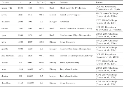
Running Time (seconds) with Increasing K

0 2 4 6 8 10 0

50

100 madelon

0 1 2 3 4 5

0 10

20 arcene

0 4 8 12 16 20 0

100

200 gina

0 4 8 12 16 20 0

50

100 secom

0 2 4 6 8 10 0

20

40 sylva

0 2 4 6 8 10 0

50

100 nova

0 3 6 9 12 15 0

100

200 gisette

0 4 8 12 16 20 0

100

200 p53

0 2 4 6 8 10 0

50

100 hiva

0 2 4 6 8 10 0

20

40 dexter

0 2 4 6 8 10 0

20

40 dorothea

0 3 6 9 12 15 0

50

100 musk

0.001 0.005 0.01 0.05 0.1

Number of Selected Variables

K Number of Selected Variables with Increasing K

(18)

the complete datasets, while for the predictive performance we used the model selection and performance estimation protocols described previously and report averages over multiple repetitions of the experiment.

Figure 1 shows how the number of runs K affects the running time and the number of selected variables. Vertical lines show the value ofKfor which the algorithm has converged (that is, after that point more runs do not select any more variables). We can see that running time increases almost linearly with an increasing number of runs K, meaning that any additional run has a roughly linear computational cost with respect to the size of the dataset. Furthermore, convergence is typically achieved in less than 10 runs, although for a few cases up to 16 runs are required. As expected, the number of selected variables increases withK, as well as with the threshold α. In the majority of cases however, most progress is made in the first few runs, and further runs increase the number of selected variables only marginally. Based on those results, we recommend considering relatively small values of K, up to K <10.

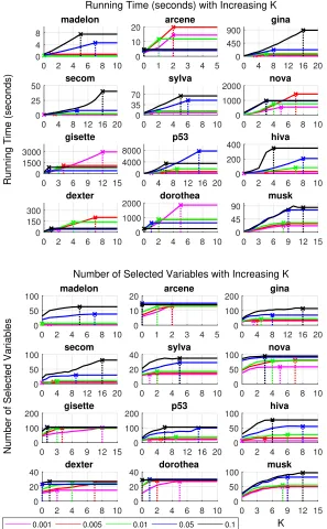
Figure 2 shows how the area under the ROC curve (AUC) varies with an increasing number of runs K, for 5 different values of the threshold parameter α of FBEDK_{. We} observe that, although AUC often tends to increase with K, this is not always the case. For instance, for the nova and dexter datasets, AUC actually decreases with K for some values of α. The maximum AUC is typically achieved with relatively small values of K, further suggesting that considering higher values forK is not necessary. Also, there are no clear relationships between AUC, the value of α and the type of predictive models used. Depending on the dataset different values ofα or predictive models may be optimal. Thus, in practice we recommend considering several combinations of α and K. Optimizing over both α andK will be considered in Section 4.4.

4.3. FBEDK vs FBS

In this section we compare FBEDK to the standard FBS algorithm in terms of predictive performance, number of selected variables and running time. The algorithms were com-pared on the same hyper-parameters (for example, FBS vs FBED0 with α = 0.01); results when also optimizing over hyper-parameters are shown in Section 4.4. Model selection and performance estimation was performed for each feature selection algorithm and each hyper-parameter value separately, following the procedure described in the experimental setup.

The main goal of this comparison is to show that FBEDK and FBS perform similarly for the same hyper-parameters, with the former being faster. A summary of the results is presented next.

(19)

0 4 8 12 16 20 59.5%

61.8%

64.0% madelon

0 2 4 6 8 10 75.5%

77.3%

79.0% arcene

0 9 18 27 36 45 91.5%

94.8%

98.0% gina

0 5 10 15 20 25 54.5%

63.5%

72.5% secom

0 3 6 9 12 15 99.5%

99.8%

100.0% sylva

0 2 4 6 8 10 90.5%

92.5%

94.5% nova

0 3 6 9 12 15 99.0%

99.3%

99.5% gisette

0 5 10 15 20 25 92.0%

93.8%

95.5% p53

0 6 12 18 24 30 61.5%

67.8%

74.0% hiva

0 2 4 6 8 10 96.0%

96.8%

97.5% dexter

0 2 4 6 8 10 81.0%

83.5%

86.0% dorothea

0 4 8 12 16 20 90.5%

95.3%

100.0% musk

0.001 0.005 0.01 0.05 0.1

Area Under the ROC Curve

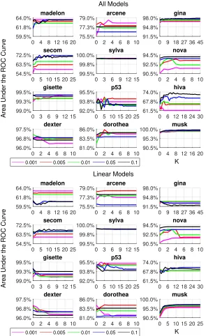
K All Models

0 4 8 12 16 20 59.5%

61.8%

64.0% madelon

0 2 4 6 8 10 75.5%

77.3%

79.0% arcene

0 9 18 27 36 45 91.5%

94.8%

98.0% gina

0 5 10 15 20 25 54.5%

63.5%

72.5% secom

0 3 6 9 12 15 99.5%

99.8%

100.0% sylva

0 2 4 6 8 10 90.5%

92.5%

94.5% nova

0 3 6 9 12 15 99.0%

99.3%

99.5% gisette

0 5 10 15 20 25 92.0%

93.8%

95.5% p53

0 6 12 18 24 30 61.5%

67.8%

74.0% hiva

0 2 4 6 8 10 96.0%

96.8%

97.5% dexter

0 2 4 6 8 10 81.0%

83.5%

86.0% dorothea

0 5 10 15 20 25 90.5%

95.3%

100.0% musk

0.001 0.005 0.01 0.05 0.1

Area Under the ROC Curve

K Linear Models

Figure 2: The figure shows how the AUC varies with an increasing number of runs K for different values of the threshold parameter α, using non-linear and linear models (top) or linear models only (bottom). There is no clear pattern for which thresholds or values ofK

to prefer, but the optimal values depend on the specific dataset, as well as on the predictive models used. However, in most cases only a few runs are required to achieve maximal AUC.

(20)

0 1 2 3 4 5 6 7 8 9 -8% -6% -4% -2% 0% 2% 4%

Area Under the ROC Curve Difference

AUC Difference of FBEDK and FBS (All Models)

mean median

0 1 2 3 4 5 6 7 8 9

-8% -6% -4% -2% 0% 2% 4%

AUC Difference of FBEDK and FBS (Linear Models)

mean median

0 1 2 3 4 5 6 7 8 9

12% 18% 25% 35% 50% 71% 100% 141% 200%

Relative Number of Selected Variables

Selected variables of FBEDK over FBS

mean median

0 1 2 3 4 5 6 7 8 9

1 2 4 8 16 32 64 128 256 512 1024 Speed-up

Speed-up of FBEDK over FBS

mean median

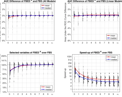
Figure 3: The x-axis of the figures on the top row shows the difference in AUC between FBEDK and FBS, with positive values indicating that FBEDK performs better than FBS. The AUC of the top left figure is computed by optimizing over all models, while for the one of the top right figure only linear models were considered. The relative number of selected variables (bottom left) shows the number of variables selected by FBEDK compared to the ones selected by FBS. The speed-up (bottom right) is computed as the one obtained by FBEDK over FBS. For all cases, the distribution over all thresholds and datasets is shown, as well as the mean and median values. The y-axis on all figures is the value of K used by FBEDK. Overall, FBEDK has a virtually identical performance with FBS, while being on average between 1 and 2 orders of magnitude faster.

difference in AUC is less than 1% while the median difference is close to 0, and for all other

K the performance is almost identical to FBS. We note that all those lower-performing cases are also the ones where FBEDK selected much fewer variables than FBS. In terms of the number of selected variables, FBEDK produces smaller solutions for K < 3, and tends to select the same number as FBS with increasing K. Finally, in terms of running time, FBEDK is significantly faster than FBS, being about 1-2 orders of magnitude faster on average in all cases.

(21)

speed and small solutions are important, FBED0 and FBED1 are good choices, as they are ∼30-100 times faster than FBS, selecting only∼70%-80% of the variables with a minimal drop in AUC. Therefore, if the number of variables is high, FBED0 and FBED1 are prefer-able due to their low computational lost. Furthermore, in low sample settings the smaller solutions of FBED0 and FBED1 are important, as selecting many variables leads to loss of power and overfitting. If on the other hand the sample size is large and the number of variables is relatively small, both FBS and FBEDK with higher values ofK are reasonable choices, with the latter being more attractive, as it is around 1 order of magnitude faster and thus can scale to higher variable sizes.

4.4. Comparison of FBEDK with other Feature Selection Methods

We performed an experiment where we also optimize over the hyper-parameter values of feature selection algorithms. The main objective of this comparison is to compare FBEDK to other feature selection algorithms in a realistic scenario, where hyper-parameter values are optimized. For this comparison we focus on the predictive performance and number of selected variables; additional results showing the running time of each algorithm can be found in Appendix D.

4.4.1. Setup

For FBEDK _{optimization is performed over the threshold}_α _{and the number of runs}_K_{. We} examine four versions of FBEDK: FBED0, FBED≤1, FBED≤3 and FBED≤∞. FBED≤K means that optimization was performed for all results up to K runs. Thus, the number of hyper-parameter configurations used were 5, 10, 20 and around 50 (for most cases) for FBED0, FBED≤1, FBED≤3 and FBED≤∞ respectively. The hyper-parameter values for FBS, MMPC and LASSO-FS are the ones described in Section 4.1.1 (a total of 100, 20 and 100 respectively). We also included results when no feature selection was performed (NO-FS). Finally, we remind the reader that we used two sets of classification algorithms and hyper-parameters, one containing only linear algorithms (elastic net regularized logistic regression) and one also containing non-linear ones in addition to the linear ones (Gaussian support vector machines and random forests). For brevity, we will refer to linear models as LM and to the combination of linear and non-linear models as NLM hereafter.

4.4.2. Results

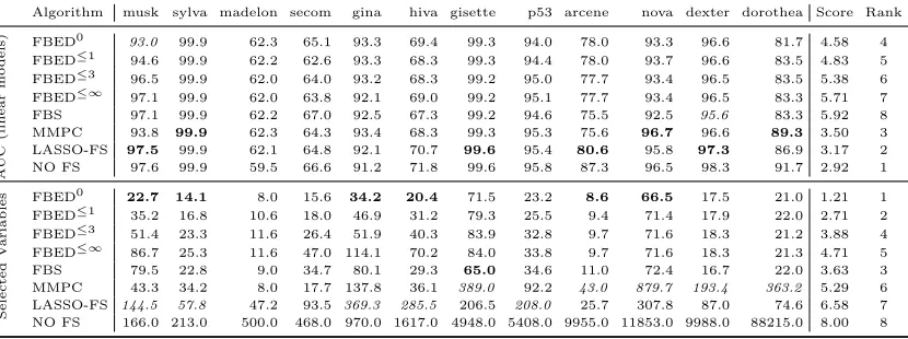
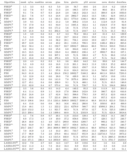
A summary of the results averaged over repetitions, measuring the AUC and number of selected variables is shown in Tables 2 and 3. For each algorithm, we computed a score which is the average rank of that algorithm over all datasets. The final rank of an algorithm is then computed based on that score. We used a bootstrap-based procedure to compute the probability of an algorithm being significantly better or worse than all competitors, and used a threshold of 95%. The procedure is described in more detail in Appendix C. In the tables, algorithms that are statistically significantly better than all others are shown in bold, whereas algorithms that are worse than the rest are shown in italic.

(22)

Table 2: Area under the ROC curve and number of selected variables for all feature selection algorithms using linear and non-linear models. The results are obtained after optimizing the hyper-parameters of the feature selection and modeling algorithms. Bold and italic entries denote that the method is significantly better or worse than all other feature selection methods (excluding NO-FS) respectively. The score is the average rank of each method over all datasets and the final rank is computed using those scores. Methods that select more variables tend to also perform better (Spearman correlation between AUC and variable rankings is -0.976).

Algorithm musk sylva madelon secom gina hiva gisette p53 arcene nova dexter dorothea Score Rank

A

UC

(all

mo

dels)

FBED0 _98.5 _99.9 _63.4 _63.7 _97.0 _67.4 _99.4 _93.3 _77.5 _93.6 _96.7 _83.8 _6.33 ₈

FBED≤1 98.7 99.9 63.3 63.0 97.3 70.9 99.4 93.5 76.9 94.0 96.8 83.5 6.17 7

FBED≤3 99.2 99.9 63.0 68.0 97.3 68.8 99.4 93.2 77.3 93.6 96.8 84.3 5.46 6

FBED≤∞ 99.5 99.9 63.6 67.6 97.6 72.3 99.4 93.5 77.3 93.6 96.8 84.9 4.71 4

FBS 99.5 99.9 64.8 69.5 97.5 69.1 99.4 94.1 77.2 92.4 95.9 84.3 5.00 5

MMPC 98.9 99.9 65.1 63.4 98.1 68.3 99.6 93.1 79.6 96.7 97.3 91.7 4.00 3

LASSO-FS 99.9 99.9 82.3 69.8 98.2 74.2 99.7 94.2 82.4 96.1 97.2 89.0 2.58 2

NO FS 99.9 99.9 82.8 71.9 98.3 74.3 99.6 94.7 90.0 96.6 98.2 94.6 1.75 1

Selected

V

ariab

les FBED

0 _22.1 _13.4 _8.4 _15.0 _32.9 _18.8 _72.9 _24.2 _8.7 _66.5 _17.4 _21.6 _1.33 ₁

FBED≤1 _35.6 _15.2 _8.2 _18.6 _47.7 _34.1 _80.2 _23.5 _9.6 _71.9 _18.0 _23.2 _2.79 ₂

FBED≤3 47.1 21.1 14.0 24.4 56.5 43.5 80.2 26.4 9.3 72.1 18.5 22.3 3.63 4

FBED≤∞ 77.6 25.5 14.9 41.1 105.8 75.1 79.4 33.7 9.3 72.3 18.7 22.4 4.79 5

FBS 76.1 21.1 19.6 28.4 78.7 33.8 65.0 32.6 11.0 71.6 16.9 22.0 3.46 3

MMPC 42.5 20.7 17.0 16.2 155.4 51.7 388.2 68.8 43.9 879.7 187.2 445.1 5.42 6 LASSO-FS 138.2 43.0 495.4 133.3 406.4 306.6 187.5 161.9 29.6 349.8 97.9 70.1 6.58 7 NO FS 166.0 213.0 500.0 468.0 970.0 1617.0 4948.0 5408.0 9955.0 11853.0 9988.0 88215.0 8.00 8

Table 3: Area under the ROC curve and number of selected variables for all feature selec-tion algorithms using linear models. The results are obtained after optimizing the hyper-parameters of the feature selection and modeling algorithms. Bold and italic entries denote that the method is significantly better or worse than all other feature selection methods (ex-cluding NO-FS) respectively. The score is the average rank of each method over all datasets and the final rank is computed using those scores. Methods that select more variables tend to also perform better (Spearman correlation between AUC and variable rankings is -0.595), but the effect is not as strong as the one of the previous results (Table 2).

Algorithm musk sylva madelon secom gina hiva gisette p53 arcene nova dexter dorothea Score Rank

A

UC

(linear

mo

dels)

FBED0 93.0 99.9 62.3 65.1 93.3 69.4 99.3 94.0 78.0 93.3 96.6 81.7 4.58 4

FBED≤1 94.6 99.9 62.2 62.6 93.3 68.3 99.3 94.4 78.0 93.7 96.6 83.5 4.83 5

FBED≤3 _96.5 _99.9 _62.0 _64.0 _93.2 _68.3 _99.2 _95.0 _77.7 _93.4 _96.5 _83.5 _5.38 ₆

FBED≤∞ 97.1 99.9 62.0 63.8 92.1 69.0 99.2 95.1 77.7 93.4 96.5 83.3 5.71 7

FBS 97.1 99.9 62.2 67.0 92.5 67.3 99.2 94.6 75.5 92.5 95.6 83.3 5.92 8

MMPC 93.8 99.9 62.3 64.3 93.4 68.3 99.3 95.3 75.6 96.7 96.6 89.3 3.50 3

LASSO-FS 97.5 99.9 62.1 64.8 92.1 70.7 99.6 95.4 80.6 95.8 97.3 86.9 3.17 2

NO FS 97.6 99.9 59.5 66.6 91.2 71.8 99.6 95.8 87.3 96.5 98.3 91.7 2.92 1

Selected

V

ariab

les FBED

0 _22.7 _14.1 _8.0 _15.6 _34.2 _20.4 _71.5 _23.2 _8.6 _66.5 _17.5 _21.0 _1.21 ₁

FBED≤1 35.2 16.8 10.6 18.0 46.9 31.2 79.3 25.5 9.4 71.4 17.9 22.0 2.71 2

FBED≤3 51.4 23.3 11.6 26.4 51.9 40.3 83.9 32.8 9.7 71.6 18.3 21.2 3.88 4

FBED≤∞ 86.7 25.3 11.6 47.0 114.1 70.2 84.0 33.8 9.7 71.6 18.3 21.3 4.71 5

FBS 79.5 22.8 9.0 34.7 80.1 29.3 65.0 34.6 11.0 72.4 16.7 22.0 3.63 3

MMPC 43.3 34.2 8.0 17.7 137.8 36.1 389.0 92.2 43.0 879.7 193.4 363.2 5.29 6

LASSO-FS 144.5 57.8 47.2 93.5 369.3 285.5 206.5 208.0 25.7 307.8 87.0 74.6 6.58 7 NO FS 166.0 213.0 500.0 468.0 970.0 1617.0 4948.0 5408.0 9955.0 11853.0 9988.0 88215.0 8.00 8

(23)

variables, LASSO-FS selects statistically significantly more in 7 and 5 cases for NLM and LM, while MMPC selects the most variables in 5 datasets for both NLM and LM. FBEDK and FBS on the other hand tend to select fewer variables. Thus, there is a clear trade-off between model interpretability (number of selected variables) and predictive performance (AUC). Specifically, there is a -0.976 and -0.595 Spearman correlation between the AUC and selected variables ranks for NLM and LM respectively. For that reason, we performed an additional experiment, comparing the AUC between FBEDK, FBS and LASSO-FS by constraining the total number of variables to select, presented in Section 4.5.

A strong outlier in the NLM case is the difference in performance of LASSO-FS com-pared to the other methods on the madelon dataset, where LASSO-FS reaches an AUC that is 17.3−19.5% higher, which is also close to the AUC of NO-FS. The main reason why all methods fail is because the madelon dataset has been constructed in a way that makes it hard for linear methods (FBEDK_{, FBS and MMPC using the logistic regression} test). Specifically, the outcome variable has been artificially constructed to be a XOR-type problem of 5 variables (Guyon et al., 2006b). Further evidence for the hardness of this problem is the fact that using LM and NO-FS achieves an AUC of only 59.5 (even lower than all feature selection methods). LASSO-FS, although also linear, is able to pick up the signal as it basically performs no feature selection, selecting 495.4 out of 500 variables on average. This happens because LASSO-FS explores up to 100 values forλ, some of which correspond to very dense solutions. In contrast, due to the experimental setup, none of the remaining methods selects that many variables in this case.

An interesting observation is the fact that FBED0 and FBED≤1, the forward selection methods selecting the fewest variables, are ranked higher in terms of AUC than FBED≤3, FBED≤∞and FBS when using LM. Thus, they are better suited to pick out linear trends in the data, producing solutions that are smaller and more predictive compared to algorithms of the same type. Using NLM gives an even bigger advantage to methods selecting more variables, as this increases the chance to also capture some non-linear signals in the data.

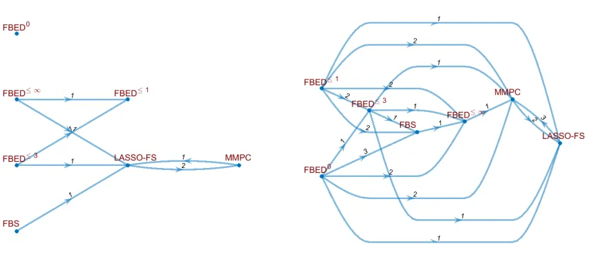
Finally, we performed a statistical test between all pairs of methods to identify cases where a method outperforms others, both in terms of AUC and number of selected variables. Again, we used a bootstrap-based test, computing the joint probability that methodAhas a higher AUC and selecting fewer variables than method B, using the same procedure as described in Appendix C. A method is considered to dominate another, if that probability is higher than 95%. The results are summarized in Figure 4. Each node corresponds to a feature selection method, and a directed edge from method A to B with weight w

(24)

(a) Dominating Relationships (All Models) (b) Dominating Relationships (Linear Models)

Figure 4: The figures show how often a feature selection method dominates another (that is, has a higher AUC while selecting fewer variables), using non-linear models (left) and linear models (right). An edge from method AtoB with weight windicates thatA dominatesB

in w datasets. Except for FBED≤∞ for linear models, which gets dominated by FBS in 1 dataset, methods in the FBEDKfamily are never dominated by FBS, MMPC or LASSO-FS, while typically dominating them in 1-3 datasets.

Overall, there is no clear winner, and the choice depends solely on the goal. If the goal is predictive performance, LASSO-FS or MMPC are clearly preferable. If on the other hand one is interested in interpretability, then methods from the FBEDK _{family with small} values ofK are preferable. Regarding FBS, there is no scenario where it is preferable over one of the other algorithms. We must note that those results are somewhat artificial, as the performance of FBEDK and FBS highly depends on the hyper-parameter values chosen for the experiment, while LASSO-FS is not as sensitive to those choices. Furthermore, the fact that hyper-parameters are optimized based on performance naturally tends to favor methods that select more variables, putting LASSO-FS at a disadvantage in terms of interpretability.

4.5. Fixing the Number of Selected Variables

As confirmed by the previous experiment, there are two main trade-offs for feature selection algorithms: (a) the number of selected variables, with fewer variables leading to more inter-pretable results, and (b) the predictive ability of the selected variables, with more variables typically leading to better results. In general, algorithms that select more variables also tend to perform better in terms of predictive performance. Because of that,we performed a comparison where algorithms are forced the select the same number of variables. That way, the predictive performance of algorithms can be compared on equal footing.

(25)

0 1 2 3 4 5 6 7 8 9 -15%

-10% -5% 0% 5% 10%

AUC Difference of FBEDK and LASSO-FS (All Models)

mean

median

0 1 2 3 4 5 6 7 8 9

-15% -10% -5% 0% 5% 10%

AUC Difference of FBEDK and LASSO-FS (Linear Models)

mean median

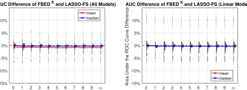
Figure 5: LASSO-FS with limit on selected variables: The x-axis shows the distri-bution of the difference in AUC of FBEDK and LASSO-FS, with positive values indicating that FBEDK performs better. The y-axis corresponds to value of K used by FBEDK. The mean and median values are shown in red and blue respectively. The average difference using non-linear models is 0.78%, and 0.23% when using only linear models. The difference can be explained by the arcene dataset, where LASSO-FS outperforms FBEDK even when selecting the same number of variables. A more detailed explanation is given in the main text.

Section 4.3 that FBS and FBEDK exhibit similar predictive performance with a similar number of selected features, with FBEDK being orders of magnitude faster. MMPC was not included, because neither MMPC nor FBEDK _{allow to set the number of features to} select.

In order to perform the comparison, we executed FBEDK for multiple hyper-parameter values (the ones given in the experimental setup) and then executed LASSO-FS with the constraint to select the same number of variables as FBEDK did. As it was not always possible to select the exact same number of variables, we identified the solution of LASSO-FS with at least as many variables as FBEDK. Except for a few cases where LASSO-FS selected 1 more variable than FBEDK, both methods selected the same number of variables. As a final comment, we note that the above experiment does not favor FBEDK over LASSO-FS, as no optimization over its hyper-parameter values is performed. The reason we did not use a fixed number of variables M to select is because there is no easy way to select exactlyM variables using FBEDK.

(26)

0.23%. In terms of median difference in AUC, a metric which is more stable with the re-spect to the datasets and hyper-parameter values used, both algorithms perform almost identically. Those results also agree with previous comparisons between forward selection and LASSO-FS (Hastie et al., 2017).

We investigated the difference in performance and found that it can be attributed to the arcene dataset. By removing this dataset, LASSO-FS outperforms FBEDK by 0.32% on average using non-linear models, while for linear models FBEDK performs better by 0.22%. Note that, arcene is the dataset which contains the fewest number of samples, while also containing a large number of variables. It contains 200 samples and 10000 variables, and only 120/160 are used for training and validation respectively. Theoretical results by Ng (2004) show that LASSO performs well in settings with low sample size and many irrelevant variables, as is the case for the arcene dataset. One possible explanation for the lower performance of FBEDKon arcene is that forward selection based procedures use more effective degrees of freedom (Hastie et al., 2017, Figure 1), thus requiring more sample size to have sufficient statistical power to pick up weak signals. It would be interesting to study this effect in more depth, but it is out of the scope of the current paper. In summary,

LASSO-FS and FBEDK perform similarly when the number of variables to select is the same.

4.6. Simulation Study on the Multiple Testing Problem

The idea of early dropping of variables used by FBEDK _{does not only reduce the running} time, but also reduces the problem of multiple testing, in some sense. Specifically, it reduces the number of variables falsely selected due to type I errors. In general, the number of false selections is related to the total number of variables considered in all forward iterations. Thus, the effect highly depends on the value of K used by FBEDK, with higher values of K leading to more false selections. We show this for FBED0 by considering a simple scenario, where none of the candidate variables are predictive for the outcome. Then, in the worst case, FBED0 will select aboutα·pof the variables on average (where α is the significance level), since all other variables will be dropped in the first iteration. This stems from the fact that, under the null hypothesis of conditional independence, the p-values are uniformly distributed. In practice, the number of selected variables will be even lower, as FBED0 will keep dropping variables after each variable inclusion. On the other hand, FBS may select a much larger number of variables, since each variable is given the chance to be included in the output at each iteration and will often do so, simply by chance.

We performed a small simulation to investigate the behavior of FBED0_{, FBED}1_{, FBED}∞

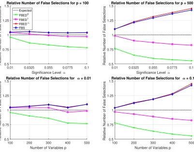
and how they compare to FBS. We generated 500 normally distributed datasets with 1000 samples each, a uniformly distributed random binary outcome, and considered different variable sizes p ∈ {100,200,300,400,500} and 5 significance levels α uniformly spaced in [0.01,0.1]. All variables are generated randomly, and there is no dependency between any of them. Thus, a false positive rate of about α is expected, if no adjustment is done to control the false discovery rate. For each setting, we computed the ratio of false positives with respect to the expected number of false positives.

(27)

0.01 0.0325 0.055 0.0775 0.1

Significance Level

0.5 0.75 1 1.25 1.5

Relative Number of False Selections

Relative Number of False Selections for p = 100

Expected FBED0 FBED1 FBED FBS

100 200 300 400 500

Number of Variables p 0.5

0.75 1 1.25 1.5

Relative Number of False Selections for = 0.01

0.01 0.0325 0.055 0.0775 0.1

Significance Level

0.5 0.75 1 1.25 1.5

Relative Number of False Selections for p = 500

100 200 300 400 500

Number of Variables p 0.5

0.75 1 1.25 1.5

Relative Number of False Selections for = 0.1

Figure 6: The figures show the relative number of false selections by each algorithm on randomly generated data. The expected number of false selections is α·p, where α is the significance level and p the number of variables. The numbers are computed as the ratio between the average number of selected variables to the expected false positives. FBED0 and FBED1typically select fewer variables than expected, and their behavior improves with increasingαandp. FBED∞and FBS on the other hand select more false positive variables, getting worse with larger values of α or on datasets with more variables.

of variables. In all cases, FBED0 and FBED1 select fewer false positives than expected, and their behavior improves both with increasing αand number of variables. FBED∞ and FBS perform almost identically, and tend to select more variables. We also observe that the number of false positives increases both withα and with the number of variables. Thus,in case one is interested to limit the number of false selection, we recommend running FBEDK with a small value of K.

5. Conclusion

(28)

theoretical guarantees of forward-backward selection. We prove that FBED1 and FBED∞ identify the optimal solution (Markov blanket) if the distribution of the data can be faith-fully represented by a Bayesian network or maximal ancestral graph respectively, similar to the standard forward-backward selection (FBS).

A useful property of FBEDK is that it is a general algorithm that can be adapted to han-dle different variable types (for example, continuous, categorical, ordinal), cross-sectional and time-course data, linear and non-linear dependencies, as well as different analysis tasks (for example, regression, classification, survival analysis) by using an appropriate condi-tional independence test. In contrast, algorithms like LASSO (Tibshirani, 1996), although being computationally fast and performing well in terms of predictive performance for com-mon problems like regression and classification, are not as general (Meier et al., 2008; Schelldorfer et al., 2011; Ivanoff et al., 2016) and are computationally demanding for some problems (Fan et al., 2010; Groll and Tutz, 2014; Tsagris et al., 2018).

In experiments we demonstrate that FBEDK behaves similarly to FBS in terms of pre-dictive performance and number of selected variables, while being 1-2 orders of magnitude faster. Compared to other feature selection algorithms like LASSO (Tibshirani, 1996) and MMPC (Tsamardinos et al., 2003a), FBEDKhas competitive predictive performance, while selecting the fewest variables, which is especially important if feature selection is performed for knowledge discovery. An interesting result is that FBEDK and LASSO perform about equally well, when limited to select the same number of variables. This, combined with the fact that FBEDK is more general, makes it an attractive alternative to LASSO, especially for problems where no efficient solution to the LASSO problem exists.

Acknowledgments

We would like to thank Vincenzo Lagani and Michalis Tsagris for their helpful comments. This work was funded by the European Research Council under the European Union’s Seventh Framework Programme (FP/2007-2013) / ERC Grant Agreement n. 617393.

Appendix A. Bayesian Networks and Maximal Ancestral Graphs

We will briefly introduce Bayesian networks and maximal ancestral graphs, which we will use to show theoretical properties of FBEDK.

A directed acyclic graph (DAG) is a graph that only contains directed edges (→) and has no directed cycles. A directed mixed graph is a graph that, in addition to directed edges also contains bi-directed edges (↔). The graphs contain no self-loops, and vertices can be connected only by a single edge. Two vertices are calledadjacent if they are connected by an edge. An edge betweenX andY is calledintoY ifX→Y orX↔Y. A path in a graph is a sequence of unique verticeshV1, . . . , Vki such that each consecutive pair of vertices is adjacent. The first and last vertices in a path are called endpoints. A path is called directed if ∀1 ≤ i ≤ k, Vi → Vi+1. If X → Y is in a graph, then X is a

parent of Y and Y a child of X. A vertex W is aspouse of X, if both share a common child. A vertex X is an ancestor of Y, andY is a descendantof X, if X =Y or there is a directed path from X toY. A triplet hX, Y, Zi is called a collider ifY is adjacent to