Assessing discriminative ability of risk models in clustered data

R E S E A R C H A R T I C L E

Open Access

Assessing discriminative ability of risk models in

clustered data

David van Klaveren

, Ewout W Steyerberg

, Pablo Perel

and Yvonne Vergouwe

Abstract

Background:The discriminative ability of a risk model is often measured by Harrell’s concordance-index (c-index). The c-index estimates for two randomly chosen subjects the probability that the model predicts a higher risk for the subject with poorer outcome (concordance probability). When data are clustered, as in multicenter data, two types of concordance are distinguished: concordance in subjects from the same cluster (within-cluster concordance probability) and concordance in subjects from different clusters (between-cluster concordance probability). We argue that the within-cluster concordance probability is most relevant when a risk model supports decisions within clusters (e.g. who should be treated in a particular center). We aimed to explore different approaches to estimate the within-cluster concordance probability in clustered data.

Methods:We used data of the CRASH trial (2,081 patients clustered in 35 centers) to develop a risk model for mortality after traumatic brain injury. To assess the discriminative ability of the risk model within centers we first calculated cluster-specific c-indexes. We then pooled the cluster-specific c-indexes into a summary estimate with different meta-analytical techniques. We considered fixed effect meta-analysis with different weights (equal; inverse variance; number of subjects, events or pairs) and random effects meta-analysis. We reflected on pooling the estimates on the log-odds scale rather than the probability scale.

Results:The cluster-specific c-index varied substantially across centers (IQR= 0.70-0.81;I2= 0.76 with 95% confidence interval 0.66 to 0.82). Summary estimates resulting from fixed effect meta-analysis ranged from 0.75 (equal weights) to 0.84 (inverse variance weights). With random effects meta-analysis–accounting for the observed heterogeneity in c-indexes across clusters–we estimated a mean of 0.77, a between-cluster variance of 0.0072 and a 95% prediction interval of 0.60 to 0.95. The normality assumptions for derivation of a prediction interval were better met on the probability than on the log-odds scale.

Conclusion:When assessing the discriminative ability of risk models used to support decisions at cluster level we recommend meta-analysis of cluster-specific c-indexes. Particularly, random effects meta-analysis should be considered.

Keywords:Clustered data, Concordance, Discrimination, Meta-analysis, Prediction, Risk model

Background

Assessing the performance of a risk model is of great practical importance. An essential aspect of model per-formance is separating subjects with good outcome from subjects with poor outcome (discrimination) [1]. The concordance probability is a commonly used measure of discrimination reflecting the association between model predictions and true outcomes [2,3]. For binary outcome

data it is the probability that a randomly chosen subject from the event group has a higher predicted probability of having an event than a randomly chosen subject from the non-event group. For time-to-event outcome data it is the probability that, for a randomly chosen pair of subjects, the subject who experiences the event of interest earlier in time has a lower predicted value of the time to the occurrence of the event. For both kinds of outcome data the concordance probability is often estimated with Harrell’s concordance (c)-index [2].

* Correspondence:[email protected]

1

Department of Public Health, Erasmus MC, Dr. Molewaterplein 50, Rotterdam 3015 GE, The Netherlands

Full list of author information is available at the end of the article

In risk modelling, clustered data are frequently used. A typical example is multicenter patient data, i.e. data of patients who are treated in different centers with similar inclusion criteria across the centers. Patients treated in the same center are nevertheless more alike than patients from different centers. A comparable type of clustering may occur in patients treated in different countries or in patients treated by different caregivers in the same center. Similarly, in public health research the study population is often clustered in geographical regions like countries, municipalities or neighbourhoods. It has been suggested that clustering should be taken into account in the devel-opment of risk models to obtain unbiased estimates of predictor effects [4]. This can be done by using a multi-level logistic regression model for binary outcomes or a frailty model for time-to-event outcomes [5,6].

It would be natural to take clustering also into account when measuring the performance of a risk model. For multilevel models, it has been proposed to consider the concordance probability of subjects within the same clus-ter (within-clusclus-ter concordance probability) separately from the concordance probability of subjects in different clusters (between-cluster concordance probability) [7,8]. We propose using the within-cluster concordance prob-ability when risk models are used to support decisions within clusters, e.g. in clinical practice where decisions on interventions are commonly taken within centers. A valu-able risk model should then be valu-able to separate subjects within the same cluster into those with good outcome and poor outcome. We consider the within-cluster con-cordance probability more relevant in this context than the between-cluster or overall concordance probability.

Here, we aimed to estimate the within-cluster concord-ance probability from clustered data. We explored different meta-analytic methods for pooling cluster-specific concord-ance probability estimates with an illustration in predicting mortality among patients suffering from traumatic brain injury.

Methods

Mortality in traumatic brain injury patients

We present a case study of predicting mortality after Traumatic Brain Injury (TBI). Risk models using baseline characteristics provide adequate discrimination between patients with good and poor 6-month outcomes after TBI [9,10]. We used patients enrolled in the Medical Research Council Corticosteroid Randomisation after Significant Head Injury [11] trial (registration ISRCTN74459797, http://www.controlled-trials.com/), who were recruited between 1999 and 2004. This was a large international double-blind, randomized placebo-controlled trial of the effect of early administration of a 48-h infusion of methylprednisolone on outcome after head injury. The trial included 10,008 adults clustered in 239 centers

with Glasgow Coma Scale (GCS) [12] Total Score≤14, who were enrolled within 8 hours after injury. By design the patient inclusion criteria were equal in all 239 centers.

We considered patients with moderate or severe brain injury (GCS Total Score≤12) and observed 6-month Glasgow Outcome Scale (GOS) [13]. Patients who were treated in one of 35 European centers with more than 5 patients experiencing the event (n= 2,081), were used to assess the discriminative ability of a prediction model developed with data from 35 centers. Patients who were treated in one of 21 Asian centers with more than 5 patients experiencing the event (n= 1,421) were used to assess the discriminative ability at external validation.

We used a Cox proportional hazards model with age, GCS Motor Score and pupil reactivity as covariates similar to previously developed risk models [9,10]. We modelled center with a Gamma frailty (random effect) to account for heterogeneity in mortality among centers. We esti-mated parameters on the European selection of patients with the R package survival [14,15]. As center effect estimates are unavailable when using a risk model in new centers, we calculated individual risk predictions applying the Gamma frailty mean of 1 for each patient.

Cluster-specific concordance probabilities

We estimated the concordance probability within each cluster by Harrell’s c-index [2], i.e. the proportion of all usable pairs of subjects in which the predictions are con-cordant with the outcomes. A pair of subjects is usable if we can determine the ordering of their outcomes. For binary outcomes, pairs of subjects are usable if one of the subjects had an event and the other did not. For time-to-event outcomes, pairs of subjects are usable if their failure times are not equal and at least the smallest failure time is uncensored. For a usable subject pair the predictions are concordant with the outcomes if the or-dering of the predictions is equal to the oror-dering of the outcomes. Values of the c-index close to 0.5 indicate that the model does not perform much better than a coin-flip in predicting which subject of a randomly chosen pair will have a better outcome. Values of the c-index near 1 indicate that the model is almost perfectly able to predict which subject of a randomly chosen pair will have a favourable outcome. We estimated the variances of the cluster-specific c-indexes with a method proposed by Quade [16]. Formulas are provided in Appendix 1.

Pooling cluster-specific concordance probability estimates

The within-cluster concordance probability Cw can be

weights [7,8]. Here, we define eight different ways for pooling of cluster-specific estimates–both on the prob-ability scale and on the log-odds scale–based on fixed effect meta-analysis and random effects meta-analysis.

We consider a dataset with subjects inKclusters. Letmk

be the number of subjects andekbe the number of events in

clusterk. We denote the number of usable subject pairs – pairs of subjects for whom we can determine the ordering of their outcomes–in clusterkbynk. The cluster-specific

concordance probability estimate for clusterkis denoted byC^kwith sampling variance estimateσ^2k.

Fixed effect meta-analysis

Fixed effect meta-analysis assumes that one common within-cluster concordance probability CW exists that

applies to all clusters. The observed cluster-specific esti-mates vary only because of chance created from sampling subjects. Fixed effect meta-analysis with cluster weightswk

results in:

^

CW ¼

X

kwkC^k

X

kwk

withσ^2_C^

W ¼

X

kw 2 kσ^2k

X

kwk

2 ð1Þ

The simplest approach would be to apply equal weights, wk = 1/K for each cluster (method 1). This estimator is

quite naive when the cluster size varies, because small clusters are given the same weight as large clusters and information about the precision of the cluster-specific estimates is ignored. Heuristic choices of weights taking the cluster size into account are the number of subjects, wk =mk (method 2), or the number of events, wk =ek

(method 3). Analogous to the definition of the c-index a fourth option is the number of usable subject pairs as weights, wk = nk (method 4). The pooled estimate is

then equal to the proportion of all usable within-cluster subject pairs in which the predictions and outcomes are concordant. Another choice of meta-analysis weights are the inverse variances, wk ¼1=σ^2k (method 5). These weights express the precision of the cluster-specific esti-mates and are commonly used in meta-analysis of study-specific treatment effects.

Random effects meta-analysis

In our context a random effects meta-analysis considers that the cluster-specific estimates vary not only because of sampling variability but also because of differences in true concordance probabilities. This is appropriate for high values of I2 [17]. I2 measures the proportion of variability in cluster-specific estimates that is due to between-cluster heterogeneity rather than chance. Ran-dom effects meta-analysis assumes that cluster-specific concordance probabilitiesCkare distributed about meanμ

with between-cluster variance τ2, with the observed C^k

normally distributed aboutCkwith sampling variance σ2k. The mean within-cluster concordance probability estimate ^

μ is the average of the cluster-specific estimates with the inverse variances as weights (method 6):

^

μ¼

X

kwkC^k

X

kwk ;σ^2

^ μ ¼

X

kw 2 k σ^

2 kþ^τ

2

X

kwk

2

¼X1

kwk

with wk¼1= σ^2kþτ^2

ð2Þ

For estimation of the between-cluster varianceτ2we used the DerSimonian and Laird [18] method. Alternative estima-tors forτ2can be found in DerSimonian and Kacker [19].

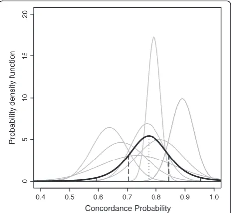
With the additional assumption of normally distributed Ck we can derive a prediction interval for the

within-cluster concordance probabilityCW in a new or

unspeci-fied cluster [20]. Ifτ2were known, thenμ^_eN μ;σ^2^μ

and CW~N(μ,τ2) imply (assuming independence ofCWandμ^

givenμ) that CW−μ^eN 0;τ2þσ^2μ^

. Hence the

within-cluster concordance probability CW in a new cluster is

normally distributed, with mean μ^ and variance τ2_þσ^2 ^

μ (Figure 1). Since τ2 is estimated, we assume CffiffiffiffiffiffiffiffiffiffiW−μ^

^

τ2_þ^σ2

^ μ

p to

take a more conservative t-distribution withK- 2 degrees of freedom instead of the standard normal distribution

0.4 0.5 0.6 0.7 0.8 0.9 1.0

10

5

01

5

2

0

Concordance Probability

Probability density function

[20]. Thus, a 95% prediction interval of the within-cluster concordance probabilityCW in an unspecified cluster can

be approximated by:^μt0K:975−2

ffiffiffiffiffiffiffiffiffiffiffiffiffiffiffiffi ^ τ2_þσ^2

^

μ q

witht0K:−9752

denot-ing the 97.5% percentile of the t-distribution withK- 2 de-grees of freedom.

Meta-analysis scale

When calculating a prediction interval of the within-cluster concordance probabilityCW, Riley et al [21]

ad-vised to perform a random effects meta-analysis on a scale that helps meet the normality assumption for the random effects. When the normality assumption of the random effects model holds, the Ck are normally

distrib-uted with meanμand varianceτ2_þσ2

k. As a consequence, the standardized residuals zk defined below should

ap-proximately have a standard normal distribution:

zk¼ C^k−^μ

= ffiffiffiffiffiffiffiffiffiffiffiffiffiffiffiffi^τ2_þσ^2 k

q

ð3Þ

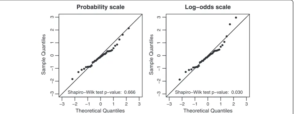
To consider if the normality assumption is valid we used a normal probability plot of zk and applied the

Shapiro-Wilk test tozk[22]. In a normal probability plot

zk is plotted against a theoretical normal distribution in

such a way that the points should form an approximate straight line. Departures from this straight line indicate departures from normality. The Shapiro-Wilk test returns the probability of obtaining the test-statistic as least as ex-treme as the observed one, under the null-hypothesis that zkare normally distributed (p-value). When the p-value is

above significance levelα, say 5%, the null hypothesis that zkis normally distributed is not rejected.

Since the concordance probability is restricted to [0, 1] the normality assumption of random effects meta-analysis may be violated. We considered inverse variance weighted meta-analysis on the log-odds scale as an alternative

approach (methods 7 and 8 for fixed effect and random ef-fects meta-analysis respectively). The resulting estimators for the within-cluster concordance probability are defined in Appendix 2. The normality assumption on log-odds scale was again assessed by the normal probability plot and the Shapiro-Wilk test.

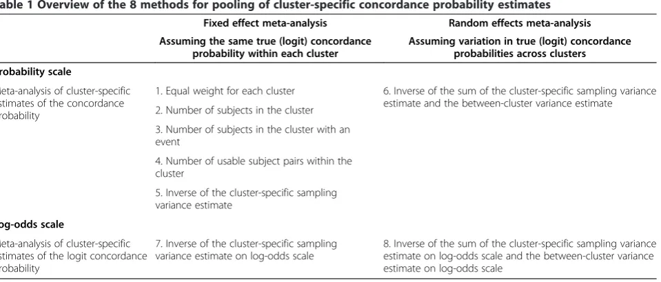
Table 1 contains a summary of the eight pooling meth-odologies described above. For all the meta-analyses we used the R package rmeta [14,23].

Results

The European patients were slightly older in comparison with the Asian patients (median age 36 vs. 31 years) and were more likely to have the worst GCS Motor Score of 1, i.e. no motor response (21% versus 4%) compared to the Asian patients (Table 2). However, 6 month mortality was lower in the European patients (27%) than in the Asian patients (35%).

We found that 6-month mortality was clearly associated with higher age, worse GCS Motor Score and less pupil reactivity (Table 3). Heterogeneity in mortality among European centers was substantial as indicated by the hazard ratio of 1.7 for the 75 percentile versus the 25 percentile of the random center effect, based on the quar-tiles of the Gamma frailty distribution with mean 1 and variance estimate 0.146.

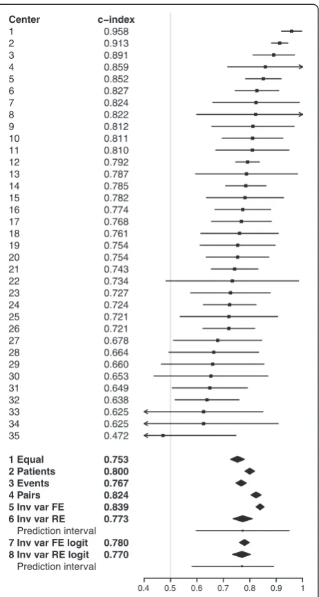
Among European centers (overall index 0.80) the c-indexes varied substantially with an interquartile range of 0.70 to 0.81 (Figure 2). Pooled concordance probability estimates resulting from fixed effect meta-analysis ranged from 0.75 (equal weights) to 0.84 (inverse variance weights). Random effects meta-analysis (method 6) led to a mean concordance probability estimate μ^¼0:77 , a between-cluster variance estimate τ^2_{¼0:0072 and a wide 95%}

prediction interval (0.60 to 0.95) reflecting the strong

Table 1 Overview of the 8 methods for pooling of cluster-specific concordance probability estimates

Fixed effect meta-analysis Random effects meta-analysis

Assuming the same true (logit) concordance probability within each cluster

Assuming variation in true (logit) concordance probabilities across clusters

Probability scale

Meta-analysis of cluster-specific estimates of the concordance probability

1. Equal weight for each cluster 6. Inverse of the sum of the cluster-specific sampling variance estimate and the between-cluster variance estimate 2. Number of subjects in the cluster

3. Number of subjects in the cluster with an event

4. Number of usable subject pairs within the cluster

5. Inverse of the cluster-specific sampling variance estimate

Log-odds scale

Meta-analysis of cluster-specific estimates of the logit concordance probability

7. Inverse of the cluster-specific sampling variance estimate on log-odds scale

heterogeneity in the cluster-specific concordance prob-abilities (I2= 0.76 with 95% confidence interval 0.66 to 0.82). Random effects meta-analysis on log-odds scale (method 8) led to similar results, but with a somewhat smaller asymmetric prediction interval (0.58 to 0.89).

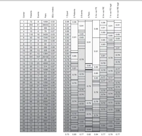
Large differences in pooling weights, together with heterogeneity in the cluster-specific concordance prob-abilities, led to very different pooled estimates. We ana-lysed the pooling weights to explain the differences in pooled estimates (Figure 3). The patient-weighted estimate was dominated by center 2 with 494 of the 2,081 patients. The event-weighted estimate was dominated by center 12 with 107 out of 553 events. The patient-pair-weighted esti-mate was heavily determined by both center 2 and center 12 as the number of usable patient pairs is related to the number of patients times the number of events. The fixed effect inverse-variance weighted estimate was also strongly influenced by centers with high number of patients or

events, because the standard errors of the cluster-specific estimates depend heavily on the number of patients and events. Furthermore, the fixed effect inverse-variance weighted estimate was upwardly influenced by center 1 as a result of the small standard error relative to the small number of patients and events. The random ef-fects inverse-variance weighted estimate was much less dominated by particular centers and close to the equally weighted estimate because of the large amount of hetero-geneity. The standard error on the log-odds scale in-creased with increasing c-index according to Equation 10 in Appendix 2 and therefore put less weight on the centers with a high concordance probability estimate resulting in lower pooled estimates. The large standard errors for centers with high c-index also decreased the heterogeneity (I2 = 0.61 with 95% confidence interval 0.44 to 0.73) on the log-odds scale resulting in more similar weights for fixed effect and random effects meta-analysis.

To check the validity of the normality assumption in the random effects meta-analyses, we calculated standardized residuals (Equation 3), both on the probability and the log-odds scale. The standardized residuals better fitted to the standard normal distribution on the probability scale than on the log-odds scale (Figure 4, p-values for rejection of the normality null hypothesis of 0.666 on probability scale and of 0.030 on log-odds scale).

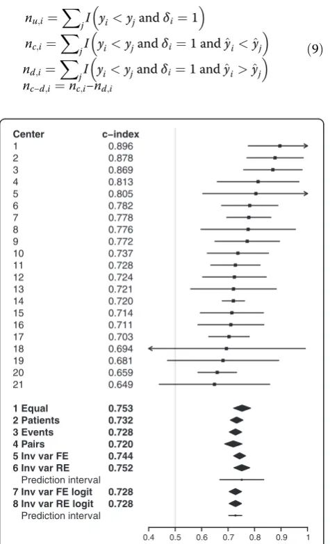
To illustrate the comparison in an external validation setting, we repeated the analysis of the within-cluster concordance probability in Asian centers with the same risk model (Figure 5). Among Asian clusters (overall c-index 0.74) the c-indexes varied less (IQR0.71-0.78), which was reflected in a lower proportion of variation among clusters that is due to heterogeneity rather than chance (I2= 0.32 with 95% confidence interval 0 to 0.60). As a result, different pooling methodologies led to more Table 2 Patient characteristics in selected European and Asian centers

Characteristic Measure or Category Europe Asia

Age (years) Median (25–75 percentile) 36 (24–53) 31 (22–43)

GCS Motor score No response (1) 445 (21%) 55 (4%)

Extension (2) 134 (6%) 96 (7%)

Abnormal flexion (3) 176 (8%) 124 (9%)

Normal flexion (4) 321 (15%) 261 (18%)

Localizes/obeys (5/6) 1,005 (48%) 885 (62%)

Pupil reactivity No pupil reacted 291 (14%) 129 (9%)

One pupil reacted 123 (6%) 117 (8%)

Both pupils reacted 1,667 (80%) 1,175 (83%)

Six-month mortality Dead 553 (27%) 495 (35%)

Patients Total 2,081 1,421

Centers Total 35 21

Patients per center Median (25–75 percentile) 33 (21–64) 34 (20–66)

Table 3 Associations between predictors and 6-month mortality in European centers

Characteristic Level HR (95 % CI)

Age (years) 47 versus 23* 2.1 (1.9-2.4)

GCS Motor score No response (1) 3.1 (2.4-4.0)

Extension (2) 2.8 (2.0-3.8)

Abnormal flexion (3) 2.4 (1.7-3.2)

Normal flexion (4) 1.5 (1.1-2.0)

Localizes/obeys (5/6) 1.0 (ref)

Pupil reactivity No pupil reacted 2.8 (2.3-3.5)

One pupil reacted 1.7 (1.2-2.3)

Both pupils reacted 1.0 (ref)

Center random effect 75 versus 25 percentile 1.7

similar pooled estimates, because differences in cluster weights have less impact when cluster-specific estimates are more alike. Based on random effects meta-analysis, es-timates of the mean within-cluster concordance probabil-ity and the between-cluster variance were μ^¼0:75 and

^

τ2_{¼0:0013 respectively. The resulting prediction interval}

(0.67 to 0.83) was much smaller than for the European clusters. The heterogeneity disappeared on the log-odds scale (I2= 0) leading to equal estimates by fixed effect and random effects meta-analysis.

Discussion

We studied how to assess the discriminative ability of risk models in clustered data. The within-cluster concordance probability is an important measure for risk models when these models are used to support decisions on interven-tions within the clusters. The within-cluster concordance probability can be estimated by pooling cluster-specific concordance probability estimates (e.g. c-indexes) with a meta-analysis, similar to pooling of study-specific treat-ment effect estimates. We considered different pooling strategies (Table 1) and recommend random effects meta-analysis in case of substantial variability–beyond chance–of the concordance probability across clusters [20,21]. To decide if the meta-analysis should be under-taken on the probability scale or the log-odds scale we suggest considering the normality assumptions on both scales by normal probability plots and Shapiro-Wilk tests of the standardized residuals.

The illustration of predicting 6-month mortality after TBI prompted the use of random effects meta-analysis because of the strong difference – beyond chance – in concordance probability among centers. This was clearly visualized by the forest plot in Figure 2. Random effects meta-analysis results can be summarized by the mean concordance probability and a 95% prediction interval for possible values of the concordance probability. By definition, these results give insight into the variation of the discriminative ability among centers as opposed to fixed effect meta-analysis results [20,21]. By comparing normal probability plots and Shapiro-Wilk test results based on the standardized residuals we concluded the random effects meta-analysis results on probability scale to be the most appropriate (Figure 4). Although the methodology is illustrated with time-to-event outcomes of traumatic brain injury patients, it is also applicable to binary outcomes.

Even if a risk model contains regression coefficients that are optimal for the data in each cluster, differences in case mix may lead to different concordance probabil-ities across clusters [24]. Furthermore, predictor effects may vary because of cluster-specific circumstances, also leading to different cluster-specific concordance prob-abilities. Given the variability beyond chance in our case study, we consider a random effects meta-analysis of the cluster-specific c-indexes as most appropriate.

The assumption of random effects meta-analysis is that underlying concordance probabilities among clusters are

Center

1 2 3 4 5 6 7 8 9 10 11 12 13 14 15 16 17 18 19 20 21 22 23 24 25 26 27 28 29 30 31 32 33 34 35

1 Equal 2 Patients 3 Events 4 Pairs 5 Inv var FE 6 Inv var RE

Prediction interval

7 Inv var FE logit 8 Inv var RE logit

Prediction interval

c−index

0.958 0.913 0.891 0.859 0.852 0.827 0.824 0.822 0.812 0.811 0.810 0.792 0.787 0.785 0.782 0.774 0.768 0.761 0.754 0.754 0.743 0.734 0.727 0.724 0.721 0.721 0.678 0.664 0.660 0.653 0.649 0.638 0.625 0.625 0.472

0.753 0.800 0.767 0.824 0.839 0.773

0.780 0.770

0.4 0.5 0.6 0.7 0.8 0.9 1

exchangeable, i.e. cluster-specific concordance probabil-ities are expected to be non-identical, yet identically distributed [20]. If part of the variation can be explained by cluster characteristics, a meta-regression–assuming partial exchangeability–of the concordance probability estimates with cluster characteristics as covariates is preferable.

We chose to analyse the concordance probability as it is the most commonly used measure of discriminative ability of a risk model. However, the same logic of pool-ing cluster-specific performance measure estimates can be applied to any other performance measure, like the discrimination slope, the explained variation (R2) or the Brier score [25].

0.75 0.80 0.77 0.82 0.84 0.77 0.78 0.77

Center Patients Events Pa

irs

SE(c−index) 1 Equal 2 Patients 3 Events 4 P

a

irs

5 Inv var FE 6 Inv var RE 7 In var FE logit 8 Inv var RE logit

35 34 33 32 31 30 29 28 27 26 25 24 23 22 21 20 19 18 17 16 15 14 13 12 11 10 9 8 7 6 5 4 3 2 1 12 16 11 103 31 12 31 19 71 66 21 57 34 25 122 50 23 33 41 45 30 110 11 181 61 28 26 11 21 53 116 10 34 494 72 7 6 7 21 19 6 8 8 14 25 6 25 12 6 31 16 11 7 13 14 11 25 7 107 13 13 6 6 8 18 16 6 6 41 8 106 144 96 3834 766 98 420 226 1760 2594 208 2118 630 218 6294 1292 358 402 872 1038 514 4808 80 26132 1384 528 266 90 244 1540 3428 78 366 38550 1058 0.14 0.11 0.14 0.06 0.07 0.11 0.10 0.09 0.09 0.05 0.09 0.05 0.08 0.13 0.05 0.06 0.07 0.07 0.06 0.05 0.07 0.04 0.10 0.02 0.07 0.06 0.08 0.11 0.08 0.04 0.03 0.07 0.04 0.02 0.02 0.47 0.62 0.62 0.64 0.65 0.65 0.66 0.66 0.68 0.72 0.72 0.72 0.73 0.73 0.74 0.75 0.75 0.76 0.77 0.77 0.78 0.79 0.79 0.79 0.81 0.81 0.81 0.82 0.82 0.83 0.85 0.86 0.89 0.91 0.96 0.64 0.68 0.72 0.74 0.79 0.79 0.81 0.85 0.91 0.96 0.64 0.65 0.72 0.72 0.74 0.75 0.79 0.79 0.83 0.85 0.91 0.64 0.74 0.79 0.79 0.85 0.91 0.74 0.79 0.79 0.83 0.85 0.89 0.91 0.96 0.64 0.72 0.72 0.74 0.75 0.77 0.77 0.79 0.79 0.81 0.83 0.85 0.89 0.91 0.96 0.64 0.65 0.72 0.72 0.74 0.75 0.77 0.77 0.79 0.79 0.83 0.85 0.91 0.64 0.65 0.66 0.72 0.72 0.73 0.74 0.75 0.77 0.77 0.79 0.79 0.81 0.83 0.85 0.91

We used Harrell’s c-index to estimate cluster-specific concordance probabilities together with Quade’s formula for the cluster-specific variances of the c-index [2,16]. The same methodology of pooling cluster-specific performance measure estimates can be applied to other concordance probability estimators and its variances. Other estimators for the concordance probability in time-to-event data can be found in Gönen and Heller [26] and Uno et al [27]. These estimators are especially favourable when censoring varies by cluster as they are shown to be less sensitive to censoring distributions. Other variance estimators are de-scribed by Hanley and McNeil [28], and DeLong et al [29] for binary outcome data and by Nam and D'Agostino [30] and Pencina and D'Agostino [3] for time-to-event outcome data. The variance of the concordance probability estimate can also be estimated with a bootstrap procedure [31].

Conclusion

We recommend meta-analysis of cluster-specific c-indexes when assessing discriminative ability of risk models used to support decisions at cluster level. Particularly, random effects meta-analysis should be considered as it allows for and provides insight into the variability of the concordance probability among clusters.

Appendix 1

The concordance probability is defined as the probability that a randomly chosen subject pair with different out-comes is concordant. For a randomly chosen subject pair (i,j) with outcomes YiandYjand model predictions Y^i andY^jthe concordance probabilityCis:

C¼Pr Y^i<Y^j

Yi<YjÞ ð4Þ

Harrell’s c-index [2] estimates the concordance prob-ability by the proportion of all usable pairs of subjects (nu) in which the predictions and outcomes are

concord-ant (nc), with tied predictions (nt) counted as 1/2:

^

C¼ncþnt=2

nu ð

5Þ

For binary outcomes y, pairs of subjects are usable if one of the subjects had an event and the other did not. The number of usable subject pairs nu, the number of

concordant subject pairsnc and the number of tied

sub-ject pairsntare:

nu¼

X

i

X

jI yi<yj

nc¼

X

i

X

jI yi<yjand^yi<^yj

nt ¼

X

i

X

jI yi<yjand^yi¼^yj

ð6Þ

For time-to-event outcomesy, pairs of subjects are us-able if their survival times are not equal and at least the smallest survival time is uncensored. We have to add the restriction that the smallest observation yi of each

sub-ject pair is uncensored, denoted byδi= 1:

nu¼

X

i

X

jI yi<yjandδi¼1

nc¼

X

i

X

jI yi<yjandδi¼1 and^yi<^yj

nt ¼

X

i

X

jI yi<yjandδi¼1 and^yi¼^yj

ð7Þ

The variance of the c-index can be estimated according to Quade [16]:

−3 −2 −1 0 1 2 3

0123

0123

−3

−2

−1

Probability scale

Theoretical Quantiles

Sample Quantile

s

Shapiro−Wilk test p−value: 0.666

−3 −2 −1

−3

−2

−1

Log−odds scale

Theoretical Quantiles

Sample Quantile

s

Shapiro−Wilk test p−value: 0.030

0 1 2 3

All summations over iwith nu,iand nc-d,i the number

of usable and the number of concordant minus discordant subject pairs of which subjectiis one:

nu;i¼

X

jI yi<yjandδi¼1

nc;i¼

X

jI yi<yjandδi¼1 and^yi<^yj

nd;i¼

X

jI yi<yjandδi¼1 and^yi>^yj

nc−d;i¼nc;i−nd;i

ð9Þ

Appendix 2

Based on the delta method, a variance estimator for the logit of the c-index is:

var logit C^ ¼ var log C^ 1−C^

!!

¼ var C^

^

C 1 −C^

2 ð10Þ

We used this variance estimator to perform a meta-analysis on log-odds scale. The pooling weights (method 7) for a fixed effect inverse variance meta-analysis on log-odds scale are:

wk¼

^

σ2

k ^

Ck 1−C^k

2

" #−1

ð11Þ

The pooling weights (method 8) for a random effects inverse variance meta-analysis on log-odds scale are:

wk¼

^

σ2

k ^

Ck 1−C^k

2þ^τ

2

" #−1

ð12Þ

The resulting pooled estimates together with confidence and prediction intervals are transformed back to probabil-ity scale.

Abbreviations

c-index:Concordance-index; CRASH: Corticosteroid randomisation after significant head injury; GCS: Glasgow coma scale; GOS: Glasgow outcome scale; IQR: Interquartile range.

Competing interests

The authors declare that they have no competing interests.

Authors’contributions

DK, ES and YV designed the study. PP participated in the collection of data and organisation of the databases from which this manuscript was developed. DK and YV analysed the data and wrote the first draft of the manuscript. All authors contributed to writing the manuscript and read and approved the final manuscript.

Acknowledgements

The authors express their gratitude to all of the principal investigators of the CRASH trial for providing the data. We thank Prof. Emmanuel Lesaffre (Department of Biostatistics, Erasmus MC, Rotterdam, The Netherlands) for helpful comments.

Funding

This work was supported by the Netherlands Organisation for Scientific Research (grant 917.11.383).

Author details

1

Department of Public Health, Erasmus MC, Dr. Molewaterplein 50, Rotterdam 3015 GE, The Netherlands.2_{Department of Population Health,} Center

1 2 3 4 5 6 7 8 9 10 11 12 13 14 15 16 17 18 19 20 21

1 Equal 2 Patients 3 Events 4 Pairs 5 Inv var FE 6 Inv var RE

Prediction interval

7 Inv var FE logit 8 Inv var RE logit

Prediction interval

c−index

0.896 0.878 0.869 0.813 0.805 0.782 0.778 0.776 0.772 0.737 0.728 0.724 0.721 0.720 0.714 0.711 0.703 0.694 0.681 0.659 0.649

0.753 0.732 0.728 0.720 0.744 0.752

0.728 0.728

0.4 0.5 0.6 0.7 0.8 0.9 1

Figure 5Center-specific and pooled concordance probability estimates with 95% confidence intervals for Asian centers (external validation).For pooled estimates based on random effects meta-analysis (methods 6 and 8) a 95% prediction interval for the concordance probability is presented by a horizontal line. 1 Equal = Fixed effect meta-analysis with equal weights; 2 Patients = Fixed effect meta-analysis with number of patients as weights; 3 Events = Fixed effect meta-analysis with number of events as weights; 4 Pairs = Fixed effect meta-analysis with number of usable patient pairs as weights; 5 Inv var FE = Fixed effect meta-analysis with inverse variance weights; 6 Inv var RE = Random effects meta-analysis with inverse variance weights; 7 Inv var FE logit = Fixed effect meta-analysis with inverse variance weights on log-odds scale; 8 Inv var RE logit = Random effects meta-analysis with inverse variance weights on log-odds scale.

^

σ2

^ C ¼

X

n2u;i

X

nc−d;i

2

−2Xnu;i

X

nc−d;i

X

nu;inc−d;iþ

X

nu;i

2X

n2c−d;i

X

nu;i

London School of Hygiene and Tropical Medicine, Keppel Street, London WC1E 7HT, UK.

Received: 7 October 2013 Accepted: 8 January 2014 Published: 15 January 2014

References

1. Steyerberg EW, Vickers AJ, Cook NR, Gerds T, Gonen M, Obuchowski N, Pencina MJ, Kattan MW:Assessing the performance of prediction models: a framework for traditional and novel measures.Epidemiology2010, 21(1):128–138.

2. Harrell FE Jr, Califf RM, Pryor DB, Lee KL, Rosati RA:Evaluating the yield of medical tests.JAMA1982,247(18):2543–2546.

3. Pencina MJ, D'Agostino RB:Overall C as a measure of discrimination in survival analysis: model specific population value and confidence interval estimation.Stat Med2004,23(13):2109–2123.

4. Bouwmeester W, Twisk JW, Kappen TH, van Klei WA, Moons KG, Vergouwe Y:Prediction models for clustered data: comparison of a random intercept and standard regression model.BMC Med Res Methodol2013, 13:19.

5. Gelman A, Hill J:Data analysis using regression and multilevel/hierarchical models.Cambridge: Cambridge University Press; 2007.

6. Duchateau L, Janssen P:The Frailty Model.New York: Springer; 2008. 7. Van Oirbeek R, Lesaffre E:An application of Harrell's C-index to PH frailty

models.Stat Med2010,29(30):3160_–3171.

8. Van Oirbeek R, Lesaffre E:Assessing the predictive ability of a multilevel binary regression model.Comput Stat Data Anal2012,56(6):1966–1980. 9. Collaborators MCT, Perel P, Arango M, Clayton T, Edwards P, Komolafe E, Poccock S, Roberts I, Shakur H, Steyerberg E,et al:Predicting outcome after traumatic brain injury: practical prognostic models based on large cohort of international patients.BMJ2008,336(7641):425–429. 10. Steyerberg EW, Mushkudiani N, Perel P, Butcher I, Lu J, McHugh GS, Murray

GD, Marmarou A, Roberts I, Habbema JD,et al:Predicting outcome after traumatic brain injury: development and international validation of prognostic scores based on admission characteristics.PLoS Med2008, 5(8):e165.

11. Edwards P, Arango M, Balica L, Cottingham R, El-Sayed H, Farrell B, Fernandes J, Gogichaisvili T, Golden N, Hartzenberg B,et al:Final results of MRC CRASH, a randomised placebo-controlled trial of intravenous corticosteroid in adults with head injury-outcomes at 6 months.Lancet

2005,365(9475):1957_–1959.

12. Teasdale G, Jennett B:Assessment of coma and impaired consciousness. A practical scale.Lancet1974,2(7872):81–84.

13. Jennett B, Bond M:Assessment of outcome after severe brain damage.

Lancet1975,1(7905):480–484.

14. R Development Core Team:R: A Language and Environment for Statistical Computing.Vienna, Austria: R Foundation for Statistical Computing; 2011. ISBN 3-900051-07-0, URLhttp://www.R-project.org/.

15. Therneau T, original Splus->R port by Lumley T:survival: Survival analysis, including penalised likelihood. R package version 2.36-9.2011. http://CRAN.R-project.org/package=survival.

16. Quade D:Nonparametric partial correlation. Volume No. 526, Volume 526. North Carolina: Institute of Statistics Mimeo; 1967.

17. Higgins JP, Thompson SG:Quantifying heterogeneity in a meta-analysis.

Stat Med2002,21(11):1539–1558.

18. DerSimonian R, Laird N:Meta-analysis in clinical trials.Control Clin Trials

1986,7(3):177–188.

19. DerSimonian R, Kacker R:Random-effects model for meta-analysis of clinical trials: an update.Contemp Clin Trials2007,28(2):105_–114. 20. Higgins JPT, Thompson SG, Spiegelhalter DJ:A re-evaluation of

random-effects meta-analysis.J R Soc Health Series A2009,172(1):137–159. 21. Riley RD, Higgins JPT, Deeks JJ:Interpretation of random effects

meta-analyses.BMJ2011,342:d549.

22. Hardy RJ, Thompson SG:Detecting and describing heterogeneity in meta-analysis.Stat Med1998,17(8):841–856.

23. Lumley T:rmeta: Meta-analysis. R package version 2.16. 2009. http://CRAN.R-project.org/package=rmeta.

24. Vergouwe Y, Moons KG, Steyerberg EW:External validity of risk models: use of benchmark values to disentangle a case-mix effect from incorrect coefficients.Am J Epidemiol2010,172(8):971–980.

25. Steyerberg EW:Clinical Prediction Models: A Practical Approach to Development, Validation, and Updating.New York: Springer; 2009. 26. Gönen M, Heller G:Concordance probability and discriminatory power in

proportional hazards regression.Biometrika2005,92(4):965–970. 27. Uno H, Cai T, Pencina MJ, D'Agostino RB, Wei LJ:On the C-statistics for

evaluating overall adequacy of risk prediction procedures with censored survival data.Stat Med2011,30(10):1105–1117.

28. Hanley JA, McNeil BJ:The meaning and use of the area under a receiver operating characteristic (ROC) curve.Radiology1982,143(1):29–36. 29. DeLong ER, DeLong DM, Clarke-Pearson DL:Comparing the areas under

two or more correlated receiver operating characteristic curves: a nonparametric approach.Biometrics1988,44(3):837–845.

30. Nam BH, D'Agostino RB:Discrimination Index, the Area under the ROC Curve.InGoodness-of-Fit Tests and Model Validity.Boston: Birkhauser; 2002:267–279.

31. Efron B, Tibshirani R:An Introduction to the Bootstrap.Boca Raton, FL: CRC press; 1993.

doi:10.1186/1471-2288-14-5

Cite this article as:van Klaverenet al.:Assessing discriminative ability of

risk models in clustered data.BMC Medical Research Methodology

201414:5.

Submit your next manuscript to BioMed Central and take full advantage of:

• Convenient online submission

• Thorough peer review

• No space constraints or color figure charges

• Immediate publication on acceptance

• Inclusion in PubMed, CAS, Scopus and Google Scholar

• Research which is freely available for redistribution