Electromagnetic Nondestructive Evaluation: Present and Future

Electromagnetic Nondestructive Evaluation:

Present and Future

Grimberg, R. Raimond Grimberg

NDT Department, National Institute of Research and Development for Technical Physics, Romania

Appearing more than 125 years ago, the electromagnetic nondestructive evaluation has transformed form “art” to an engineering science, which is recognized. This development supposed the elaboration of theories based on Maxwell equations, of adequate transducers and afferent measurement electronics. Together with the development of computer science, the domain has made a spectacular leap.

This paper presents a review of theoretical principles, numbering a few methods for solving forward and inverse problems, a review of the principal transducers types, electronics and the possibility of automatic interpretation of control results. Few directions where the domain might develop are sketched, starting from the observation that new types of materials, structures, complex equipments that shall be controlled, permanently appear.

The purpose is constituted by obtaining a much higher probability of detecting for the highest possible reliability coefficient for the electromagnetic nondestructive evaluation of materials.

©2010 Journal of Mechanical Engineering. All rights reserved.

Keywords: electromagnetic non-destructive evaluation, theory, forward problem, inverse problem, eddy current transducers, instrumentation, signal processing

0 INTRODUCTION

Eddy current examination has its origin with Michael Faraday’s discovery of electromagnetic induction in 1831. Faraday was a chemist in England during the early 1800s and is credited with the discovery of electromagnetic induction, electromagnetic rotations as the magneto-optical effect, diamagnetism and other phenomena [1].

Faraday discovered that when a magnetic field passes through a conductor or when a conductor passes through a magnetic field, an electric current will flow through conductor if there is a closed path through which the current can circulate.

The phenomenon of eddy currents was discovered by French physicist Leon Foucault in 1851, and for this reason eddy currents are sometimes called Foucault currents. Foucault built a device that used a copper disk moving in a strong magnetic field to show that eddy currents are generated when a material moves within an applied magnetic field [2].

When J.C. Maxwell died in 1879, at the time when many still doubted his theories

and eight years before, Hertz demonstrated the existence of the electromagnetic waves, D.E. Huges distinguished different metals and alloys from one another by means of an induced eddy current. Locking an electronic oscillator, Hughes used the ticks of a clock falling on a microphone to produce the exciting signal. The resulting electrical impulses passed through a pair of identical coils and induced eddy currents in conductive objects placed within the coils. Listening to the ticks with a telephone receiver (invented by A.G. Bell two years earlier), Hughes adjusted a system of balancing coils until the sound disappeared [3]. Hughes measured the conducting of various metals on his induction balance, using copper as a reference standard. This standard, “the International Annealed Copper Standard” (IACS) survives today as a common conductive measure; values are given as a percentage of the conductivity of copper. A relative scale, %IACS, appears in much of the literature on eddy current [4].

billets, round stock and tubing. But the limitations of electronic instrumentation allowed no more than some simple sorting applications.

Instrumentation and electromagnetic theories that developed during the Second World War, primarily for the development and detection of magnetic mines, paved the way for the robust testing methods and equipments that allowed eddy current its entry into mainstream industry.

In the early 1950s, Friedrich Förster presented developments that introduced the modern era of eddy current NDE [5]. Förster combined precise theoretical and experimental work with practical instrumentations. Clever experiment using liquid mercury and small insulating tabs allowed accurate discontinuity measurements. Förster produced precise theoretical solutions for a number of probe and materials geometries. In a major development in quantitative EC testing, Förster adapted complex notation for sinusoidal signals to his phase-sensitive analysis. The EC response was displayed on a complex inductance plane, inductive reactance plotted against real resistance. Conventional EC testing and analysis rely on this basic impedance plane method [6]. In addition to theoretical development proven by clear and detailed experimentation, Förster and his colleagues designed capable measuring equipments. During the 1950s and 1960s, Förster equipments and methods made eddy current an accepted industrial tool. Förster’s work has rightly identified him as the father of modern EC testing. The progress in theoretical and practical uses of the EC testing advanced the technology from am empirical art to an accepted engineering discipline.

During that time, other nondestructive test techniques such as ultrasonic and radiography became well established and eddy current testing played a secondary role, mainly in the aircraft industry.

North American Aviation was a prime contractor to NASA during the Apollo program. It was responsible for building the SII stage of the Saturn V as well as the Apollo Command and Services Modules, and its Rocketdyne division manufactured the F-1 and J-2 racket engines that, between them, powered all three stages of the launch vehicle. The EC testing has been utilized

only for the sorting of materials for the F-1 and J-2 rocket engines [7].

Relative recent requirements – particularly for the heat exchanger tube inspection and pressure tube examinations in the nuclear industry, for a lot of aircraft components, etc. – have contributed significantly to further developments of EC as a fast, accurate and reproducible nondestructive examination technique.

One the major advantages of EC as an NDE tool is the variety of inspections and measurements that can be preformed.

In the proper circumstances, EC can be used for:

• crack detection and characterization,

• material thickness measurements,

• nonconductive coating thickness measurements,

• conductivity measurements for:

• material identification,

• heat damage detection,

• case depth determination,

• heat treatment monitoring.

Some of the advantages of eddy current inspection include:

• sensitivity to small cracks and other defects,

• detects surface and near surface defects,

• inspection can give immediate results,

• recent equipment is portable,

• minimum part preparation is required,

• test probe does not need to contact the part,

• “hot” products can be tested,

• inspects complex shape and size of conductive materials.

Some limitations of eddy current include:

• only conductive materials can be inspected,

• surface must be accessible to the probe,

• skills and training required are more extensive than other techniques,

• reference standards needed for setup,

• depth of penetration is limited,

• flaw that lie parallel the probe coils windings and probe scan direction are undetectable.

1 THEORETICAL BACKGROUND

The principal methods for solving the forward problem for the case of harmonic fields will be presented here.

The electromagnetic field is described by Maxwell’s equations: ∇× = −∂ ∂ ∇× = −∂ ∂ + ∇ ⋅ = ∇ ⋅ = E B t H D t J D B , , , , ρ 0 (3)

at which constitutive equations are added:

D E B H = = ε µ , , (4)

where ρ is electrical charge, ε is dielectric permittivity, µ is magnetic permeability, E is the electric field, D is dielectric polarization, B is magnetic induction, J is the density of induced current.

Considering the temporal dependency given by Eq. (1), Maxwell’s equations are written as:

∇× = −

∇× =

(

+

)

∇ ⋅ =

∇ ⋅ =

E j H

H j E

E B ωµ σ ωε ρ ε , , , , 0 0 (5)

taken into account that

J =σE. (6)

A vector wave equation can be developed for E:

∇×∇× = − ∇× = −

(

+

)

=

(

−

)

E j H j j E

j E ωµ ωµ σ ωε ω µε ωµσ 0 2 0 . (7)

The factor of E from the last equality of Eq. (7) represents the square of the complex wave number:

k2 2 j

0

=ω µε − ωµσ. (8)

For the materials with high conductivity,

σ>>ωε0, the propagation constant of the electric

field is:

γ = −k2 = ωµσ +j ωµσ

2 2 . (9)

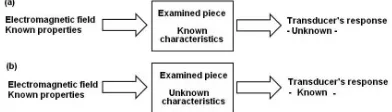
fact, the eddy current examination operation can be schematically represented (see Fig. 1).

The situation presented in Fig. 1a is named the forward problem for eddy current examination. This is frequently implemented due to two reasons:

• Facilitate the interpretation of the eddy current control’s results, no need of a lot of test pieces in which many types of defects shall be practiced.

• Allows the optimization of eddy current transducers for certain geometries, material properties and flaws possible to appear in the materials to be tested.

Fig. 1. General presentation of electromagnetic examinations, a) forward problem, b) inverse

problem

The situation presented in Fig. 1b is named the inverse problem for eddy current examination. Solving it allows the quantitative evaluation of emphasized flaws.

The electromagnetic field applied to the examined piece can be:

• harmonic

E r t E r e H r t H r e

j t j t , , ,

( )

=

( )

( )

=

( )

0 0 ω ω (1)

where r is the position vector, j= −1, ω is the angular frequency, E₀ and H₀ are the amplitudes of electrical and respective magnetic fields.

This case is known as mono-frequency examination and is extremely researched and utilized [8] and [9].

• a source of harmonic components with angular frequencies ω1, ω2, ...

E r t E r e E r e H r t H r e H r e

j t j t

j t j

, ... ,

,

( )

=

( )

+

( )

+

( )

=

( )

+

( )

1 1 2 2

1 1 2

ω ω

ω ωω₂t_+.... (2)

This eddy current examination method is named multi-frequency technique [9] with different shapes of impulses.

The real term from Eq. (9) represents the attenuation constant of the field in the conductive material and the imaginary term represents the phase constant, both being equal in modulus.

We can define the standard penetration depth as:

δ

ωµσ

= 2 , (10)

and represents the distance at which the amplitude of field is e times attenuated (e is the natural logarithm basis).

The detection of flaws, or anomalies, by

means of eddy current depends upon the fact that

flaws are not electrically conducting and that the eddy current flow is interrupted at the boundary of the flaw. The flaw, therefore, can be considered

to be an inhomogeneity, which consists of conductivity, σt , is known a priori.

The electric permittivity and magnetic permeability of each region are those of free space,

ε0, and µ0. Hence, the first two Maxwell equations

for the two regions are:

known region ∇× = −

∇× =

(

+

)

E j H

H j E

0 0 0

0 0 0 0

ωµ

σ ωε

,

, (11)

flawed region ∇× = −

∇× =

(

+

)

E j H

H j E

f f

f f f

ωµ

σ ωε

0

0 .

(12)

Upon subtracting (12) from (11), we get:

∇×

(

−

)

= −

(

−

)

∇×

(

−

)

=

(

−

)

+

+

(

−

)

+

E E j H H

H H E E

j E E

f f

f f

f

0 0 0

0 0 0

0 0 0

ωµ σ

ωε σ

,

−−

(

σ_f

)

E_f, (13)

where we have added and subtracted σ₀Ef to get

the final form.

Thus, the perturbation of the

electromagnetic field E0−Ef, H0−Hf satisfy

the same equation as the original electromagnetic

field within the known region, except for the presence of the anomalous region, or flaw. This

term, which is equivalent to a current source, Ja

, represents the presence of the anomalous region,

or flaw. It is important to note that Ja vanishes off

at the flaw, because there σt= σ0.

In the usual way a vector wave equation for E0−Ef can be derived from Eq. (13):

∇×∇×

(

−

)

= − ∇×

(

−

)

=

=

(

−

)

(

−

)

−

− −

E E j H H

j E E

j

f f

f

0 0 0

2

0 0 0 0

0 0 ωµ

ω µε ωµ σ ωµ σ

(

σσ_f

)

E_f.

(14)

Eq. (14) can be considered as a fundamental equation of eddy current nondestructive testing and, in principle, can be solved through two procedures:

• analytical,

• numerical.

From the analytical procedures, the Green’s function method [11] and [12] will be presented and from the numerical ones, the finite element method [13] will also be presented.

2 ANALYTICAL SOLVING OF FORWARD PROBLEM USING DYADIC GREEN’S

FUNCTIONS METHOD

The dyadic Green’s function establishes a bi-univocity relationship between a current source with J r( ') density and the field E r( ) created by this source in the observation point r:

E r G r r J r dr

Vsource

( )

=

_∫



(

, '

) ( )

' ', (15)

where the integral extends on the source volume and G r r( , ') is the dyadic Green’s function.

Analyzing Eq. (14) it can be observed that the last term from the right member can be

considered as a source that extends on the flaw

volume and thus it can be write immediately as a

formal solution of Eq. (14) for the perturbed field E0−Ef:

E r E r_f j G r r E r dr

V flaw f f

0( )− ( )= ωµ0

∫

( ) ( )

(

σ0−σ

)



, ' ' '. (16)

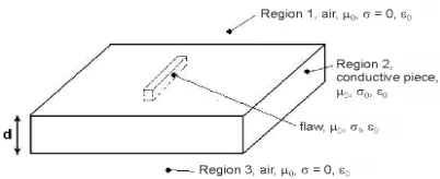
Let us consider a simple planar geometry to can exemplify the method. This is presented in Fig. 2.

The geometry of the problem allows the decomposition of the space in three regions:

• region 1, free space over the piece,

• region 2, the conductive piece,

• region 3, free space under the piece.

The following notations will be introduced:

• for the dyadic Green’s functions G r rij

(

, '

)

the field produced in the point r from region

i, due to a point source r' placed into region

j, with i, j = 1,2,3,

• for the electrical fields E_{1 2,}

( )

r the electrical field in region 1 or 2 with flaw present; E r0( ) the incident electrical field.

Eq. (16) allows the calculation of E in the zone of flaw (region 2):

E r E r j G r r E r dr

V flaw

f

0 1 0 0 12 2

0 1 ( )− ( )= ( ) ( ) −      ∫ ωµ σ σ σ 

, ' ' '. (17)

An integral equation that allows the calculation of perturbed electric field in region 1 where both the source of electric field and the device for measurement of the field are placed is disposed at the same time.

E r E r j G r r E r dr

V flaw

f

0 1 0 0 12 2

0 1 ( )− ( )= ( ) ( ) −      ∫ ωµ σ σ σ 

, ' ' '. (18)

If we consider that the incident electrical

field E r₀

( )

is produced, for example, by a coil through which an alternative electrical current with J r0

( )

' density circulates.

E r j G r r J r dr

Vexciting coil

0( )= ωµ π02

∫∫

21( ) ( )0 

, ' ' '.

_

(19)

Introducing Eq. (19) in Eq. (18), the electric

field E r₁

( )

due to the presence of flaw in region 2

can be calculated.

The integral equations which result are Fredholm equation, 2nd _{range that has not exact}

solutions. From this reason, a discretization procedure shall be used, allowing in the same time the transformation of Fredholm integral equation into a system of algebraic equations. The one most frequently used is represented by the method of moments [14] and [15].

To apply this method, a mesh is applied over the interest zone of the piece presented in Fig. 2 (the zone containing the flaw). The cells must be small enough, so that the field in the interior of

the mesh cells might be considered equal with the field in the center of the cell.

Decomposing E r₂

( )

and σ_σf

0 1 −       after

base function:

E r E r P r

P r j j Nc j f j j j Nc 2 1 0 1 1

( )

=

( ) ( )

− =

( )

= =

∑

∑

, , σ σ σ (20)

where P rj

( )

are basis functions that can be chosen

in different ways [15] and Nc is the number of cells

from mesh.

Replacing Eq. (20) in Eq. (17), finally the

following is obtained:

E r P r j E r

G r r P r

j j Nc

j j j

j Nc V flaw j

( ) ( )

+

( )

⋅ ⋅

(

)

= =

∑

∑

∫

1 0 0 1

22

ωµ σ σ



, '

(( )

' dr E r′ = 0

_{( )}

' .

(21)

Taking the moments of Eq. (21), meaning the multiplying of Eq. (21) with weighting functions Q ri

( )

, i = 1, 2, ..., Nc and integrating

over the flaw:

E r P r Q r d r

E r j dr G

j j Nc j i V flaw j j Nc j

( )

( ) ( ) ( )

+ +

( )

= =

∑

∫

∑

1

1 0 0 22

σ ωµ σ  VV flaw V flaw j i V flaw i r r

P r dr Q r dr E r Q r dr

∫

∫

∫

(

)

⋅ ⋅

( )

( )

=

( ) ( )

, '

' ' ' ₀ ,

ii 1 2 N = , ,.., c .

(22)

The vector matrix version of Eq. (22) is:

A j+ G E F

(

ωµ σ_{0 0}

)

= , (23) where the two supralines means matrix.

Aij Q r P r dri

flaw j

=

∫

( ) ( )

, ₍₂₄₎

G_{ij j} Q r dr_i G r r P r dr

V flaw V flaw j

=σ

_∫

( )

_∫

₂₂

₍

, ′

_{) ( )}

' ', (25)

Fi E r Q r dr

V flaw

If the bases function P r_j

( )

re chosen as pulse function:

P r r cell j

otherwise

j

( )

= ∈    1

0 (27)

and weight function Q ri

( )

as delta function:

Q r r

r

i

( )

=

( )

δ

. (28)

The variant of the method of moments used above is named point matching.

3 SOLVING OF FORWARD PROBLEM USING FINITE ELEMENT METHOD

The finite element method attempts to approximate the continuous problem in a rather straightforward way. The steps involved are the following [13]:

• Discretization: the solution space is discretized into finite elements. Finite elements are either linear, surfaces or volumes. The symmetry properties can be utilized for reducing the number of elements.

• Approximation: an approximation over a finite element is defined and has some required properties.

• Minimization: a method of minimizing the error due to the discretization must be included.

• Solution: the previous steps result in a system of equations (linear or nonlinear) which must be solved.

• Post processing of data may be required, depending on the function calculated in the previous step.

The finite element method (FEM) approximates the solution rather than the partial derivates in the differential equation. It is a volumetric method in which the approximation is valid at any point in the solution domain, not only at discrete points. The process calls for discretization of the continuum into any number of finite volumes subspaces over which the approximation is valid. These subspaces or finite elements are of any well-defined geometrical shape while the approximation is normally a polynomial interpolated over a finite number of points that define the shape of the finite element. Since the restriction on their shape and

size are minimal, finite elements are well suited for discretization of awkward geometries. The elements may not be uniformly distributed and can be of any size. Furthermore, it is possible to mix different types of elements to increase the FEM ability to handle a given geometry.

A number of commercial finite element and volume integral codes capable of simulating arbitrary shaped defects and tests geometries are currently available. An interesting variation of the FEM that relies on the underlying mesh and element mode connectivity is the class of meshless methods which dicretizes the domain by a set of nodes alone [16].

One of most interesting applications involve the use of numerical models for calculating the probability of detection and the generation of receiver operating characteristics for a given set of conditions [17]. Although such probability of detection (POD) models cannot account for human factors, they are very useful for isolating physical factors that contribute to variations in test results and the impact of such models will become more commonplace as industry begins to embrace the concept of design for testability and life cycle management in the future.

Y AX= , (29)

where Y is a unicolumn vector which represents the response of the assembly eddy current transducer-equipment, X is unicolumn vector which represents the parameters of the piece’s degradation and is unknown and A is the model matrix.

The solution of the inverse problem consists in determining the vector X elements knowing the elements of Y from measurements and the matrix A due to the analytical or/and numerical modelling of the phenomena. Formally, the solution of the problem is written:

and the bigger one), so that a small variation of data can produce a completely different solution [18]. In these conditions, the matrix A must be preconditioned using different regularization algorithms.

Simulation models are increasingly being used as a basis for solving inverse problems. The most straightforward method is to use an iterative scheme where an appropriate norm of error between the output of a simulation model is used and the test signal to adjust the material parameters until agreement between the signals is obtained. A number of schemes to reduce the computational effort ranging from table look-up schemes to methods that improve the convergence rate have been proposed [19] to [21]. The principal disadvantage lies in the computational border associated with the implementation of those inversion schemes although some of the newer methods appear to be successful in overcoming this problem. These models based inversion schemes will become more popular as computational power becomes less expensive. Such inversion schemes offer the obvious advantage of not requiring any training data unlike systems based approaches which typically need substantial amounts of data. Model based inversion schemes may be the only choice in situations where training data is either scarce or not of the quality required to design robust defect characterization systems.

4 THE INVERSE PROBLEM

At the core of those presented in Fig. 1, the inverse problem consists in the evaluation of the characteristics of the physical system made from the piece to be examined which contains flaws from the knowledge about electromagnetic field applied in different points of the piece and the response of the eddy current equipment in the same points. From the physical model which has been developed (indifferent that represents analytical or numerical solutions), linearized and digitized, the eddy current control operation can be represented through a matrix equation

5 EDDY CURRENT TRANSDUCERS

The eddy current transducers must accomplish two roles:

• shall induce eddy current into the conductive material to be examined,

• shall emphasize their flow modifications due to material degradations.

The simplest method to create time variable magnetic fluxes which shall induce eddy current into the material to be examined is represented by the coils crossed by alternative currents, by current impulses or more alternative currents with different frequencies.

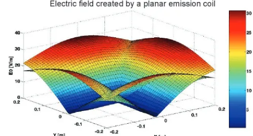
This coil is named the emission part of the eddy current transducer.

In Fig. 3 are presented, for planar geometry, few types of emission coils and the electric field created by them, at the level of examined piece. The frequency of alternative current is 100 kHz and amplitude is 0.1 A.

To emphasize the induced eddy current and the effect of material degradation over their propagation, sensors sensitive to the variation of magnetic field can be used: bobbins, sensors with Hall effect, sensors based on quantum effect – SQUID [22], sensors based on magneto-resistive effect –GMR [23].

The most utilized sensors for emphasizing eddy currents are the bobbins with and without magnetic core. Other types of sensors are less utilized due to certain limitations as frequency range that can be detected, (usually until few tens of kHz) as well as their costs, especially for SQUID.

The eddy current transducers can be:

• absolute – the signal delivered by the transducer depends by the state of the piece to be tested in the point in which the transducer was fixed,

• differential – the signal delivered by the transducer represents the difference between two neighbor region of the piece to be tested.

The simplest type of absolute eddy current transducer is represented by the transducer with a unique coil in which the same coil generates time variable magnetic field that induces eddy current in the tested piece and at the same time, due to the modification of resistance and inductive reactance emphasizes the eddy current.

The absolute transducers emphasize the material degradation on the entire surface but they have a low signal to noise ratio. In adition, they are sensible to the variation of lift-off. The differential transducers emphasize only the modifications in the profile of the degradation, they are less sensible to the lift-off and have lower signal to noise ratio.

The inventiveness in the domain of eddy current transducer is very large. Thus, the eddy

current transducer with orthogonal coils has been developed (Fig. 5a). It is made from a ferrite cup core inside which the emission coil is inserted and orthogonal on it is wounded the reception coil. The transducer is a send-receive type, absolute but is relatively less influenced by the modification of lift-off and presents good signal to noise ratio [24]. With its help, plates form carbon-epoxy composite were tested, the structure of the reinforcement Fig. 3a. Circular coil with 100 turns, inner diameter 1.8 cm, outer diameter 4 cm, height 4 mm;

Fig. 3b. Rectangular square coil with 100 turns, side of 4 cm and section of winding 4 mm;

fibers as well as the delamination due to impact were emphasized [25].

Fig. 4. Eddy current transducer for the control of tubes

In Fig. 5b the amplitude of signal delivered by the transducer at the scanning of a region from the composite plate that contains a delamination due to an impact with 4 J energy is presented.

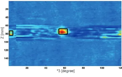
Since with the occasion of periodical outage at the nuclear power plants, the tubular bundles of steam generators are completely examined by eddy current, a special attention was accorded to the development of adequate transducers. The pancake rotating coil type transducer was developed for the confirmation of flaw indications delivered by the differential and absolute transducers that pass inside the tubes as well as for a better evaluation of the emphasized discontinuities severity. The transducer rotates around the tube’s axis with relatively high revolution speed (60 to 120 rot/min) and at the same time goes forward inside the tube (axial speed 2 to 3 mm/s). Thus, by correlation revolution speed – transducer diameter – advance speed, the entire surface of the tube can be scanned. In Fig. 6 the amplitude delivered by this type of transducer is presented. The emphasized flaws are marked in the image. In this way, the orientation of flaws can be evidenced.

The pancake rotating coil transducer type, besides the clearly advantages, presents a series of limitations as: low axial advance speed, thus an increasing of the inspection time, the existence of rotating parts and the difficulty in transmitting

the signal from the transducer to the equipment. The eddy current transducer with rotating magnetic field was developed to overtake these disadvantages [26] and [27]. The transducer is a send receiver absolute type and does not contain parts in rotation.

Fig. 5a. Eddy current transducer with orthogonal coils

Fig. 5b. The amplitude of the signal delivered by the transducer at the scanning of a region from the composite plate that contains a delamination

due to an impact with 4 J energy

F

ig. 6. The signal delivered by the pancake rotating probe

currents. Composing the phase of the fields created by the three coils, a radial rotating magnetic field is created, having the same angular frequency as of the three phased currents. The reception part of the transducer is made from a circumferential array of reception coils (Fig. 7a). The physical realization of the inner eddy current transducer with a rotating magnetic field for the inspection of pressure tubes from pressurized heavy water reactors is presented in Fig. 7b and the amplitude of the signal delivered by the reception array is presented in Fig. 7c.

Fig. 7a. Scheme of inner eddy current transducer with rotating magnetic field

Fig. 7b. Physical realization

Fig. 7c. Signal delivered by the transducer

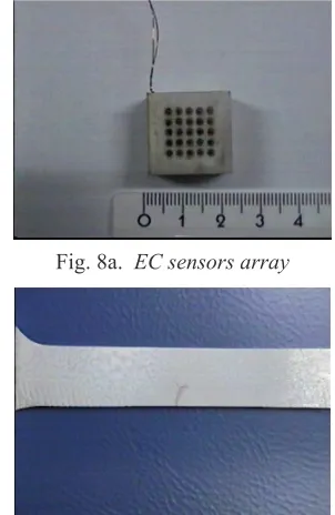
It is possible that the future of eddy current transducers will be the use of sensors array. These have started to be initially used for the increasing of the control speed [28]. Using a sensor array made from an emission coil and an array of reception coils, together with a super resolution procedure, very small discontinuities as fatigue cracks lattices have been emphasized [29] and [30].

Fig. 8a. EC sensors array

Fig. 8b. Fatigue crack lattice emphasized by penetrant liquid

Fig. 8c. Signal delivered by the EC sensors array

6 INSTRUMENTATION

The arrival of the microprocessor in the 1970s and the availability of inexpensive analog to digital (A/D) converters in recent years have had, perhaps, the most impact on instrumentation. Signals can now be routinely be sampled and quantized with 16 bit precision and as a consequence, a bulk of the processing can be performed in discrete-time. Sources of noise introduced in the signal, excluding noise introduced by the transducer, from start (transducer output) to finish (digital output of the instrument) include quantization noise, error introduced due to finite word length and algorithmic errors. The quantization noise is closely related to the number of bits associated with the A/D conversion process. A crude rule of thumb is to assume an improvement of 6 dB in the signal-to-noise ratio (SNR) for every additional bit. Quantization noise is seldom a concern these days with the ready availability of 16 bit converters in the case of conventional eddy current applications. Round-off errors due to finite word length were a matter of concern when microprocessors could not handle fast floating point calculations. The availability of relatively inexpensive 32-bit floating point digital signal processors with cycle time as low as 3.5 ns has rendered this issue moot. The overall SNR of eddy current instruments have leapfrogged as a consequence and most instruments offer performance levels that were simply not possible a few years ago. Ready access to inexpensive computational horsepower with massive amounts of storage within the instrument has also revolutionized our ability to extract and process information in numerous ways. Since most functions are now implemented in software, programmability has become a common place feature. High, low and band pass filters are routinely digital in nature. Features such as rotation, translating and gain and most importantly graphics are all implemented in software. This allows the user to tailor the instrument characteristics to the application far more effectively.

Prognostication in a rapidly changing world is very difficult. However, it is easy to see that spectacular improvements with respect to computation speed and memory will continue to

have an impact on the industry. It is more than likely that this will affect the way in which the inspection data is interpreted. Current industrial practice is to rely either on manual interpretation or simple calibration based approaches to estimate the size, shape and location of the flaw. Access to vast amounts of computation power would allow instrument manufacturers to incorporate sophisticated signal interpretation algorithms. A number of three-dimensional defect characterization approaches, both model and system based, have been proposed in recent years. It is relatively safe to assume that such defect characterization algorithms would become an integral part of the instrument menu. In the case of specific geometries, it may even be possible to use the defect profile estimate to calculate its impact on the structural integrity of the test component within the instrument. In short, we will very likely see the migration of activities that have hitherto been performed off-line to the eddy current instrument. The ease with which application specific integrated circuits (ASIC) can be designed and manufactured today as well the emphasis on miniaturization will inevitably result in smaller instrument footprints. The limitation is, of course, the size of the display required to present large amounts of information. This is being addressed through the use of head mounted displays. Such displays are also likely to become commonplace for displaying data in a virtual reality environment. In the future it should routinely be possible to “navigate” through a virtual world allowing the user to examine a defect profile estimate in 3D from any arbitrary perspective using a stereoscopic head display.

The availability of high resolution (18 bits and higher) A/D converters will have an impact on pulsed eddy current and remote field eddy current methods. These inspection methods will be able to make use of the large dynamic range and low noise floor of such converters. The circuits preceding the A/D converter (such as the anti-aliasing filter) in the processing scheme will have to be designed very carefully, of course, to ensure full exploitation of their low noise characteristics.

7 SIGNAL PROCESSING

Signal processing techniques represent a powerful approach for improving the probability of detection. Such techniques are also very often used to enhance the quality of the signal by reducing noise and other artefacts that detract from our ability to detect and characterize the flaw. Signal enhancement procedures are of interest in situations where the signal is interpreted manually as well as in case where it is analyzed using an automatic system.

Signal quality can be enhanced in a variety of ways ranging from simple filtering schemes to those that adapt with noise statistics. The latter are particularly useful when the noise is highly correlated with the signal. A number of new approaches have been proposed in recent years for the classification of defect signals. A variety of pattern recognition techniques based on statistical as well as trainable approaches have shown promise [31].

Prominent among the latter category are those that make use of neural networks. Equally interesting developments are occurring with regard to the development of systems based methods for estimating defect profiles.

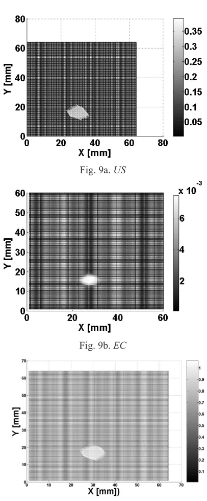
One of the more exciting developments in the field involves the concept of data fusion. The basic premise is that it is possible to garner additional information concerning the state of piece by combining information from multiple sensors. Sensors could be of the same type (operating at different positions and/or excitation frequency) or they could be entirely different from each other. Fig. 9 shows, after [32], the data fusion based on the theory of evidence between the data from ultrasound control using Lamb waves generated by hertzian contact and

the data obtained from eddy current holography at the scanning of a region from a carbon epoxy composite plate [33].

8 CONCLUSIONS

Fig. 9a. US

Fig. 9b. EC

Fig. 9c. Data fusion

field that is over a hundred years old. However, it is safe to say that some of the most exciting developments are ahead of us. A confluence of developments in the fields of electronics, computer technology, simulation tools and signal processing is contributing to the excitement and fuelling some of the most compelling advances. Technology is indeed breathing new life into the field and there is much to look forward to in this important scientific endeavour.

Now, the electromagnetic nondestructive evaluation had been transformed from “art” to an absolutely necessarily engineering science.

The actual quality requirements impose a rigorous control on the basis of quality codes (ASME), standards (EN, ASTM, etc), or, according to ISO standards, of understanding between the producers and the beneficiaries. The development of new theories, transducers, equipments and adequate analysis software will lead to an increase in the probability of detection for the highest possible reliability coefficient.

The development of new types of materials and their different applications (different classes of materials and structures in the construction of International Spatial Station, the superconductors used in ITER reactor, usage of known materials in special purposes as components of The Large Hadron Collider from CERN) made that the eddy current examination shall represent not a close domain, but, on the contrary, a dynamic domain, a fully evolving one.

9 ACKNOWLEDGEMENTS

This paper has been supported by the Romanian Ministry of Research, Development and Innovation under National Plan II Contracts: No.71-016/2007 MODIS, No.32-134/2008 SYSARR and Nucleus Program, Contract no. No.09430104

10 REFERENCES

[1] Faraday, M. (1885). Experimental researches in electricity. vols. I. and II. Richard and John Edward Taylor, vol. III. Richard Taylor and William Francis.

[2] Foucault, J.B.L. (1913). Catholic Encyclopaedia. New York: Robert Appleton Company.

[3] Shull, P.J. (2002). Nondestructive evaluation: Theory, techniques and application. Technology&Engineering, NY. [4] Cecco, V.S., Drunen, G. van, Sharp, F.L.

(1983). Eddy current manual. vol. 1, AECL 7523, rev. 1, Chalk River.

[5] Forster, F., Breitfeld, H. (1952). Theoretische und experimentelle Grundlagen der Zerstorungsfreien Werkstoffprufung mit Wirbelstromverfahren parts I und II, Z Metallkunde, vol. 43, no. 5, p. 163-180. [6] Forster, F., Breitfeld, H., Stombke, K.

(1954). Theoretische und experimentelle Grundlagen der Zerstorungsfreien Werkstoffprufung mit Wirbelstromverfahren

parts III und IV, Z Metallkunde, vol. 48, no. 5, p. 166-199, 221-226.

[7] Young, A. (2008). The Saturn V F-1 engine, powering Apollo into history. Springer, Berlin.

[8] Dood, C.V., Deeds, W.E. (1968). Analytical solutions to eddy current probe coil problems. J Appl. Phys., vol. 39, p. 2829-2838.

[9] Moore, P.O., Udpa, S.S. (2004).

Nondestructive Testing Handbook. 3rd _Ed.,

vol. 5, Electromagnetic testing, ASNT, OH. [10] Lepine, B.A., Wallace, B.P., Forsyth, D.S.,

Wyglinshi, A. (1999). Pulsed eddy current method. NDT.Net, 4,1.

[11] Tai, C.T. (1994). Dyadic green’s functions in electromagnetic theory. IEEE Press, NY [12] Chew, W.C. (1999). Waves and fields in

inhomogeneous media. Wiley-IEEE Press. [13] Ida, N. (1995). Numerical modeling for

electromagnetic nondestructive evaluation.

Chapman & Hall, London.

[14] Harrington, F. (1968). Field computation by moment methods. Mc.Millan, NY.

[15] Balanis, C.A. (1989). Advanced engineering electromagnetics. J. Wiley & Sons, NY. [16] Xuan, L., Zeng, Z., Balasubramaniam,

S., Udpa, L. (2004). Element-free Galerkin method for static and quasi-static electromagnetic field computation. IEEE

[17] Rajesh, S.N., Udpa, L., Udpa, S.S. (1993). Numerical model based approach for estimating probability of detection in nde application. IEEE Trans. on Mag., vol. 29, no. 2, p.1857-1861.

[18] Bertero, M.E., Pike, R. (1993). Signal processing for linear instrumental systems with noise, signal processing and its applications. Bose, N.K, Rao, C.R. (Eds.) North Holland, Amsterdam.

[19] Kojima, F., Okajima, N. (2001). Crack profiles identification of steam generator tubes in PWR plants using database.

Electromagnetic Nondestructive Evaluation

(V), Pavo, J. (ed.) IOS Press, p. 97-104. [20] Li, Y., Liu, G., Shanker, B.S., Sun, Y.,

Sacks, P., Udpa, L., Udpa, S.S. (2001). An adjoint equation based method for 3D eddy current signal inversion electromagnetic nondestructive evaluation. (V), Pavo, J. (Ed.), IOS Press, p. 89-96.

[21] Grimberg, R., Udpa, L., Udpa, S.S. (2008). Electromagnetic transducer for the determination of soil condition. International Journal of Applied Electromagnetics and Mechanics, vol. 28, no. 1-2, p. 201-210. [22] Pandney, W. (1998). Response function of

an electromagnetic microscope. Review of Progress in QNDE, Thompson, D.O., Chimenti, E.E. (Eds.), 17, Plenum Press, NY, p. 1025-1031.

[23] Danghton, J., Braun, J., Chen, E. (1994). Magnetic field sensors using GMR multilayer. IEEE Trans. on Magnetics, vol. 30, no. 6, p. 4608-4610.

[24] Savin, A., Grimberg, R., Mihalache, O. (1997). Analytical solutions describing the operation of rotating magnetic field transducer. IEEE Trans. on Magnetics, vol. 33, no. 1, p. 697-702.

[25] Grimberg, R., Savin, A., Steigmann, R., Bruma, A., Barsanescu, P. (2009). Ultrasound and eddy current data fusion for evaluation of carbon epoxy composite

delaminations. INSIGHT, vol. 51, no. 1, p. 25-32.

[26] Grimberg, R., Udpa, L., Savin, A., Steigmann, R., Udpa, S.S. (2005). Inner-eddy-current transducer with rotating magnetic field: theoretical model, forward problem. Research in Nodestructive Evaluation, vol. 16, no. 2, p. 65-77.

[27] Grimberg, R., Udpa, L., Savin, A., Steigmann, R., Udpa, S.S. (2005). Inner-eddy-current transducer with rotating magnetic field, experimental results: application to nondestructive examination of pressure tubes in PHWR nuclear power plants. Research in Nodestructive Evaluation, vol. 16, no. 2, p. 79-100.

[28] Mook, G., Michel, F., Simonin, J. (2008). Electromagnetic imaging using probe arrays.

17th _{World Conference on Nondestructive}

Testing, Shanghai.

[29] Grimberg, R., Wooh, S.C., Savin, A., Steigmann, R., Prémel, D. (2002). Linear Eddy-Current Array Transducer. INSIGHT, vol. 44, no. 5, p. 289-293.

[30] Grimberg, R., Udpa, L., Savin, A., Steigmann, R., Palihovici, V., Udpa, S.S. (2006). 2D eddy current sensor array. NDT & E International, vol. 39, no. 4, p. 264-271. [31] Udpa, L., Udpa, S.S. (1996). Application of

signal processing and pattern recognition techniques to inverse problems in NDE. Int. J. of Appl. Electromagnetics and Mechanics, vol. 9, no. 1, p. 1-20.

[32] Grimberg, R., Steigmann, R., Leitoiu, S., Andreescu, A., Savin, A. (2008). Ultrasound and eddy current data fusion evaluation of carbon – epoxy composites delaminations.

Emerging Technologies in Nondestructive Testing, Busse, G. et al. (eds.), p. 349-355. [33] Grimberg, R., Prémel, D., Savin, A., Bihan,