Optimal Control for Descriptor Systems: Tracking Problem (RESEARCH NOTE)

RESEARCH NOTE

OPTIMAL CONTROL FOR DESCRIPTOR SYSTEMS:

TRACKING PROBLEM

M. Shafiee

Department of Electrical Engineering, Amirkabir University of Technology Tehran, Iran, [email protected]

(Received: April 18, 1999 - Accepted in Revised Form: May 4, 2000)

Singu lar systems have been studied extensively during the last two decades du e to

Abstract

their many practical applications. Such systems possess numerous properties not shared by the well-known state variable systems. This paper considers the linear tracking problem for the continuous-time singular systems. The Hamilton-Jacobi theory is used in order to compute the opt imal contr ol an d associat ed tr ajectory. Two m ethod s are presented for solving th ese trajectories. The first method uses the concept of the Drazin inverse, and the second involves the derivation and solu tion of a R iccati equation. Similar to the linear regu lator problem, necessary and sufficient conditions for existence and uniqueness of a solution are stated.

Optimal Control, Riccati Equation, Singular Systems

Key Words

|A±i /k¯A³T o£ nAo |Bi ³]±U jn±« o¼iA ·µj °j nj ¼ñU ºB´ªTv¼w ,¬A°Ao ºBµjoMnB ¥¼§j ³M

²k¼ña

ºAoÇM » Çi K¼ íÇU ·§Fv« ,³§B Ç« ǽA nj /SwA R°B TÇ« ¼ÇñU o¼Ç ºB´ªTv¼Çw |A±i BM B´ªTv¼w ³¯±£ ½A ° ³®¼´ÇM ºj°n° ³LwBdÇ« ºAoM »M± @B]-¬±T¦¼ªµ ·½o ¯ pA /SwA ³T o£ nAo ³]±U jn±« ¼ñU ³Tw±¼Q ºB´ªTv¼w ³§jBí« ¬jn°C SwkM (J) ° ½q½njt±ñí« ³LwBd« ( §A) x°n °j ³M nB ½A /j±{»« ²jB TwA ³TvMA° ºB´T§Be ²kÇ{ ³ÄAnA ¬C ¬j±M BTñ½ ° JA±] j±]° ºAoM » B ° ¨p¿ ½Ao{ ,n±U¿±£n ³§Fv« ³M ³¼L{ /j±{»« ¨B\¯A »UBñ½n /SwA

INTRODUCTION

Consider the system of the form:

(1) x(t

Ü) = xÜ

E X³(t) = A x(t) + B u(t)

where E, A and B are constant matrices. If

¼

E

¼

= 0 then the system described by Equation 1 is called a singular system [1], degenerate system [2], ge n e r a lize d st a t e sp a ce syst e m [3], descriptor system [4], or semi-state system [5]. Syst e ms which sa tisfy t he se p rope rt ie s can consist of both static and dynamic equations and ne e d not be causal. The se type s of syste ms appear in many pract ical applicat ions such as robotics, optimal control, electrical networks, economics, large scale interconnected systems, biology, power syste ms, neural delay systems, and aircraft dynamics with algebraic constraints.

It has taken considerable effort to extend the theories available for state variables to singular s ys t e m s . T h e p r o b l e m o f d e r i vi n g a cont inuous-time singular syst e m from some initial st at e to a de sired final stat e has bee n discusse d in [1,2,7,8]. In [9,10,24] t he pole place me nt of t he singular syst e ms has be e n investigated. In the area of optimal control, the line ar singular re gulat or proble m has be e n considered in [11,12] for the discrete-time case and in [2,6,13-19] for the continuous-time case. By using state feedback, the generalized Riccati e q u a t i o n fo r b o t h t i m e - in va r ia n t a n d time-varying cases has been obtained [20,21]. It

wa s sh own t ha t fo r t h e case

¼

R

¼ Ú

0, t he

R iccati equation is symme tric (where R is the conventional quadratic weighting matrix), but

symmetric. Necessary and sufficient conditions for the existence and uniqueness of a solution have also been derived.

Our goal in this paper is to take some steps t o war ds ge ne r alizat ion o f lin e ar r e gu lat or problem, namely linear tracking problem for singular systems. In t his case, we wish to find the control that cause s the out put to t rack a

desired output state,

G

(t). For this, we wish to

find the control which minimizes a performance in d e x, J . I n se ct io n I I we de scr ib e t h e formulation of the linear tracking problem for t h e sin gu la r syst e m s. I n a d d it i o n , t h e H amilton-Jacobi theory is applie d in order to compute t he optimal control and associate d trajectory. Section III is devoted to the solution of t hese traje ctories by two me thods (namely direct and R iccati approaches). The condition for exist ence and uniquene ss of a solution is also given.

FORMULATION OF THE PROBLEM

In this section, we extend the results obtained for t he line ar re gu lat or proble m [6] to the tracking problem; that is, the desired value of the state vector is not the origin. Given that:

E x0(t) = A x(t) + B u(t) + w(t)

(2a) z(t) = C x(t)

where w( t ) is a de terministic input or plant

noise , t he mat rix E is singular , wit h x

e

Rn,

u

e

Rm, w

e

Rn, z

e

Rn. Additionally, we assume

t h a t t h e ma t r ix ( sE -A ) h a s a n o n -ze r o d e t e r m in a n t fo r so m e va lu e o f s. T h is conditions, ensures that for appropriate initial conditions, E quation 2a posse sse s a unique solution [1] (namely it is tractable).

We wish to find the control which minimises the performance index,

J = __ [1

G

(t_f) - z(t_f)]T ET SE[

G

(t_f) - z(t_f)] + __

2

1 2 (2b)

ß

tf[

´ G

(t) - z(t)

´

2+

´

u(t)

´

2_R] dt

@@

Q t

Ü

where

G

(t) is the desired output state vector. S,

Q , R ar e symme t ric mat r ice s an d at le ast

positive semi-definite (p.s.d.). The final time t_fis

fixed, x(t_f) is free and the states and controls are

not bounded. The Hamilton is as follows:

H[x(t), u(t),

l

(t), t] = __1

´ G

(t) - Z(t)

´

2 + __

2

1 2

Q

(3)

´

u(t)

´

2 +

l

T(t) [Ax(t) + Bu(t) + w(t)]

@

R

By u sin g t h e calcu lu s o f va r iat io n a n d following the same approach as we did for the regulator problem [6], we obtain:

J = __ [

G

(t

f) - z(tf)]

T

ET SE[

G

(t

f) - z(tf)] + __

1 2

1 2

ß

tf

´ G

(t) - z(t)

´

2+

´

u(t)

´

2+

l

T(t) [Ax(t)

@@

R

@

Q

@@

t Ü

(4)

+ Bu(t) + w(t) - ExÜ(t)] dt

W it h so m e ma n ip u la t io n we h a ve t h e following:

(5a)

BT

l

(t) + Ru(t) = 0

___ = 0

Ã

H

Ã

u

ET

l

Ü(t) = - CT QCx(t)

-- ___ = E

Ã

H T

l

Ü(t)

Ã

x

(5b)

AT

l

(t) + CT Q

G

(t)

ExÜ(t) = Ax(t) + Bu(t) +

___ = Ex

Ã

H Ü_(t)

Ãl

(5c) w(t) or

Þ

B 0

Þ £

A

0

Þ £

xÜ(t)

£

E 0

¤

¤

@

¤

¤ ¤

¤

¤

¤

=

¤

- CT QC -AT 0

0

¤ ¤ l

Ü(t)

ET

¤

0

¤

¤

@

¤

¤ ¤

¤

ø

R -BT 0

ø

@

¥

0

ø ¥

uÜ(t)

0

¥

0

Þ

0 0

@

£

1

Þ

£

x(t)

Þ

£

w(t)

¤

@

¤

¤

¤

(5)

¤

¤

0

¤

CT Q

¤

+

¤

0

¤ l

(t)

ø

¥G

(t)

¤

¤ ¤

¤

ø

0 0 0

@

¥

ø

¥

u(t)

With the initial and terminal condition, x(t

Ü) = xÜ,

l

(tf) = C

T

ET SE [Cx(t

f)

-(6) F(t

f)]

SOLUTIONS

solved by two methods.

Assuming

¼

R

Method 1 (direct approach)

-¼ Ú

0, we find t h at u ( t ) = -R-1BT

l

( t ). By

su bst it u t in g fo r u( t ) in ( 5) , we o b t a in t h e following:

Þ

-BR-1BT

A

£

Þ £

xÜ(t)

Þ

0

£

E

¤

¤

¤

¤ ¤

¤

¤

¤

=

¤

¤ ¤

¤

ø

- AT

¥

- CTQC

ET

ø ¥l

Ü(t)

ø

¥

0

Þ

Þ£

w(t) 0

£

1

Þ

£

x(t)

¤

¤¤

¤

¤

¤

(7a)

¤

¤¤

¤

+

¤

¤

ø

ø¥ G

(t)

CT Q

¥

0

ø

¥ l

(t)

Comparing with the regulator problem, we also have a for cing pa rt whe r e as we had a homogeneous equation in the pre vious case. The above equation can be written as follows:

(7b)

E X0 (t) = A X (t) + B f(t).

A ssu min g t h e fu n ct io n f( t ) is k-t ime s continuously differentiable around initial time, t

0 we can st ate t he ne ce ssary and sufficie nt

conditions for the existence and uniqueness of solution for tracking proble m in t erms of t he solution of original singular syst e m. Be ing k-times differentiable is due to the solution of the singular system which is:

@

D

@

D

@

D

@

^^

@

^

@

^ ^^

x(t) = eE A

@

(t-tÜ) E A x(t - t₀) + eE A(t)

D

^

@

^

t_^^

@ @

^

@

^

ß

eE A(S) E B f(s) ds - (I - E ED)

t Ü

D

@@@

D k-1

@

^

@

^

@@

^

@

^ ₍₈₎

S (E A)i A B f

@

i(t)

i=0

where

(^ ) = (

l

E - A)-1 (.) for some

l

, k is the index

of Matrix E, (.)D is the Drazin inverse and fi(t)

refers to the ith derivative.

A s s u m i n g f ( t ) i s k - t i m e s

Theorem 1

-continuously diffe re ntiable around t0, wit h

c o n s i s t e n t i n i t i a l c o n d i t i o n , t h e

non-homoge neous E quation 7b is tractable (regular) iff the original singular E quation 1 is tractable.

By some manipulation we can e asily

Proof

-obtain:

§

§

§

BR-1BT

§

sE-A

§

§

§

=

§

(sE+A) T

§

§

§

§

§

@@@@

sET+AT

§

CTQ C

§

§

§

sE-A

§

.

§

I - BR-1BT (sE+A) -T CT Q C

(9)

(sE-A)-1

§

For simplicity let us write the above equation as follows:

D

=

D

₁

D

₂

D

₃

It is easily seen that

DÚ

0 (by

Only if Part

-[1] it means Equation 7b has a unique solution)

implies

D

₁

Ú

0, (that is Equation 1 has a unique

solution).

D

₁

Ú

0, imp lie s

D

₂

Ú

0, an d since

If Part

-D

₃

Ú

0, therefore

DÚ

0, which gives the result.

For the case

¼

R

¼

= 0 we cannot

Remark 1

-find u dir e ctly fr om E quat ion 5a. Thus we should solve the non-homogeneous Equation 5 directly as a singular system (see [1]).

Method 2 (Riccati approach)

-For deriving R iccati

¼

R

¼Ú

0:

Case 1

-equation we assume

(10)

l

(t) = P(t) Ex(t) - L(t)

Then

(11)

l

Ü(t) = PÜ(t) Ex(t) + P(t) ExÜ(t) - LÜ(t)

and

ET

l

Ü(t) =E T PÜ(t) Ex(t) + ET P(t) ExÜ(t) - ET

(12)

LÜ(t)

By a procedure similar to that of the singular re gulat or problem, we obt ain t he following equation:

E + ET P(t) BR-1 BT P(t) E] x(t) +

[ET P(t) BR-1BT L(t) + ET P(t) w(t) - ET LÜ(t)

(13)

- AT L(t) - CT Q

G

(t)] = 0

Since Equation 13 holds for all non-zero x(t), the term premult iplying x(t) and second term must be zero. Therefore, we have the following two sets of equations:

ET PÜ(t) E + ET P(t) A + AT P(t) E - ET P(t)

BR-1 BT P(t) E + CT Q C = 0

(14)

P(t_f) E = CT ET SEC

and

ET LÜ(t) + AT L(t) - ET p(t) BR-1 BTL(t) - ET

P(t) w(t) + CT Q

G

(t) = 0

(15) L(t

f) = C

T

ET SE

G

(t

f)

Thus, we need to solve a generalized Riccati E quation 14 for p(t) and singular E quation 15

for L(t) in order to compute

l

(t). The optimum

control law is obtained from Equations 5a and 10. That is, we have:

u(t) = -R-1BT

l

(t) = -R-1BT[P(t) Ex(t) - L(t)].

In [6] different methods for solving similar R icca t i e qu a t io n s h a ve be e n sh o wn a n d necessary and sufficient conditions for existence and uniqueness of a solution have been stated, so details of the derivation are omitted.

T h e R icca t i E qu a t io n 14 is

Theorem 2

-regular iff the system Equation 1 is -regular.

T h e r e su lt i s a n a l o go u s t o t h e

Proof

-derivation of the regulator case in [6].

Th e syst e m E q u a t io n 2 ha s a

Theorem 3

-un ique solu t io n if t he ge n e r alize d R icca t i E quation 14 and the singular system E quation 15 are regular.

H a vin g R icca t i E qu a t io n 14 a n d

Proof

-E quation 15 regular we can calculate P(t) and L(t). Therefore:

u(t) = -R-1 BT [P(t) Ex(t) - L(t)]

can be considered.

Given the singular system described

Example

-by

£

0

Þ

£

-1 1

Þ

£

1 0

Þ

¤

¤

xÜ(t) =

¤

¤

x(t) +

¤

¤

u(t)

¥

1

ø

¥

@@

0 -2

ø

¥

0 0

ø

z(t) = [1 0] x(t)

we would like to minimize the cost function

Þ

Þ

T

£

¤

£

¤

¤G

(t

f) - z(tf) E

T _SE

¤G

(t

f) - z(tf)

J = __1

2

¥

ø

¥

ø

Þ

£

t

¤

¤

@

´ G

_{(t) - z(t)}

´

2 _dt

+

´

u(t)

´

2

+ __1

ß

f

2 0

¥

@

q r

ø

where q and r are scalars. For the case S=0, we will have the following.

We first use E quation 14 to obtain R iccati equation for the above system. So we have

@@

2

@@@@

p₁₁(t_f) = 0

pÜ₁₁(t) - 2p₁₁(t) - _____ + q = 0p12(t)

r

p₁₂(t_f) = 0

p₁₁(t) - 2p₁₂(t) = 0

If we allowt_fto become infinite (t_f=

È

), we

obtain the following solutions

p

11 = 4r 1 + __ - 4r

q 4r

p

12 = __ p11

1 2

p

11 p12

Þ

@@@@

£

¤

where P =

@@@@

¤

¤

¤

ø

@@@@

¥

p

12 p22

Now, we use Equation 15 to obtain L(t). Thus

@@

Ü

l₁(t) - l₁(t) - ___p12 l₂(t) + q

G

(t) = 0

r

l₁(t) - 2l₂(t) = 0

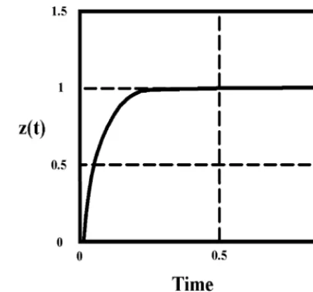
Figure 1. Optimal control.

1

l₁(t) =

ººººº

q

G

(t)

1 + _____p12

2 r

l

2(t) = __ l1(t)

1 2

l 1(t)

Þ

@@@@

£

¤

¤

where L(t) =

¤

@@@@

¤

ø

@@@@

¥

l 2(t)

After de termining P and L(t ), the optimal control will be as following:

Þ

0

£

1

Þ

T

£

0

¤

¤

¤

¤

(

_{P x(t) - L(t)}

)

u(t) = - __1

r

¤

¥

1

¤

ø

¤

¥

0 0

¤

ø

We first consider

G

(t) to be a step function.

1

-Figures 1 and 2 show the optimal control and corresponding output where r= 1 and q= 1000 and x(0)=0.

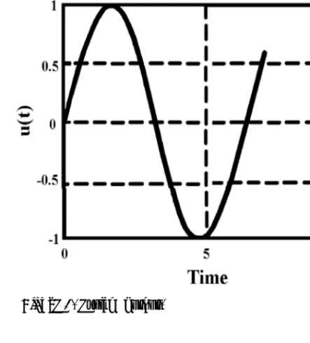
Now, consider

G

(t) be a sinusoidal function.

2

-Figures 3 and 4 show the optimal control and corresponding output for r=1 and q=10, which in this case , t he out put o f syst e m doe s not fo llow t he de sir e d t ra je ct o ry. H o we ve r by choosing r= 0.1 and q= 1000, the output follow the desired trajectory. Figures 5 and 6 show the optimal control and associated output for this choice.

Th e syst e m E q u a t io n 2 ha s a

Lemma 1

-Figure 2. System output.

Figure 3. Optimal control.

Figure 5. Optimal control.

unique solution if singular systems 1, and 15 are regular.

Combining theorems 2 and 3 gives the

Proof

-result.

A ssumin g t he ma t r ix P is con st an t , t h e following theorem is immediate.

System Equation 15 has a unique

Theorem 4

-solution iff there exists a scalar s such that the following matrix is invertible:

(16)

(sET + AT - ET PBR-1BT)

By [1], E qu at io n 15 h a s a u n iqu e

Proof

-solu t io n su bje ct t o an a pp r op r iat e in it ia l

condition ( re gular) if

¼

sET + AT - ET PBR-1

BT

¼Ú

0.

Case 2 -

¼

R

¼

= 0

In this case we cannot find u(t) in terms of

l

(t).

H o we ve r, simila r t o t h e re gu la t o r case by choosing:

(17)

u(t) = P₁

l

(t) + P₂ x(t)

and subst ituting for u in processes of deriving R iccat i e quat io n, we o bt ain t he follo wing non-symmetric generalized R iccati and singular equations respectively.

Figure 6. System output.

ET PÜ(t) E + ET P(t) A + AT p(t) E + ET P(t)

BP₁ P(t) E + ET P(t) BP₂+ CT Q C = 0

(18) and

ET LÜ(t) + AT L(t) + ET P(t) BP

1L(t) + C

T _Q

(19)

G

(t) - ET P(t) w(t) = 0

The solution of the above e quat ions can be f o u n d i n [ 6] a n d [ 1] f o l lo wi n g so m e simplifications.

Conside r matrix E as const ant.

Remark 2

-All derivations in this paper could hold for time varying case s. H owe ve r, if mat rix E is t ime varying, we have some modification as follows

for the case

¼

R

¼Ú

0.

l

(t) = P(t) E(t) x(t) - L(t)

l

Ü(t) = PÜ(t) E(t) x(t) + P(t) E(t) xÜ(t) LÜ(t) +

P(t) EÜ(t) x(t)

and

ET(t)

l

Ü(t) = - CT(t) Q(t) C(t) x(t) - AT(t)

l

(t)

combining t he above equations give s us the following equations:

ET PÜ( t ) E ( t ) + ET( t ) p(t ) [A( t ) + EÜ( t )] +

[EÜ(t) + A(t)]T p(t) E(t)

-ET(t) P(t) B(t) R-1(t) BT p(t) E(t) + CT(t) Q(t)

C(t) = 0

and

ET(t) LÜ(t) + [A(t) + EÜ(t)]T L(t)

-ET(t ) P (t ) B( t) R-1(t ) BT( t) L(t) - ET(t ) P( t)

w(t) + CT(t) Q(t)

G

(t) = 0

It can easily be seen that by changing A(t) to [A(t) + E

Ü(t)] for the constant coefficient case

the ne w e quations for the time varying case have be en obtaine d. This re sult can also be achieved for the case

¼

R

¼

= 0.

Although t hese re sults have be en

Remark 3

de ve lope d for continuous syste ms, the y can easily be extended for the discrete cases as well.

CONCLUSION

The linear singular opt imal t racking problem has be en discusse d and the H amilton-Jacobi theory is used in order to compute the optimal cont rol and associat e d t raje ct ory. We have shown that t he singular tracking proble m is compose d of two parts, a singular re gulator part, and a prefilter to determine the optimal

driving function from the desired value,

G

(t), of

the syst em output. We also have obtained the ge ne ralize d R iccati e quation for both t ime invariant and time varying cases.

REFERENCES

Cam pb ell, S.L ., "Sin gu lar Syste ms of D iffe re nt ia l 1.

Equations", Pitman, London, 1980.

Pandolfi, L., "O n the R egu lator Problem for Linear 2.

Degenerate Control Systems",Journal of Optimization Theory and Applications, Vol.33, (1981), 241-154. V e r gh e se , G .C., Le vy, B.C. a n d Ka ila t h , T ., "A 3.

G eneralized State Space for Singu lar Systems",IEEE Trans. Aut. Cont., AC-26, (1981), 811-831.

Luenberger, D .G ., "Dynamic E qu ation in D escriptor 4.

F o r m ", IEEE Trans. Aut. Cont., AC-2 2, ( 197 7) , 312-321.

Dziurla, B. and Newcomb, R.W., "The Drazin Inverse 5.

and Semi-State E q u ation s",Proc. 4th Int. Symp. on Ma ths. Theory of Networks a nd Systems, D e lft , Netherlands, (1979), 283-289.

Sh afiee , M ., "LQ R P rob le m fo r Con tin u o u s-Time 6.

Descriptor Systems",Amirkabir Journal of Science and Technology, (Winter 1993), 5-9.

Cobb, D., "Controllability, Observability and Duality in 7.

Singu lar Syst ems",IEEE Trans. Aut. Cont., AC-29, (1984), 1076-1082.

Y ip , E . L . a n d Sin co ve c , R . F ., "So lva b ilit y, 8.

Co n t r o lla b ilit y a n d O b se r va b ilit y of Co n t in u o u s D escriptor Systems",IEEE Trans. Aut. Cont., AC-26, (1981), 702-707.

J o n e s, E .R .L I , P u gh , A .C ., a n d H a yt o n , G .E ., 9.

"N e ce ssa r y Co n d it io n s fo r t h e G e n e r a lize d P o le Placement Problem Via Constant Ou tput Feedback",

Int. J. Control, Vol. 51, (1990), 771-784.

10. Fletcher, L.R ., "Pole Assignment and Controllability Su bspaces in Descriptor Systems",Int. J. Control, Vol. 66, (1997), 677-709.

11. Luenberger, D.G., "Time-invariant Descriptor Systems, Automatica", Vol.14, (1978), 473-480.

12. Mantas, G.P. and Krikelis, N.J., "L-Q Optimal Control for Discrete Descriptor System with a Complete Set of Boundary Information", Int. J. Control, Vol.47, (1988), 1467-1477.

13. Shafiee, M. and Karimaghai, P., "Optimal Control for Singu lar Systems (R ectangular Case)",Proc. of ICEE 97, Tehran, Iran, (1997), 4, 152-160 (in Persian). 14. Cobb, D ., "Descriptor Variable Systems and Optimal

St ate R egu lat ion ",IEEE Trans. Aut. Cont., AC-28, (1983), 601-611.

15. Lewis, F.L., "A Su r vey of Linear Singu lar Systems, Circuits, Syst. & Signal Processing", (1986), 3-36. 16. Bender, D.J. and Lau b, A.J., "The Linear Q uadratic

O p tim al R egu lat or for D escript or System s",IEEE Trans. Aut. Cont., AC-32, (1987), 672-688.

Control, Vol.44, (1986), 613-624.

18. W u , H .S., "G e n e ra lize d M a xim u m P r in cip le fo r Optimal Control of Generalized State-Space Systems",

Int. J. Control, Vol.47, (1988), 373-380.

19. Ka wa m o t o , A., Ka t a ya m a , T ., "Th e D issip a t io n Inequality and Generalized Algebraic Riccati Equation for Linear Q u adratic Control Problem of Descriptor System",Proc. of IFAC, San Francisco, USA, (1996), 103-108.

20. Sh o u lin g, H ., e t c., "So lvin g R icca t i D iffe r e n t ia l E qu ation with Multilayer Neu ral Networks",PROC. 36th IEEE Conference on Decision and Control, Vol.3, (1997), 2199-2200.

21. Ben ner , P., and Byer s, R ., "An E xa ct Line Sear ch

Met hod fo r Solving G en eralized Co ntinu ou s-T ime Algebraic R iccati E qu ations",IEEE Trans. Aut. Cont., Vol.43, (1998), 101-107.

22. Wa ng, D ., "Singu lar Mod el and D ecompo sit ion of Mobile Robot Motion", IEEE International Symposium on Control Theory and Application, (1997), 185-189. 23. Shields, D .N., "O bserver D esign and D etection for

Nonlinear Descriptor Systems",Int. J. Control, Vol. 67, (1997), 153-1680.

24. CH U , D .L., et c., "A G ener al Fra mework for St ate Feedback Pole Assignment of Singular Systems",Int. J. Control, Vol. 67, (1997), 135-152.