Distinguishing Error of Nonlinear Invariant Attacks
Subhabrata Samajder and Palash Sarkar Applied Statistics Unit
Indian Statistical Institute
203, B.T.Road, Kolkata, India - 700108. [email protected], [email protected]
October 1, 2018
Abstract
Linear cryptanalysis considers correlations between linear input and output combiners for block ciphers and stream ciphers. Daeman and Rijmen (2007) had obtained the distributions of the correlations between linear input and output combiners of uniform random functions and uniform random permutations. Our first contribution is to generalise these results to obtain the distributions of the correlations between arbitrary input and output combiners of uniform random functions and uniform random permutations. Recently, Todo et al. (2018) have proposed nonlinear invariant attacks which consider correlations between nonlinear input and output combiners for a key-alternating block cipher. In its basic form, a nonlinear invariant attack is a distinguishing attack. The second and the main contribution of this paper is to obtain precise expressions for the errors of nonlinear invariant attacks in distinguishing a key-alternating cipher from either a uniform random function or a uniform random permutation.
Keywords: correlation, uniform random function, uniform random permutation, block cipher, nonlinear invariant attack, distinguishing attack, error probability.
1
Introduction
Let S : {0,1}m → {0,1}n be a function arising in a context of symmetric key cryptography. Two important examples are the state to keystream map of a stream cipher, and the encryption function of a block cipher, for whichm=n. The goal of a distinguishing attack is to be able to distinguish a real cryptographic primitive from an idealised primitive. The idealised primitive could be a uniform random function ρfrom {0,1}m to{0,1}nor, form=n, it could be a uniform random permutationπ of{0,1}n.
A distinguishing attack based on correlation between input and output combiners proceeds as follows. Let
φ:{0,1}m→ {0,1}and ψ:{0,1}n→ {0,1} be two functions. The functionφserves as a combiner of the input of S while the function ψ serves as a combiner of the output of S. The correlation between input and output combiners is the correlation betweenφ and ψ◦S. This correlation is captured by considering the weight of the functionfS :{0,1}m→ {0,1} defined byfS(α) =φ(α)⊕ψ(S(α)). Suppose it is possible to find some property of S such that the functionfS has a nature which is different from fρ or fπ. Then such a property forms the basis of distinguishing S from eitherρ orπ.
Obtaining the nature offSrequires a considerable amount of ingenuity, and is obtained by carefully studying the overall design and the internal structure of S. On the other hand, the nature of fρ and fπ are obtained mathematically. To determine the success probability of an attack, it is important to have sufficient information about both fS and eitherfρ orfπ. In this paper, we will be concerned with properties offρ andfπ.
1 INTRODUCTION 2
Linear cryptanalysis: Distinguishing attacks based on linear cryptanalysis [7] is the classical example of the above scenario. For such an attack, the functions φ and ψ are linear functions. Linear cryptanalysis has an extensive history and has been successfully applied to both block and stream ciphers. When φand ψ are linear functions, precise distributions of the weights of fρ and fπ have been obtained by Daeman and Rijmen [4]. For the case of fπ, the distribution was earlier stated without proof in [9]. The results of [4] have formed the basis for an alternative formulation of the wrong key randomisation hypothesis in linear cryptanalysis [3] and has been followed up in later works [2, 1].
Nonlinear invariant attack: Nonlinear combiners of inputs and outputs of a key alternating cipher arise in the context of nonlinear invariant attack which has been introduced by Todo et al. [10]. Suppose n = m and
S is an r-round key alternating cipherEK :{0,1}n → {0,1}n. The crux of a nonlinear invariant attack is that there may exist an n-variable Boolean function g and a class of weak keys K such that for any plaintext P,
g(P)⊕g(EK(P)) is a constant which is independent of P. Such agis called a nonlinear invariant. The existence of nonlinear invariants and weak keys have been shown for practical block ciphers SCREAM, iSCREAM and Midori64 [10]. Nonlinear approximations have been previously studied by Herpes et al. [5] and Knudsen and Robshaw [6].
Our Contributions
This work makes two contributions.
The first contribution is to extend the results of Daemen and Rijmen [4] by considering correlation between arbitrary combiners of the input and output of uniform random functions and uniform random permutations. In other words, we allow φand ψ to be arbitrary Boolean functions and obtain the distributions of the weights of fρand fπ. For the case of a uniform random functionρ, if the output combiner ψis balanced, then we prove that this weight follows the binomial distribution; on the other hand, if the output combiner is not balanced, then we derive bounds on the probability that the weight deviates from its expected value. In the case of a uniform random permutation π, we show that the distribution of the weights off can be expressed in terms of the hypergeometric distribution.
Our approach to proving the results is different from that in [4]. The proofs in [4] are counting arguments and essentially consist of counting Boolean functions under certain restrictions. While this approach works when the input and output combiners are linear functions, we found it difficult to extend this approach for arbitrary Boolean functions. Instead we have used direct probability arguments. This yields proofs which are simple and at the same time work for arbitrary combiners.
The second and the main contribution of this work is to perform an analysis of the distinguishing error of nonlinear invariant attacks. The goal is to be able to distinguish EK from a uniform random permutation π of {0,1}n (or, from a uniform random function ρ). Suppose g is a nonlinear invariant for E
K. Further, suppose that distinct plaintextsP1, . . . , PN are used by the distinguisher. Then if K is a weak key, g(P1)⊕g(EK(P1)) =
· · ·=g(PN)⊕g(EK(PN)). To be able to construct a distinguisher it is required to determine the probability ε thatg(P1)⊕g(π(P1)) =· · ·=g(PN)⊕g(π(PN)). The distinguisher can make one-sided error and the probability of this error is preciselyε.
We consider the following more general problem. (This generalisation has been mentioned in Section 7 of [10].) Letg0 and gr be any twon-variable Boolean functions. We determine the probability thatg0(P1)⊕gr(π(P1)) =
2 CORRELATION BETWEEN INPUT AND OUTPUT COMBINERS 3
1. It turns out that the error probability considered in [10] is that of distinguishingEK from a uniform random function. The error probability of distinguishingEK from a uniform random permutation is obtained here for the first time.
2. The general form of the error probabilities are derived without any restriction on g0 and gr. When g0 and
gr are balanced functions, we prove the following two results.
(a) The error in distinguishing from a uniform random function is 1/2N−1.
(b) The error in distinguishing from a uniform random permutation is at least as large as the error in distinguishing from a uniform random function. This is a consequence of Jensen’s inequality. For moderate values of N, the error in distinguishing from a uniform random permutation is almost the same as the error in distinguishing from a uniform random function.
Structure of the Paper
In Section 2, we provide the generalisation of the results of Daemen and Rijmen which appear in [4]. Section 3 provides a background of nonlinear invariant attacks as distinguishing attacks and defines the relevant distin-guishing errors. Section 4 provides the analysis of the error in distindistin-guishing from a uniform random permutation while Section 5 provides the analysis of error in distinguishing from a uniform random permutation. Appendix B provides an alternative expression for the later error. Some computational results are provided in Section 6.
2
Correlation Between Input and Output Combiners
In this section, we consider the distribution of correlation between input and output combiners of uniform random functions and uniform random permutations. The case of uniform random function is analysed in Section 2.1 and the case of uniform random permutation is analysed in Section 2.2. Before proceeding, we introduce some basic concepts and notation.
For two binary strings α and β of the same length, α⊕β will denote a binary string obtained by bitwise XOR of α and β. An m-variable Boolean function f is a map f :{0,1}m → {0,1}. The support of f, denoted supp(f), is defined as follows.
supp(f) ={α∈ {0,1}m :f(α) = 1}.
The weight wt(f) off is defined to be the cardinality of the support off, i.e.,
wt(f) = #{α∈ {0,1}m:f(α) = 1}.
The function f is said to be balanced if wt(f) = 2m−1.
The imbalance off will be denoted asImb(f) and is defined as follows.
Imb(f) = 1
2(#{α∈ {0,1}
m :f(α) = 0} −#{α∈ {0,1}m :f(α) = 1}) = 2m−1−wt(f).
Letf, g :{0,1}m→ {0,1}be two Boolean functions. Byf⊕gwe denote the Boolean functionh:{0,1}m → {0,1} whereh(α) =f(α)⊕g(α) for allα∈ {0,1}m. The correlation betweenf and g is denoted asC(f, g) and is defined to be
C(f, g) = Imb(f ⊕g) 2m−1 .
An (m, n) function S is a map S : {0,1}m → {0,1}n. Let φ : {0,1}m → {0,1} and ψ : {0,1}n → {0,1}. Given S,φand ψ, we define a Boolean function
2 CORRELATION BETWEEN INPUT AND OUTPUT COMBINERS 4
The function φ is a combiner of the input of S while the function ψ is a combiner of the output of S. There are no restrictions on φ and ψ and in particular, they are not required to be linear combiners. Both φ(·) and
ψ(S(·)) are m-variable Boolean functions. So, it is meaningful to talk about the correlation between these two functions. This correlation will be denoted asCS(φ, ψ) and is equal to
CS(φ, ψ) =
Imb(fS[φ, ψ]) 2m−1 = 1−
wt(fS[φ, ψ])
2m−1 . (2)
So,CS(φ, ψ) measures the correlation between the combiner of the input as given byφ and the combiner of the output as given byψ. From (2), determiningCS(φ, ψ) essentially boils down to determiningwt(fS[φ, ψ]).
Probability distributions: Ber(p) denotes the Bernoulli distribution with probability of successp; Bin(k, p) denotes the binomial distribution with k trials and probability of success p; HG(k, k1, s) denotes the
hypergeo-metric distribution corresponding to a population of size k of whichk1 are of a specified type and k−k1 are of
a different type and a sample of size sis drawn without repetition.
2.1 Case of Uniform Random Function
Let ρ be a function picked uniformly at random from the set of all functions from{0,1}m to {0,1}n. Such an
ρ is a uniform random (m, n) function. An equivalent way to view ρ is the following. Let α0, . . . , α2m−1 be an enumeration of {0,1}m. Let X
i = ρ(αi), i= 0, . . . ,2m−1. Then the random variables X0, . . . , X2m−1 are independent and uniformly distributed over {0,1}n.
Proposition 1. Let ρ be a uniform random(m, n)function. Let φandψbem andn-variable Boolean functions respectively. Let α0, . . . , α2m−1 be an enumeration of {0,1}m. For 0 ≤ i ≤ 2m−1, define Wi = fρ[φ, ψ](αi). Then Wi ∼Ber(pi), where
pi =
wt(ψ) +φ(αi)(2n−2wt(ψ))
2n . (3)
If ψ is a balanced Boolean function, then Wi∼Ber(1/2).
Proof. Let Xi =ρ(αi). Since ρ is a uniform random function,Xi is uniformly distributed over {0,1}n. We have
Wi = fρ[φ, ψ](αi) =φ(αi)⊕ψ(ρ(αi)) =φ(αi)⊕ψ(Xi).
Let Yi =ψ(Xi). Then Yi is a binary valued random variable where Yi takes the value 1 if and only ifXi lies in the support ofψ. SinceXi is uniformly distributed over{0,1}n, the probability thatXi lies in the support ofψ is wt(ψ)/2n. So, Pr[Yi = 1] =wt(ψ)/2n and Pr[Yi = 0] = (2n−wt(ψ))/2n. Consequently,
Pr[Wi = 1] = Pr[φ(αi)⊕ψ(Xi) = 1] = Pr[Yi = 1⊕φ(αi)]
= (1−φ(αi))wt(ψ) +φ(αi)(2
n−wt(ψ)) 2n
= wt(ψ) +φ(αi)(2
n−2wt(ψ)) 2n
= pi.
This shows that Wi follows Ber(pi). If ψ is a balanced Boolean function, then wt(ψ) = 2n−1 in which case
pi = 1/2 and soWi follows Ber(1/2).
2 CORRELATION BETWEEN INPUT AND OUTPUT COMBINERS 5
Proposition 2. Let ρ be a uniform random(m, n)function. Let φandψbem andn-variable Boolean functions respectively. Let α0, . . . , α2m−1 be an enumeration of{0,1}m andWi=fρ[φ, ψ](αi). LetW =wt(fρ[φ, ψ]). Then
W =P2i=0m−1Wi.
Proof. The following calculation shows the result.
W = wt(fρ[φ, ψ]) = #{αi :fρ[φ, ψ](αi) = 1}= #{i:Wi = 1}=
2m−1
X
i=0
Wi.
Theorem 1. Let ρ be a uniform random (m, n) function. Let φ and ψ be m and n-variable Boolean functions respectively. If ψ is a balanced Boolean function, thenwt(fρ[φ, ψ])∼Bin(2m,1/2).
Proof. From Proposition 2, wt(fρ[φ, ψ]) = W =P2i=0m−1Wi where Wi ∼Ber(pi) with pi given by (3). If ψ is a balanced Boolean function, then pi = 1/2 and Wi ∼Ber(1/2). Let α0, . . . , α2m−1 be an enumeration of {0,1}m and Xi=ρ(αi) as in Proposition 1. Note
Wi = fρ[φ, ψ](αi) =φ(αi)⊕ψ(Xi).
Since the random variables X0, . . . , X2m−1 are independent, so are the random variables W0, . . . , W2m−1. As a result,W is a sum of 2mindependent random variables each of which followsBer(1/2). So,W ∼Bin(2m,1/2).
The special case of Theorem 1 whereφand ψ are non-trivial linear functions was proved in [4].
In the case whereψis not a balanced function,pitakes either the valuewt(ψ)/2nor (2n−wt(ψ))/2naccording as φ(αi) equals 0 or 1. So, the Wi’s are not identically distributed and hence W does not follow the binomial distribution. In this case, W0, . . . , W2m−1 is a sequence of 2m Poisson trials. It is possible to use the Chernoff bound to get an estimate of the probability that W stays close to the mean.
Theorem 2. Let ρ be a uniform random (m, n) function. Let φ and ψ be m and n-variable Boolean functions respectively. Then the expected value of wt(fρ[φ, ψ]) is
µ = 2
mwt(ψ) + 2nwt(φ)−2wt(φ)wt(ψ)
2n . (4)
Further, for any 0< δ <1
Pr [|wt(fρ[φ, ψ])−µ| ≤δµ]≤2e−µδ2/3. (5)
Proof. Let Wi be as in Proposition 1 so thatwt(fρ[φ, ψ]) =P2 m−1
i=0 Wi. From Proposition 1, Wi ∼Ber(pi) and
so the expected value of Wi is pi. By linearity of expectation, the expected value of wt(fρ[φ, ψ]) equals
2m−1
X
i=0
pi =
2m−1
X
i=0
wt(ψ) +φ(αi)(2n−2wt(ψ)) 2n
= 2
mwt(ψ) +wt(φ)(2n−2wt(ψ)) 2n
= 2
mwt(ψ) + 2nwt(φ)−2wt(φ)wt(ψ)
2n .
2 CORRELATION BETWEEN INPUT AND OUTPUT COMBINERS 6
2.2 Case of Uniform Random Permutation
Let m = n and we consider the set of all bijections from {0,1}n to itself, i.e., the set of all permutations of {0,1}n. There are 2n! such permutations.
Proposition 3. Let S be any permutation of {0,1}n; let φ and ψ be n-variable Boolean functions. Let x be an integer such that 0≤x≤min(wt(φ),wt(ψ)). Then
#{α :φ(α) = 1 and ψ(S(α)) = 1}=x
if and only if
wt(fS[φ, ψ]) =wt(φ) +wt(ψ)−2x. Proof. Define
A0,0 = {α:φ(α) = 0, ψ(S(α)) = 0};
A0,1 = {α:φ(α) = 0, ψ(S(α)) = 1};
A1,0 = {α:φ(α) = 1, ψ(S(α)) = 0};
A1,1 = {α:φ(α) = 1, ψ(S(α)) = 1}.
The setsA0,0, A0,1, A1,0 andA1,1 are mutually disjoint;A0,0∪A0,1 ={α:φ(α) = 0};A1,0∪A1,1 ={α:φ(α) = 1}
and so
#A0,0+ #A0,1 = 2n−wt(φ),
#A1,0+ #A1,1 = wt(φ). (6)
Further, A0,0∪A1,0 = {α :ψ(S(α)) = 0}. SinceS is a permutation, {α :ψ(S(α)) = 0} ={β :ψ(β) = 0}. So,
A0,0∪A1,0={β:ψ(β) = 0}and similarly,A0,1∪A1,1={β :ψ(β) = 1}leading to
#A0,0+ #A1,0 = 2n−wt(ψ),
#A0,1+ #A1,1 = wt(ψ). (7)
Equations (6) and (7) imply that #A1,1 =x if and only if #A0,1+ #A1,0 =wt(φ) +wt(ψ)−2x.
Note that the support offS[φ, ψ] is A0,1∪A1,0 and A1,1 ={α :φ(α) = 1, ψ(S(α)) = 1}. So, #{α:φ(α) =
1, ψ(S(α)) = 1}=x if and only ifwt(fS[φ, ψ]) =wt(φ) +wt(ψ)−2x.
From Proposition 3, given the functionsφand ψ, the possible weights thatfS[φ, ψ] can take for any permu-tationS of{0,1}n are the elements of the set
{wt(φ) +wt(ψ)−2x: 0≤x≤min(wt(φ),wt(ψ))}. (8)
Suppose π is picked uniformly from the set of all permutations of{0,1}n. We are interested in the probability that fπ[φ, ψ] takes a value from the set given by (8).
Theorem 3. Let π be a uniform random permutation of {0,1}n; let φ and ψ be n-variable Boolean functions. Then for 0≤x≤min(wt(φ),wt(ψ)),
Pr[wt(fπ[φ, ψ]) =wt(φ) +wt(ψ)−2x] =
wt(φ)
x
2n−wt(φ) wt(ψ)−x
2n wt(ψ)
. (9)
If both φ andψ are balanced functions, then
Pr[wt(fπ[φ, ψ]) =wt(φ) +wt(ψ)−2x] =
2n−1
x
2
2n
2n−1
3 NONLINEAR INVARIANT ATTACK 7
Proof. Let α0, . . . , α2n−1 be an enumeration of{0,1}n and letXi=π(αi). Unlike the case whereπ is a uniform random function, the random variables X0, . . . , X2n−1 are not independent. Instead, it is more convenient to view these random variables in the following manner. Consider an urn containing balls labelled α0, . . . , α2n−1. Balls are picked one by one from the urn without replacement and we number the trials from 0 to 2n−1. Then the random variable Xi is the label of the ball picked in trial numberi.
Consider the random Boolean function g(α) = ψ(π(α)). A Boolean function is defined by its support. So, it is sufficient to choose wt(ψ) balls from the urn and let the labels of these balls define the support of g. From Proposition 3, the probability that wt(fπ[φ, ψ]) =wt(φ) +wt(ψ)−2x is equal to the probability that the cardinality of the set
A1,1 ={α:φ(α) = 1 and ψ(π(α)) = 1}={α:φ(α) = 1 and g(α) = 1}
is x.
To obtain this probability, we consider the following equivalent random experiment. As before, consider the urn containing balls labelledα0, . . . , α2n−1. Further, say that a ball labelledαi is ‘red’ ifφ(αi) = 1 and otherwise it is ‘black’. Now, consider that wt(ψ) balls are drawn from this urn which defines the support ofg. The event that we are interested in is thatxof thesewt(ψ) are ‘red’ while the otherwt(ψ)−x are ‘black’. The probability of this event is the probability that #A1,1 =x which is given by the right hand side of (9). From Proposition 3,
it follows that wt(fπ[φ, ψ]) =wt(φ) +wt(ψ)−2x if and only if #A1,1 =x. This shows (9).
In the case where bothφandψare balanced functions, both their weights are equal to 2n−1. So, substituting 2n−1 for wt(φ) andwt(ψ) in (9) and using 2n2−n−1−1x
= 2nx−1yields (10).
The expression given on the right hand side of (9) is the probability mass function of the hypergeometric distribution. In the special case where φ and ψ are non-trivial linear functions, the distribution given by (10) was proved in [4].
3
Nonlinear Invariant Attack
We provide a brief description of the nonlinear invariant attack for key alternating ciphers. Our description follows the suggestion in Section 7 of [10] where the nonlinear invariants are allowed to be different for the different rounds. Let EK :{0,1}n → {0,1}n be a key alternating block cipher which iterates a round function
R :{0,1}n→ {0,1}n overr rounds. For ann-bit string L, define R
L:{0,1}n→ {0,1}n asRL(α) =R(α⊕L). For a plaintext P, let the ciphertext C be C = EK(P) which is obtained in the following manner. The secret key K is used to obtain the round keysK0, . . . , Kr−1. Then
C= (RKr−1 ◦RKr−2 ◦ · · · ◦RK0)(P).
Suppose there are functionsg0, . . . , gr :{0,1}n→ {0,1} and constants c0, . . . , cr−1 ∈ {0,1}, such that there
are round keys K0, . . . , Kr−1 for which
gi+1(R(α⊕Ki)) = gi(α⊕Ki)⊕ci=gi(α)⊕gi(Ki)⊕ci (11)
for all α ∈ {0,1}n. Then g
0, . . . , gr are called nonlinear invariants with associated constants c0, . . . , cr−1. The
round keysK0, . . . , Kr−1 are called weak keys.
3 NONLINEAR INVARIANT ATTACK 8
Proposition 4. LetEK :{0,1}n→ {0,1}nbe anr-round key alternating cipher. Supposeg0, . . . , grare nonlinear invariants with associated constants c0, . . . , cr−1 such that there are weak round keysK0, . . . , Kr−1 obtained from
a key K. Then for any α∈ {0,1}n,
fEK[g0, gr](α) = g0(α)⊕gr(EK(α)) (12)
is a constant which is independent of α.
Proof. There are n-bit strings α1, . . . , αr−1 such that α0 =α;αi+1 =RKi(αi) =R(αi⊕Ki) for i= 0, . . . , r−1; and β =αr =EK(α). The following holds.
gr(β) = gr(R(αr−1⊕Kr−1))
= gr−1(αr−1)⊕gr−1(Kr−1)⊕cr−1
= (gr−1(R(αr−2⊕Kr−2)))⊕gr−1(Kr−1)⊕cr−1
= gr−2(αr−2)⊕(gr−2(Kr−2)⊕gr−1(Kr−1))⊕(cr−2⊕cr−1)
.. .
= g0(P)⊕
r−1 M
i=0
gi(Ki)
!
⊕ r−1 M
i=0
ci
!
.
So,
g0(α)⊕gr(β) =
r−1 M
i=0
gi(Ki)
!
⊕ r−1 M
i=0
ci
!
. (13)
The right hand side of (13) is determined by the functionsg0, . . . , gr−1, the constantsc0, . . . , cr−1 and the round
keysK0, . . . , Kr−1. In particular, it is independent of α.
Proposition 4 shows that ifg0, . . . , gr are nonlinear invariants for some weak keysK0, . . . , Kr−1, then for all
2n n-bit strings α, g0(α)⊕gr(EK(α)) is a constant. We next consider the following question. Suppose g0 and
gr are any two n-variable Boolean functions, α1, . . . , αN and β1, . . . , βN are arbitraryn-bit strings, what is the maximum value ofN such thatg0(α1)⊕gr(β1) =· · ·=g0(αN)⊕gr(βN) holds?
Proposition 5. Let g0, gr :{0,1}n→ {0,1}. Letα1, . . . , αN and β1, . . . , βN be n-bit strings such that
g0(α1)⊕gr(β1) =· · ·=g0(αN)⊕gr(βN).
Then N ≤N, where
N = max min(2n+w0−wr,2n−w0+wr),min(w0+wr,2n+1−w0−wr)
. (14)
Here w0 =wt(g0) and wr=wt(gr). If w0=wr, then the right hand side of (14) is equal to 2n.
Proof. The condition g0(α1)⊕gr(β1) = · · · = g0(αN)⊕gr(βN) can occur in two ways, namely that all of the individual expressions are equal to 0 or, all of these are equal to 1.
Consider the maximum possible value of N such that g0(α1)⊕gr(β1) = · · · = g0(αN)⊕gr(βN) = 0. An individual relationg0(αi)⊕gr(βi) can be 0 in two possible ways, eitherg0(αi) =gr(βi) = 0 org0(αi) =gr(βi) = 1.
Suppose there are N0 αi’s such that g0(αi) =gr(βi) = 0 and there are N1 αi’s such that g0(αi) = gr(βi) = 1.
Since g0(αi) = 1 for N1 i’s, it follows that N1≤w0 and similarly,N1 ≤wr so that N1≤min(w0, wr). A similar argument shows that N0 ≤min(2n−w0,2n−wr). SinceN = N0+N1, we have N ≤min(w0, wr) + min(2n−
3 NONLINEAR INVARIANT ATTACK 9
Now consider the maximum possible value ofN such thatg0(α1)⊕gr(β1) =· · ·=g0(αN)⊕gr(βN) = 1. An argument similar to the above shows thatN ≤min(2n−w0, wr) + min(w0,2n−wr).
The maximum value of N such that g0(α1) ⊕gr(β1) = · · · = g0(αN) ⊕gr(βN) is either the maximum value of N such that g0(α1)⊕gr(β1) = · · · = g0(αN)⊕gr(βN) = 0 or the maximum value of N such that
g0(α1)⊕gr(β1) =· · ·=g0(αN)⊕gr(βN) = 1. This shows that
N ≤ max (min(w0, wr) + min(2n−w0,2n−wr),min(w0,2n−wr) + min(2n−w0, wr)). (15)
A simple argument shows that the right hand side of (15) is equal to the right hand side of (14).
Remark: Consider Propositions 4 and 5 together. If g0, . . . , gr are nonlinear invariants, then for all 2n n-bit strings α, g0(α) ⊕gr(EK(α)) is a constant. So, if N < 2n, then there are no choices of Boolean functions
g1, . . . , gr−1, such that g0, g1, . . . , gr−1, gr are nonlinear invariants.
Notation: For the convenience of the ensuing description, we introduce some notation.
For a Boolean function f and α = (α1, . . . , αN) where αi ∈ {0,1}n for i = 1, . . . , N, define Ψ(f, α) = (f(α1), . . . , f(αN)).
For 0≤w≤2n, let Fw be the set of alln-variable Boolean functions having weight w.
Given g0, for 0 ≤` ≤N, let P`[g0] be the set of all α = (α1, . . . , αN), αi ∈ {0,1}n such that g0(αi) = 1 for exactly ` of theαi’s, i.e.,P` ={α= (α1, . . . , αN) : #{i:g0(αi) = 1}=`}. When g0 is clear from the
context we will simply writeP` instead ofP`[g0].
Lemma 1. Let P = (P1, . . . , PN) where P1, . . . , PN are chosen from {0,1}n under uniform random sampling without replacement. Then
Pr[P ∈ P`[g0]] =
w0
`
2n−w
0
N−`
2n N
, (16)
where w0 =wt(g0).
Proof. The event P ∈ P` occurs if exactly ` of the Pi’s fall in the support of g0 while the other N −` of the
Pi’s fall outside the support of g0. Let us call strings in the support of g0 to be red and the strings outside
the support of g0 to be black. So, there are w0 red strings and 2n−w0 black strings. The random experiment
consists of choosingN distinct strings from 2nstrings such that`are red andN−`are black. This is the setting of hypergeometric distribution and the required probability is given by the right hand side of (16).
3.1 Building Distinguishers
Proposition 4 provides a structural property for a key alternating cipher EK. Suppose g0, . . . , gr are nonlinear invariants (with associated constantsc0, . . . , cr−1) and K is such that K0, . . . , Kr−1 are weak keys, then for any
plaintextP,g0(P)⊕gr(EK(P)) is a constant. To be able to distinguishEK from a uniform random permutation
π (resp. a uniform random function ρ), it is required to obtain the probability that g0(P)⊕gr(π(P)) (resp.
g0(P)⊕gr(ρ(P))) is a constant.
The availability of a single plaintext is not sufficient to construct a meaningful distinguisher. So, suppose plaintextsP1, . . . , PN are used by the distinguishing algorithm. Since it is not useful to repeat plaintexts, without loss of generality, we may assume P1, . . . , PN to be distinct. From Proposition 4, we have that
3 NONLINEAR INVARIANT ATTACK 10
Distinguishing from a uniform random permutation: Since a block cipher EK is a bijective map, the appropriate goal would be to distinguish EK from a uniform random permutation π of {0,1}n. To build a distinguisher, it is required to know the probability of the following event.
Eπ :fπ[g0, gr](P1) =fπ[g0, gr](P2) =· · ·=fπ[g0, gr](PN).
The event Eπ can be written as the disjoint union of two events Eπ
0 and E1π, i.e., Eπ =E0π∪ E1π, where
Eπ
0 : fπ[g0, gr](P1) = 0, fπ[g0, gr](P2) = 0, . . . , fπ[g0, gr](PN) = 0; Eπ
1 : fπ[g0, gr](P1) = 1, fπ[g0, gr](P2) = 1, . . . , fπ[g0, gr](PN) = 1.
(18)
So,
Pr[Eπ] = Pr[E0π] + Pr[E1π]. (19)
SupposeDO be a distinguisher which distinguishesEK from π using a nonlinear invariant attack. On input
P1, . . . , PN,DO returns either realindicating that its oracleO isEK; or it returnsrndindicating that its oracle is a uniform random permutation π. The distinguisherDO invokes O on inputsP
1, . . . , PN obtaining in return
C1 = O(P1), . . . , CN = O(PN). If g0(P1)⊕gr(C1) = · · · = g0(PN)⊕gr(CN), then DO returns real, else DO returns rnd.
IfO = EK for a weak key K, then D always returns realand hence makes no error. On the other hand, if O=π, then the correct answer should bernd, but, it is possible thatD makes an error and returnsreal. So, the error that Dcan make is one-sided and the probability thatD returns realwhenO=π is exactly Pr[Eπ].
Uniform random function: Considering a block cipher to be a map from n-bit strings to n-bit strings, a weaker goal would be to distinguish EK from a uniform random function ρ from {0,1}n to{0,1}n. The events Eρ,Eρ
0 and E
ρ
1 are defined in a manner similar to Eπ,E0π and E1π respectively with π replaced by ρ. To build a
distinguisher, it is required to obtain the probability of Eρ. As in the case of uniform random permutation, a distinguisher can make only one-sided error and the probability of this error is Pr[Eρ].
Choice of plaintexts: On being provided with distinct plaintextsP1, . . . , PN, the distinguisher can make an error. The error probability depends on the manner in which P1, . . . , PN are chosen. We will analyse the error probability under the following two possible scenarios.
Uniform random sampling without replacement: In this analysis, we assume thatP1, . . . , PN are chosen from {0,1}n using uniform random sampling without replacement.
Fixed values: In this analysis, it is assumed thatP1, . . . , PN are fixedn-bit strings, i.e., there is no randomness in the plaintexts. Suppose (P1, . . . , PN) ∈ P`[g0], i.e., there are exactly ` Pi’s such that g0(Pi) = 1. We show that the probability of error depends on `.
We introduce the following notation to denote the four different kinds of error probabilities that can occur.
επ,$ is the error probability of distinguishing EK from a uniform random permutationπ when P1, . . . , PN are chosen under uniform random sampling without replacement, i.e., επ,$ = Pr[Eπ] when P1, . . . , PN are chosen under uniform random sampling without replacement.
επ,`is the error probability of distinguishingEKfrom a uniform random permutationπwhen (P1, . . . , PN)∈ P`, i.e., επ,` = Pr[Eπ] when (P1, . . . , PN)∈ P`.
4 ERROR PROBABILITY FOR UNIFORM RANDOM FUNCTION 11
ερ,`is the error probability of distinguishingEKfrom a uniform random functionρwhen (P1, . . . , PN)∈ P`, i.e., ερ,`= Pr[Eρ] when (P1, . . . , PN)∈ P`.
4
Error Probability for Uniform Random Function
In this section, we obtain expressions forερ,$andερ,`. The expression forερ,$is given in Theorem 5 with Lemma 2
leading up to it. Corollary 4 to Lemma 2 provides the expression for ερ,`.
Lemma 2. Let g0 and gr be two n-variable Boolean functions. Let ρ be a uniform random function and F =
fρ[g0, gr] =g0⊕(gr◦ρ). Let α= (α1, . . . , αN) where α1, . . . , αN are distinctn-bit strings. Then
Pr[Ψ(F, α) = (0, . . . ,0)] = N
Y
i=1
wr
2ng0(αi) +
2n−wr
2n (1−g0(αi))
=
wr
2n
`2n−wr
2n
N−`
; (20)
Pr[Ψ(F, α) = (1, . . . ,1)] = N
Y
i=1
2n−wr
2n g0(αi) +
wr
2n(1−g0(αi))
=wr 2n
N−`2n−wr
2n
`
. (21)
where wr=wt(gr) and `is such that α∈ P`.
Further, if gr is balanced, then Pr[Ψ(F, α) = (0, . . . ,0)] = Pr[Ψ(F, α) = (1, . . . ,1)] = 1/2N. Proof. Consider Ψ(F, α) = (0, . . . ,0) which is the following event:
gr(ρ(α1)) =g0(α1), . . . , gr(ρ(αN)) =g0(αN).
Sinceα1, . . . , αN are distinct andρis a uniform random function, then-bit stringsX1 =ρ(α1), . . . , XN =ρ(αN) are independent and uniformly distributed over {0,1}n. Let p
i = Pr[gr(ρ(αi)) =g0(αi)] = Pr[gr(Xi) = g0(αi)] for i= 1, . . . , N. Since X1, . . . , XN are independent, so are the eventsgr(X1) =g0(α1), . . . , gr(XN) = g0(αN). Consequently,
Pr[Ψ(F, α) = (0, . . . ,0)] = Pr[gr(X1) =g0(α1), . . . , gr(XN) =g0(αN)] = p1· · ·pN.
Since Xi is uniformly distributed over {0,1}n, the event gr(Xi) = 1 occurs if and only if Xi falls within the support of gr and the probability of this is wr/2n. Similarly, the event gr(Xi) = 0 occurs with probability (2n−wr)/2n.
pi = Pr[gr(Xi) =g0(αi)] =
Pr[gr(Xi) = 1] =wr/2n ifg0(αi) = 1;
Pr[gr(Xi) = 0] = (2n−wr)/2n ifg0(αi) = 0. This can be compactly written as
pi =
wr
2ng0(αi) +
2n−w r
2n (1−g0(αi).
Let α ∈ P`. Then for exactly ` of the αi’s we have g0(αi) = 1 while for the other N −` of the αi’s, we have
g0(αi) = 0. This consideration leads to (20).
The proof for (21) is similar. Ifgr is balanced, thenwr= 2n−1 which shows the last part of the theorem. Corollary 4. Let g0 and gr be two n-variable Boolean functions. Let ρ be a uniform random function and
F =fρ[g0, gr] =g0⊕(gr◦ρ). Let P = (P1, . . . , PN)∈ P`. Then
ερ,` = Pr[Eρ] =
wr
2n
`2n−wr
2n
N−`
+wr 2n
N−`2n−wr
2n
`
. (22)
4 ERROR PROBABILITY FOR UNIFORM RANDOM FUNCTION 12
Theorem 5. Let g0 and gr be two n-variable Boolean functions. Let ρ be a uniform random function from {0,1}n to {0,1}n and F = fρ[g
0, gr] = g0⊕(gr◦ρ). Let P = (P1, . . . , PN) where P1, . . . , PN are chosen from {0,1}n under uniform random sampling without replacement and these are independent of F. Then
Pr[E0ρ] = Pr[Ψ(F, P) = (0, . . . ,0)] = N
X
`=0 wr
2n
`2n−wr
2n
N−`
· w0
`
2n−w0
N−`
2n N
;
Pr[E1ρ] = Pr[Ψ(F, P) = (1, . . . ,1)] = N
X
`=0
2n−wr 2n
` wr
2n
N−`
· w0
`
2n−w0
N−`
2n N
.
(23)
Here w0 =wt(g0) and wr=wt(gr). Consequently,
ερ,$ = Pr[Eρ] =
N
X
`=0 wr
2n
`2n−wr
2n
N−`
+
2n−wr 2n
` wr
2n
N−` !
· w0
`
2n−w
0
N−`
2n N
. (24)
Further, if gr is balanced, thenερ,$= 1/2N−1.
Proof. Consider the event E0ρ.
Pr[E0ρ] = Pr[Ψ(F, P) = (0, . . . ,0)]
= N
X
`=0
Pr[Ψ(F, P) = (0, . . . ,0), P ∈ P`]
= N
X
`=0 X
α∈P`
Pr[Ψ(F, P) = (0, . . . ,0), P =α]
= N
X
`=0 X
α∈P`
Pr[Ψ(F, α) = (0, . . . ,0), P =α]
= N
X
`=0 X
α∈P`
Pr[Ψ(F, α) = (0, . . . ,0)]·Pr[P =α] (since F and P are independent)
= N X `=0 X α∈P` wr 2n
`2n−wr
2n
N−`
·Pr[P =α] (from Lemma 2)
= N X `=0 wr 2n
`2n−wr
2n
N−` X
α∈P`
Pr[P =α]
= N X `=0 wr 2n
`2n−wr
2n
N−`
Pr[P ∈ P`]
= N X `=0 wr 2n
`2n−wr
2n
N−`
· w0
`
2n−w
0
N−`
2n N
(from Lemma 1).
The probability of the eventE1ρis similarly obtained. SinceEρis the disjoint union ofEρ
0 andE
ρ
1, we obtain (24).
Ifgr is balanced,wr= 2n−1 and we have
ερ,$ = 1 2N−1
N
X
`=0
w0
`
2n−w
0
N−`
2n N
=
5 ERROR PROBABILITY FOR UNIFORM RANDOM PERMUTATION 13
The last equality holds since w0
`
2n−w
0
N−`
/ 2Nn
is the probability that a random variable X equals ` where X
follows HG(2n, w0, N) and soPN`=0Pr[X=`] = 1.
Remarks:
1. From Corollay 4 and Theorem 5, we have that if gr is balanced, then ερ,` =ερ,$ = 1/2N−1, i.e., the error
probability of the distinguisher is determined only by the number of distinct plaintexts that are used and not on whether these are fixed or chosen using uniform random sampling without replacement.
2. It has been mentioned in [10] that the distinguishing error of a nonlinear invariant attack is 1/2N−1. The above analysis shows that this is the error in distinguishing from a uniform random function.
5
Error Probability for Uniform Random Permutation
In this section, we obtain expressions forεπ,$ andεπ,`. The expression forεπ,$ is given in Theorem 7. Lemmas 3
and 1 are intermediate steps to proving the theorem. Corollary 6 (to Lemma 3) provides the expression forεπ,`. Using the results of Section 2.2, it is possible to obtain a different expression for επ,$. This expression is derived
in Appendix B.
Lemma 3. Let g0 and gr be n-variable Boolean functions. Let π be a uniform random permutation and F =
fπ[g0, gr] = g0 ⊕(gr ◦π). Let α1, . . . , αN be distinct n-bit strings such that #{i : g0(αi) = 1} = `. Denote
α= (α1, . . . , αN). Then
Pr[Ψ(F, α) = (0, . . . ,0)] =
2n−w r N−`
wr
`
2n N
N
`
and Pr[Ψ(F, α) = (1, . . . ,1)] =
wr N−`
2n−wr `
2n N
N
`
, (25)
where wr=wt(gr).
Proof. Consider the first statement. It is given thatg0(αi) = 1 for exactly` of the αi’s.
Let us start with the special case where g0(α1) =· · ·=g0(α`) = 1 andg0(α`+1) = · · ·=g0(αN) = 0. Then the event Ψ(F, α) = (0, . . . ,0) holds if and only if gr(π(α1)) = · · · = gr(π(α`)) = 1 and gr(π(α`+1)) = · · · =
gr(π(αN)) = 0. Since α1, . . . , αN are distinct n-bit strings and π is a uniform random permutation of {0,1}n, the random quantities π(α1), . . . , π(αN) can be thought of as being chosen from {0,1}n using uniform random sampling without replacement. Further, gr(π(αi)) = 1 (resp. 0) if and only if π(αi) falls within (resp. outside) the support of gr.
From the above considerations, the probability thatgr(π(α1)) = 1 iswr/2n; the probability thatgr(π(α2)) =
1 given that gr(π(α1)) = 1 is (wr −1)/(2n−1); continuing, the probability that gr(π(α`)) = 1 given that
gr(π(α1)) = 1, . . . , gr(π(α`−1)) = 1 is (wr−`+ 1)/(2n−`+ 1); the probability that gr(π(α`+1)) = 0 given
that gr(π(α1)) = 1, . . . , gr(π(α`)) = 1 is (2n−wr)/(2n−`); the probability that gr(π(α`+2)) = 0 given that
gr(π(α1)) = 1, . . . , gr(π(α`)) = 1 and gr(π(α`+1)) = 0 is (2n−wr−1)/(2n−`−1); continuing, the probability that gr(π(αN)) = 0 given that gr(π(α1)) = 1, . . . , gr(π(α`)) = 1 and gr(π(α`+1)) = 0, . . . , gr(π(αN−1)) = 0 is
(2n−wr−(N −`) + 1)/(2n−N−1). So,
Pr[Ψ(F, α) = (0, . . . ,0)]
= wr(wr−1)· · ·(wr−`+ 1)(2
n−wr)(2n−w
r−1)· · ·(2n−wr−(N −`)−1)
2n(2n−1)· · ·(2n−N+ 1) . (26)
5 ERROR PROBABILITY FOR UNIFORM RANDOM PERMUTATION 14
the probability of Ψ(F, α) = (0, . . . ,0) in the general case is also given by (26). In particular, the argument shows that the numerator of the probability in the general case is a reordering of the numerator of (26) while the denominator remains the same. So, in all cases the probability of Ψ(F, α) = (0, . . . ,0) is given by (26). Multiplying the numerator and denominator of (26) by`!(N −`)!N! and some simplifications, we obtain
Pr[Ψ(F, α) = (0, . . . ,0)] =
2n−w r N−`
wr ` 2n N N ` .
This shows the first statement. The other statement is obtained similarly.
Corollary 6. Let g0 and gr be two n-variable Boolean functions. Letπ be a uniform random permutation and
F =fπ[g0, gr] =g0⊕(gr◦π). LetP = (P1, . . . , PN)∈ P`. Then
επ,` = Pr[Eπ] =
2n−w r N−`
wr ` 2n N N ` + wr N−`
2n−wr ` 2n N N ` , (27)
where wr=wt(gr).
Theorem 7. Let g0 and gr be two n-variable Boolean functions. Let π be a uniform random permutation of {0,1}n andF =f
π[g0, gr] =g0⊕(gr◦π). Let P = (P1, . . . , PN) where P1, . . . , PN are chosen from {0,1}n under uniform random sampling without replacement and these are independent of F. Then
Pr[E0π] = Pr[Ψ(F, P) = (0, . . . ,0)] = N
X
`=0 2n−w
r N−`
wr ` 2n N N ` · w0 `
2n−w
0
N−`
2n N
;
Pr[E1π] = Pr[Ψ(F, P) = (1, . . . ,1)] = N
X
`=0
wr N−`
2n−w r ` 2n N N ` · w0 `
2n−w
0
N−`
2n N
.
(28)
Here w0 =wt(g0) and wr=wt(gr). Consequently,
επ,$ = Pr[Eπ] =
N
X
`=0 2n−w
r N−`
wr `
+ wr N−`
2n−w r ` 2n N N ` · w0 `
2n−w
0
N−`
2n N
. (29)
If both g0 and gr are balanced, then επ,$ is the expectation of2p(X)/ NX
, i.e.,
επ,$ = E "
2p(X) N X
#
(30)
5 ERROR PROBABILITY FOR UNIFORM RANDOM PERMUTATION 15
Proof. Consider Pr[Eπ
0].
Pr[Ψ(F, P) = (0, . . . ,0)]
= N
X
`=0 X
α∈P`
Pr[Ψ(F, P) = (0, . . . ,0), P =α]
= N X `=0 X α∈P`
Pr[Ψ(F, α) = (0, . . . ,0), P =α]
= N
X
`=0 X
α∈P`
Pr[Ψ(F, α) = (0, . . . ,0)]·Pr[P =α] (since F and P are independent)
= N
X
`=0 X
α∈P`
2n−wr N−`
wr ` 2n N N `
·Pr[P =α] (from Lemma 3)
= N
X
`=0 2n−w
r N−`
wr ` 2n N N ` X
α∈P`
Pr[P =α]
= N
X
`=0 2n−w
r N−`
wr ` 2n N N `
Pr[P ∈ P`]
= N
X
`=0 2n−w
r N−`
wr ` 2n N N ` · w0 `
2n−w
0
N−`
2n N
(from Lemma 1).
Pr[Eπ
1] is obtained similarly. Further, the probability ofEπ is obtained from (19).
If bothg0 and gr are balanced, thenw0=wr = 2n−1 and we have
επ,$ =
N
X
`=0
2 2Nn−−1` 2n−1
` 2n N N ` ·
2n−1
`
2n−1
N−`
2n N = N X `=0
2p(`) N
`
·
2n−1
`
2n−1
N−`
2n N
=E
"
2p(X) N X
#
.
The next result shows that when g0 and gr are balanced, the distinguishing error for uniform random per-mutations is at least as large as that for uniform random functions.
Theorem 8. Letg0 andgr be two balancedn-variable Boolean functions. Letπ be a uniform random permutation of {0,1}n andρ be a uniform random function from{0,1}n to {0,1}n. Define F
π =fπ[g0, gr] =g0⊕(gr◦π)and
Fρ= fρ[g0, gr] = g0⊕(gr◦ρ). Let P = (P1, . . . , PN) where P1, . . . , PN are chosen from {0,1}n under uniform random sampling without replacement and these are independent of Fρ or Fπ. Let
επ,$= Pr[Eπ] = Pr[Eπ] + Pr[E0π] = Pr[Ψ(Fπ, P) = (0, . . . ,0)] + Pr[Ψ(Fπ, P) = (1, . . . ,1)];
ερ,$ = Pr[Eρ] = Pr[Eρ] + Pr[E0ρ] = Pr[Ψ(Fρ, P) = (0, . . . ,0)] + Pr[Ψ(Fρ, P) = (1, . . . ,1)].
Then επ,$≥ερ,$.
Proof. It is given that g0 and gr are both balanced. From Theorem 5, it follows that ερ,$ = 1/2N−1. From
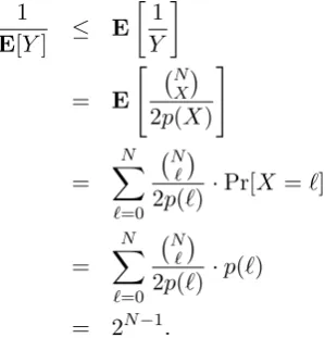
Theorem 7, we have that επ,$ is the expectation of 2p(X)/ NX
, i.e., επ,$ = E[2p(X)/ NX
6 COMPUTATIONAL RESULTS 16
LetY = 2p(X)/ NX
. Using Jensen’s inequality, we obtain
1
E[Y] ≤ E
1
Y
= E
" N
X
2p(X)
#
= N
X
`=0
N `
2p(`) ·Pr[X=`]
= N
X
`=0
N `
2p(`) ·p(`) = 2N−1.
Notingεπ,$ =E[Y] and ερ,$= 1/2N−1 gives the desired result.
6
Computational Results
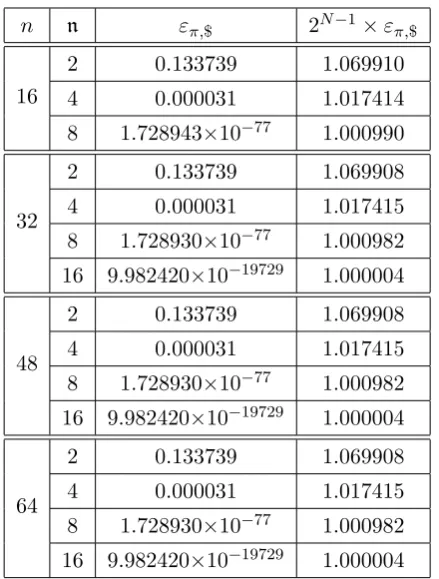
This section gives a summary of the computations done with the expressions of the error probabilities of non-linear invariant attack presented in Section 4 and 5. For computing επ,$ which is the error probability for distinguishing from a uniform random permutation, we have used the expression given by (29).
In our computations we have used the following Stirling’s approximation to compute the binomial coefficients.
k
i
≈ √ 1
2πk(i/k)i+21(1−i/k)k−i+ 1 2
.
The computations were done for n = 16,32,48 and 64; and N = 2n for n = 2,4,8 and 16, except that the case N = 216 was not considered when n= 16. Further, we have considered balanced g0 and gr, i.e., wt(g0) =
wt(gr) = 2n−1. As a result,ερ,$, which is the error probability of distinguishing from a uniform random function,
is equal to 1/2N−1.
Comparison between επ,$ and ερ,$. Table 1 gives the value of επ,$ and the ratio επ,$/ερ,$ = 2N−1επ,$ for
different values ofn and n. It may be noted that the last column of the table confirms Theorem 8 which shows that for balanced g0 and gr, επ,$ ≥ ερ,$ = 1/2N−1. Further, the ratio is close to 1. This may be explained by
referring to the proof of Theorem 8. The resultεπ,$ ≥1/2N−1is obtained using Jensen’s inequality to the convex
function f(x) = 1/x. It is known that Jensen’s inequality is tight when the convex function is a straight line. In the range of xwhere Jensen’s inequality is applied, it turns out that f(x) behaves almost like a straight line. Consequently, the inequality is almost tight in this range of applicability.
7
Conclusion
REFERENCES 17
n n επ,$ 2N−1×επ,$
16
2 0.133739 1.069910
4 0.000031 1.017414
8 1.728943×10−77 1.000990
32
2 0.133739 1.069908
4 0.000031 1.017415
8 1.728930×10−77 1.000982
16 9.982420×10−19729 1.000004
48
2 0.133739 1.069908
4 0.000031 1.017415
8 1.728930×10−77 1.000982
16 9.982420×10−19729 1.000004
64
2 0.133739 1.069908
4 0.000031 1.017415
8 1.728930×10−77 1.000982
16 9.982420×10−19729 1.000004
Table 1: Comparison betweenεπ,$ and ερ,$ = 2−(N−1).
Acknowledgement
An earlier version of this paper was entitled “Correlation Between (Nonlinear) Combiners of Input and Output of Random Functions and Permutations and Analysis of Nonlinear Invariant Attacks” and consisted only of the material in Section 2. A reviewer of the earlier version had suggested applying the techniques to the study of nonlinear invariant attack. We have been successful in doing so and are grateful to the reviewer for having provided this suggestion.
References
[1] Tomer Ashur, Tim Beyne, and Vincent Rijmen. Revisiting the wrong-key-randomization hypothesis. IACR Cryptology ePrint Archive, 2016:990, 2016.
[2] C´eline Blondeau and Kaisa Nyberg. Joint data and key distribution of simple, multiple, and multidimensional linear cryptanalysis test statistic and its impact to data complexity. Des. Codes Cryptography, 82(1-2):319– 349, 2017.
[3] Andrey Bogdanov and Elmar Tischhauser. On the Wrong Key Randomisation and Key Equivalence Hy-potheses in Matsui’s Algorithm 2. InFast Software Encryption, pages 19–38. Springer, 2014.
[4] Joan Daemen and Vincent Rijmen. Probability distributions of correlation and differentials in block ciphers. J. Mathematical Cryptology, 1(3):221–242, 2007.
A CHERNOFF BOUND 18
Advances in Cryptology - EUROCRYPT ’95, International Conference on the Theory and Application of Cryptographic Techniques, Saint-Malo, France, May 21-25, 1995, Proceeding, volume 921 ofLecture Notes in Computer Science, pages 24–38. Springer, 1995.
[6] Lars R. Knudsen and Matthew J. B. Robshaw. Non-linear approximations in linear cryptanalysis. In Ueli M. Maurer, editor, Advances in Cryptology - EUROCRYPT ’96, International Conference on the Theory and Application of Cryptographic Techniques, Saragossa, Spain, May 12-16, 1996, Proceeding, volume 1070 of Lecture Notes in Computer Science, pages 224–236. Springer, 1996.
[7] Mitsuru Matsui. Linear Cryptanalysis Method for DES Cipher. In Advances in Cryptology– EUROCRYPT’93, pages 386–397. Springer, 1993.
[8] Rajeev Motwani and Prabhakar Raghavan. Randomized Algorithms. Chapman & Hall/CRC, 2010.
[9] Luke O’Connor. Properties of linear approximation tables. In Bart Preneel, editor,Fast Software Encryption: Second International Workshop. Leuven, Belgium, 14-16 December 1994, Proceedings, volume 1008 ofLecture Notes in Computer Science, pages 131–136. Springer, 1994.
[10] Yosuke Todo, Gregor Leander, and Yu Sasaki. Nonlinear invariant attack: Practical attack on full SCREAM, iSCREAM and Midori64. Journal of Cryptology, 2018. https://doi.org/10.1007/s00145-018-9285-0.
A
Chernoff Bound
We briefly recall the Chernoff bound. This result can be found in standard texts [8].
Theorem 9. LetX1, X2, . . . , Xλbe a sequence of independent Poisson trials such that for1≤i≤λ,Pr [Xi = 1] =
pi. Then for X=
Pλ
i=1Xi and µ=E[X] =
Pλ
i=1pi the following bounds hold:
For any 0< δ≤1, Pr [X ≥(1 +δ)µ]≤e−µδ2/3. (31) For any 0< δ <1, Pr [X ≤(1−δ)µ]≤e−µδ2/2. (32)
B
Alternative Expression for
ε
π,$Lemma 4. Let P = (P1, . . . , PN) where P1, . . . , PN are chosen from {0,1}n under uniform random sampling without replacement. Let f :{0,1}n→ {0,1} be of weight w. Then
Pr[Ψ(f, P) = (0, . . . ,0)] = (
2n−w N ) (2n
N)
and Pr[Ψ(f, P) = (1, . . . ,1)] = ( w N) (2n
N)
. (33)
Proof. Consider the first statement. We need to consider f(P1) = 0, . . . , f(PN) = 0. This holds if and only if all of P1, . . . , PN fall outside the support of f. The probability that P1 falls outside the support of f is
(2n−w)/2n; given that P1 falls outside the support of f, the probability that P2 falls outside the support of f
is (2n−w−1)/(2n−1); given thatP1, P2 falls outside the support off, the probability thatP3 falls outside the
support off is (2n−w−2)/(2n−2) and so on. As a result we obtain
Pr[Ψ(f, P) = (0, . . . ,0)] = 2 n−w
2n ·
2n−w−1 2n−1 ·
2n−w−2 2n−2 · · ·
2n−w−N + 1 2n−N+ 1 = (2
n−w)(2n−w−1)· · ·(2n−w−N + 1)) 2n(2n−1)· · ·(2n−N + 1) ·
(2n−N)! (2n−N)!·
(2n−w−N)! (2n−w−N)!
=
2n−w N
2n N
B ALTERNATIVE EXPRESSION FOR επ,$ 19
The other statement is obtained similarly.
Lemma 5. Let F be a random (but, not necessarily uniform random) Boolean function. Let P = (P1, . . . , PN) where P1, . . . , PN are chosen from {0,1}n under uniform random sampling without replacement and these are independent of F. Then
Pr[Ψ(F, P) = (0, . . . ,0)] =
2n X
w=0 2n−w
N
2n N
·Pr[F ∈ Fw];
Pr[Ψ(F, P) = (1, . . . ,1)] =
2n X w=0 w N 2n N
·Pr[F ∈ Fw].
(34)
Proof. Consider the first statement.
Pr[Ψ(F, P) = (0, . . . ,0)]
= 2n X w=0 X f∈Fw
Pr[Ψ(F, P) = (0, . . . ,0)∧F =f]
= 2n X w=0 X f∈Fw
Pr[Ψ(f, P) = (0, . . . ,0)∧F =f]
=
2n
X
w=0 X
f∈Fw
Pr[Ψ(f, P) = (0, . . . ,0)] Pr[F =f] (sinceF andP are independent)
=
2n X
w=0 X
f∈Fw
2n−w N
2n N
·Pr[F =f] (from Lemma 4)
=
2n
X
w=0 2n−w
N 2n N X f∈Fw
Pr[F =f]
=
2n
X
w=0 2n−w
N
2n N
·Pr[F ∈ Fw].
The other statement is obtained similarly.
Theorem 10. Let g0 and gr be two n-variable Boolean functions. Let π be a uniform random permutation of {0,1}n andF =f
π[g0, gr] =g0⊕(gr◦π). Let P = (P1, . . . , PN) where P1, . . . , PN are chosen from {0,1}n under uniform random sampling without replacement and these are independent of F. Then
Pr[E0π] = Pr[Ψ(F, P) = (0, . . . ,0)] = m
X
x=0 2n−w
0−wr+2x N 2n N · w0 x
2n−w
0
wr−x
2n wr
;
Pr[E1π] = Pr[Ψ(F, P) = (1, . . . ,1)] = m
X
x=0
w0+wr−2x
N 2n N · w0 x
2n−w
0
wr−x
2n wr
.
(35)
Here w0 =wt(g0), wr =wt(gr) and m= min(w0, wr). Consequently,
επ,$ = Pr[Eπ] = m
X
x=0 2n−w
0−wr+2x N
+ w0+wr−2x
N 2n N · w0 x
2n−w
0
wr−x
2n wr
B ALTERNATIVE EXPRESSION FOR επ,$ 20
Proof. From Theorem 3, the possible values of the weight of F are w0 +wr−2x for x = 0, . . . ,m and for
w=w0+wr−2x, Pr[F ∈ Fw] = wx0
2n−w
0
wr−x
/ w2n
r
. Consider Pr[Eπ
0]. From Lemma 5,
Pr[Eπ
0] = Pr[Ψ(F, P) = (0, . . . ,0)] = 2n
X
w=0 2n−w
N
2n N
·
w0
x
2n−w0
wr−x
2n wr
= m
X
x=0 2n−w
0−wr+2x N
2n N
·
w0
x
2n−w0
wr−x
2n wr
.