1 The Daily and Hourly Rainfall Data Modeling using

(1)

Article

1

The Daily and Hourly Rainfall Data Modeling using

2

Vector Autoregressive (VAR) with Maximum

3

Likelihood Estimator (MLE) and Bayesian Method

4

(Case Study in Sampean Watershed of Bondowoso,

5

Indonesia)

6

Suci Astutik1_{, Umu Sa’adah}2_{, Supriatna Adhisuwignjo}3_{and Rauzan Sumara}4,_*

7

1_{Department of Statistics, Brawijaya University, East Java, Indonesia; [email protected]}

8

2_{Department of Statistics, Brawijaya University, East Java, Indonesia;}_{[email protected]}

9

3_{Department of Electronics Engineering, State Polytechnic of Malang, East Java, Indonesia;}

10

[email protected]

11

* Correspondence: [email protected]; Tel.: +6281909111417

12

13

Abstract: The hourly and daily rainfall data which is spatially distributed are required as an input

14

for run-off rain model. Furthermore, the run-off rain model is used to detect early flooding. The

15

daily and hourly rainfall data have characteristics that most of data are zero. Therefore we need a

16

model which can capture the phenomenon. A time series model involving location, which is a

17

model that can be developed to approach the daily and hourly rainfall data, we can call Vector

18

Autoregressive (VAR) model. The VAR model allows us for modeling rainfall data in several areas.

19

However, in certain conditions the VAR model often occurs over-parameterization and reduces

20

degrees of freedom. The aim of this study is to compare the VAR model with Maximum Likelihood

21

Estimator (MLE) and Bayesian to hourly and daily rainfall data in SampeanWatershed of

22

Bondowoso. The results showed that the hourly and daily rainfall data are fitted to VAR process of

23

orde 5 and 1 respectively. Based on the AIC and SBC values indicate that the Bayesian is better than

24

the MLE method. The Bayesian is able to predict parameters by producing a smaller variance

25

covariance matrix than the MLE.

26

Keywords: VAR; MLE; Bayesian

27

28

1. Introduction

29

Disasters in Indonesia increase from 2002 to 2015. According to the National Disaster

30

Management Agency the number of disasters which occurred in Indonesia is 143 disasters in 2002

31

and 1,681 disasters in 2015. Most of disasters in Indonesia are hydro-meteorological disasters such

32

floods. From 1 January to 8 February 2016, the National Disaster Management Agency recorded 103

33

floods in Indonesia and 74,369 people were affected by flooding. The areas affected by flooding are

34

East Java about 36 percent, Central Java 21 percent, Aceh 11 percent, West Sumatra 11 percent, Riau

35

7 percent, Jambi 4 percent, North Sumatra 4 percent, West Java 4 percent and West Nusa Tenggara 4

36

percent.

37

(2)

Therefore, it is necessary to have an early warning system about flooding in the areas. One of

38

solutions is by simulating and predicting rainfall in these locations. Simulations and predictions on

39

time series data such as rainfall data can use statistical models to explain dynamic of data. A

40

statistical model which allows us for modeling rainfall data in several areas at once is the Vector

41

Autoregressive (VAR) model.

42

Estimating parameter of the VAR model can use the Maximum Likelihood Estimator (MLE). In

43

many cases of using MLE, there are a number of problems such as over-parameterization and

44

collinearity. Therefore, Litterman [4], Sacakli [6] and Tahir [9] use the Bayesian VAR model to avoid

45

these problems. The aim of this study is to model hourly and daily rainfall data with the VAR model

46

using MLE and Bayesian and to compare the two estimation results based on the AIC and SBC

47

values.

48

49

2. Materials and Methods

50

2.1. Materials

51

We collected secondary data from Sampean Baru Waterhed, Bondowoso. The data are hourly

52

and daily rainfall in 7 rain stations these Sentral, Maesan, Ancar, Kejayan, Pakisan, Maskuning

53

Wetan and Sukokerto during January 2006 and January 2007, which is hourly data e.g

54

Sentral( , )and Maesan( ,), and daily data e.g Sentral( , ), Maesan( , ), Ancar( ,), Kejayan

55

( , ), Pakisan ( , ), Maskuning Wetan ( , ), dan Sukokerto ( , ). Stages of the analyses are (1)

56

Stationary test, (3) order VAR(p), (4) estimating parameter of VAR model using MLE and Bayesian,

57

(5) selecting the best model.

58

2.2. Methods

59

2.2.1. Order selection

60

Stationarity of data can be identified by looking at the Matrix Autocorrelation Function

61

(MACF) and Matrix Partial Autocorrelation Function (MPACF). Order selection would be difficult

62

if in the large matrix form, so Tiao and Box in Wei [11] noted the symbols (+), (-), and (.) in the (i, j)

63

position of the sample correlation matrix. The three symbols are explained in Table 1.

64

Table 1.The meanings of the symbols

65

Symbol Summary

+ Denotes a value greater than 2 times the estimated standard errors

- Denotes a value less than 2 times the estimated standard errors

. Denotes a value within 2 times the estimated standard errors

2.2.2. Matrix autocorrelation function (MACF)

66

According to Wei [11], a vector of time series is defined as , , … , then we can calculate

67

(3)

( ) = ( ) (1)

69

Where ( ) are the sample cross-correlations for the i th_{and j}th_{component series,}

70

( ) = ∑ ( , )( , )

∑ ( , ) ∑ ( , )

⁄ (2)

71

Where ̅ and ̅ are sample means of the corresponding component series.

72

2.2. 3. Matrix partial autocorrelation function (MPACF)

73

Tiao and Box in Wei [11] define the partial aautoregression matrix at lags, denoted by ( ), to

74

be the last matrix coefficient when then data are fitted to VAR process of orde s. Therefore, ( ) is

75

equal to , . The partial autoregression matrix function is defined as,

76

( ) =

′_{(1)[ (0)] ,} _{= 1}

′_{(s) −} ′_{( )[ ( )]} _{( )} _{(0) −} ′_{( )[ ( )]} _{( )} _{, > 1} (3)

77

covariance matrices (s) can be obtained by the sample covariance matrices (s),

78

(s) = ∑ ( − )( − )′_, _{= 1,2, …} ₍₄₎

79

where = ( ̅ , ̅ , … , ̅ ) is the sample mean vector.

80

2.2. 4. Vector Autoregressive (VAR) using MLE

81

Vector Autoregressive (VAR) model is one of multivariate time series models which has dinamic

82

interrelationship among variabels. Wei [11] defines stationary process of VAR(p),

83

′ ₌ ′_{+ ∑} ′ ′ ₊ ′ ₍₅₎

84

There are T observations, for = + 1, + 2, … , where p is VAR ordo. We have

85

= + (6)

86

where,

87

=

′

⋮

′

, =

′ _⋯ ′

⋮ ⋮ ⋯ ⋮

′ _⋱ ′

, =

′ ′

⋮

′

, dan =

′

⋮

′

88

where and are( − ) × matrices, is( − ) × (1 + ) matrix of observations, and

89

is(1 + ) × matrix of unknown parameters. Defined = − , likelihood function can be

90

writen,

91

( | , ) = (2 ) | | − ( − )′_{( −} ₎ ₍₇₎

(4)

and MLEs of and are

93

= ( ′ ₎ ′

94

and (8)

95

= ( )=( )′( )

96

2.2. 5. Vector Autoregressive (VAR) using Bayeisan or Bayesian Vector Autoregressive (BVAR)

97

Bayesian method is one of the estimation methods used to estimate parameter. There are two

98

important components in estimating using the Bayesian method, prior and posterior distribution.

99

Ntzoufraz [5] noted posterior distribution equal to likelihood function times prior distribution

100

which can be written,

101

( | ) ∝ ( | ) ( ) (9)

102

A conjugate prior is used in this case. According to Berger [1], prior and posterior distributions

103

in the conjugate prior have similar distributions. It is a multivariate normal distribution for

104

parameters and a wishart distribution for parameters. Kadiyala and Karlsson [2] stated that the

105

normal multivariate-wishart prior for BVAR models is better than normal multivariate-diffuse,

106

minnesota, and extended natural conjugate priorbased on RMSE (Root Mean Square Error) and

107

CPU-Time. Tahir [9] noted the normal multivariate-wishartprior is better than minnesota and

108

minnesota-wishart prior based on MSFE (Mean Square Forecast Error). Sims and Zha [7] added that

109

the normal multivariate-wishart prior is suitable in complex models. Koop and Korobilis [3] and

110

Sugita [8] define prior distribution of and ,

111

( ) ~ N( ( ), ) (10)

112

~ Wishart( , )

113

Where , , , are hyperparameter. Initialization of hyperparamter can use non

114

informative prior such as , , , and near to zero. The join posterior is obtained by the join

115

prior

116

( ) ∝ ( ( )) ( )

117

∝ | | −1

2 ( − )

′ ₍ ₋ _{) × | | | |} ₋1

2 [ ]

118

∝ | | | | | | − ( ) + ( − )′ ₍ ₋ ₎ ₍₁₁₎

119

with the likelihood function (7), so that the join posterior can be written,

120

( | ) ∝ ( | , ) ( )

(5)

∝ | | −1

2 ( − )′( − )

122

× | | | | | | −1

2 ( )

123

+ ( − )′ ₍ ₋ ₎

124

∝ | | | | | | − ( − )′_{( −} _{) +}

125

× − ( − )′ ₍ ₋ ₎ ₍₁₂₎

126

From the join posterior (12), we can derive the conditional posterior density for ,

127

( | , ( )) ∝ ( | )

( ( ))

128

∝ | | −1

2 ( − )

′_{( −} _{) +}

129

∝ | | − [ ] (13)

130

where = ( − )′_{( −} _{) +} _and ₌ _{− +} _{.So that the conditional posterior}

131

statistic form is

132

| , ( ) ~ Wishart( , ) (14)

133

Then we derive the conditional posterior density for ,

134

( ( )| , ) ∝ ( | )

( )

135

∝ −1

2 ( − )

′_{( −} _{) +} ₍ ₋ ₎′ ₍ ₋ ₎

136

∝ −1

2 ( − )′( ⊗ ) ( − )

137

+ ( − )′ ₍ ₋ ₎

138

∝ − ( − ∗)′ ( − ∗) (15)

(6)

where = + ( ⊗ ( ′ ₎₎ _and ₍

∗) = ( ) + ( ⊗ ) ( ′ ) ,

140

and we get the conditional posterior statistic form is

141

( ) | , ~ ( ( ∗), ) (16)

142

In this study we use Gibbs Sampler Markov Chain Monte Carlo (MCMC) methods to sample

143

the parameter of and . The conditional posterior distribution is used to process in Gibbs

144

Sampler algorithm.

145

2.2. 6. Markov Chain Monte Carlo (MCMC)

146

Markov Chain Monte Carlo (MCMC) methods are widely used in Bayesian inference.

147

According to Ntzoufraz [5], a Markov chain is a stochastic process { ( ), ( ), ( ), … , ( )_}_{such that}

148

( ( )_| ( )_{, … ,} ( )_{) = (} ( )_| ( )₎ ₍₁₇₎

149

In order to generate a sample from ( | ), we must contruct a Markov chain with two desired

150

properties. First, ( ( )_| ( )₎_{should be easy to generate from, and second, equilibrium}

151

distribution of the selected Marcov chain must be the posterior distribution of interest ( | ).

152

Assuming that we have met with these requirements, we then

153

1. Select an initial value ( ).

154

2. Generate R values until the equilibrium distribution is reached.

155

3. Monitor the convergence of MCMC. If convergence diagnostics fail, we then generate

156

more observations.

157

4. Cut off the first B observations (Burn-in Priod).

158

5. Consider{ ( ), ( ), … , ( )_}_{as the sample for the posterior analysis.}

159

We refers to analysis of the MCMC, ( ), ( )_, ( )_{, … ,} ( )_{. From this sample, for any function}

160

( ) of the parameters of interest we can

161

1.

Obtain a sample of the desired parameter ( ) by sample considering

162

( ( )_{), (} ( )_{), (} ( )_{), … (} ( )_{), … , (} ( )₎

163

2.

Obtain any posterior summary of ( ) from the sample using traditional sample estimates.

164

For instance, we can estimate the posterior mean by

165

( ( )| ) = 1

−

( )

166

and the posterior standard deviation by

167

( ( )| ) = 1

− − 1 (

( )_{) − ( ( )| )}

168

3.

Obtain other measures of interest might be posterior such as 2.5% and 97.5% credible

169

(7)

4.

Calculate Monte Carlo Error (MC Error).

171

2.2. 7. Gibbs Sampler

172

Gibbs Sampler is usually cited as a separate simulation technique because of its popularity and

173

convenience. One advantage of the Gibbs Sampler is that, in each step, random values must be

174

generated from unidimensional distributions for which a wide variety of computational tools exists.

175

Frequently, these conditional distributions have a known form and, thus, random number can be

176

easily simulated using standard function in statistical and computing software. Ntzouftaz [5] noted

177

the algorithm can be summarized by the following steps :

178

1. Set initial values,

179

( )_{= (} ( )

, ( ), … , ( ))

180

2. For = 1, … , repeat the following steps

181

( )

dari ( | ( ), ( ), … , ( ), )

182

( )

dari ( | ( ), ( ), … , ( ), )

183

( )

dari ( | ( ), ( ), ( ), … , ( ), )

184

. . .

185

( )

dari ( | ( ), ( ), … , ( ), )

186

3. Set ( )= and save it as the generated set of + 1 iteration of the algorithm.

187

2.2. 8. Information Criteria

188

Information criteria have been shown to be effective in selecting a statistical model. In the time

189

series literature, several criteria have been proposed. Two criteria functions are commonly used to

190

determine VAR model, these are AIC (Akaike Information Criterion) and SBC (Schwarzt Bayesian

191

Criterion). The best model is that produce the smallest AIC and SBC values. Tsay[10] provided to

192

calculate the AIC

193

= ln| | + (18)

194

and SBC

195

= ln| | + (19)

196

Here is observation, | | is determinant of variance-covariance matrix, is order model

197

and is variables.

198

199

3. Results

200

For check stationarity in data, we use Dickey-Fuller test (DF). The hypotesis of DF test is ∶

201

= 0 (data are non-stationary) vs ∶ < 0 (data are stationary), as shown on Table 1.

202

Table 2. Dickey-Fuller test

(8)

Data Variable df p-value Conclusions

low time-scale (hourly data) , -768.16 0.0001 Stationary

, -1128.20 0.0001 Stationary

high time-scale (daily data) , -15.40 0.0046 Stationary

, -20.53 0.0008 Stationary

, -13.14 0.0094 Stationary

, -18.15 0.0019 Stationary

, -30.70 0.0001 Stationary

, -20.12 0.0010 Stationary

, -15.86 0.0040 Stationary

Based on Table 2, probability values of statistic tests are less than (0.05), reject 0. So the data were

204

stationary. Order selection can be identified by looking at the Matrix Autocorrelation Function

205

(MACF) and Matrix Partial Autocorrelation Function (MPACF). If the time lag of MACF decreases

206

exponential or sinusoid whereas the MPACF is cut off at lag p, it is identified as the VAR(p) model.

207

these MACF and MPACF of hourly data based on Table 3 and 4.

208

Table3. Schematic MACF of hourly data

209

Schematic Representation of Cross Correlations

Variable/Lag 0 1 2 3 4 5 6 7 8 9 10

Sentral +. ++ ++ ++ ++ .+ .+ .+ .+ .+ ..

Maesan .+ .+ +. .+ .. .+ .+ +. +. .. ..

Table 4. Schematic MPACF of hourly data

210

Schematic Representation of Partial Cross Correlations

Variable/Lag 1 2 3 4 5 6 7 8 9 10

Sentral +. +. ++ .. .+ .. .. .. .. ..

Maesan .+ +. .. .. .+ .. .. .. .. ..

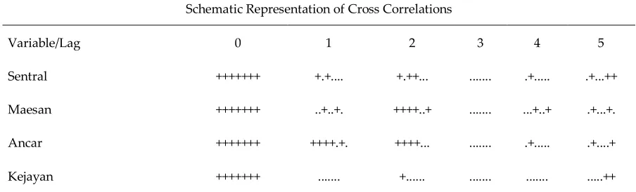
And Schematic MACF and MPACF of daily data based onTable 5 and 6,

211

Table 5. Schematic MACF of daily data

212

Variable/Lag 0 1 2 3 4 5

Sentral +++++++ +.+.... +.++... ... .+... .+...++

Maesan +++++++ ..+..+. ++++..+ ... ...+..+ .+...+.

Ancar +++++++ ++++.+. ++++... ... .+... .+....+

(9)

Variable/Lag 0 1 2 3 4 5

Pakisan +++++++ ... ... ... ... ...

Maskuning_Wetan +++++++ +.+.... +.++... ... ... .+...

Sukokerto +++++++ +++..+. +.++..+ ...+... ... ...

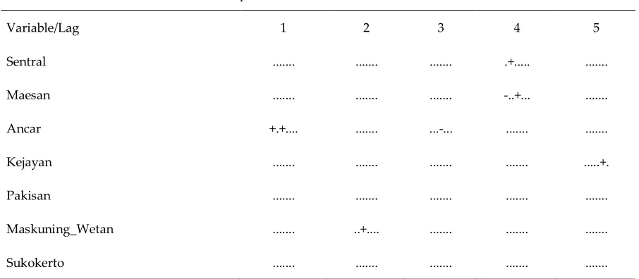
Table 6. Schematic MPACF of daily data

213

Schematic Representation of Partial Cross Correlations

Variable/Lag 1 2 3 4 5

Sentral ... ... ... .+... ...

Maesan ... ... ... -..+... ...

Ancar +.+.... ... ...-... ... ...

Kejayan ... ... ... ... ...+.

Pakisan ... ... ... ... ...

Maskuning_Wetan ... ..+.... ... ... ...

Sukokerto ... ... ... ... ...

From schematic MACF and MPACF above, we can conclude the hourly data following VAR(5)

214

process and the daily data following VAR(1) process. Estimating parameter is showed on Table 7

215

and 8.

216

Table 7.Estimation of VAR(5) parameter using MLE

217

Parameter Estimation Standard Error p-value

0.32857 0.02602 0.0001

0.03919 0.03044 0.1981

0.06520 0.02739 0.0174

0.10129 0.03060 0.0010

⋮ ⋮ ⋮ ⋮

0.01775 0.02309 0.4420

-0.00566 0.02567 0.8256

0.06263 0.02204 0.0046

0.16358 0.02523 0.0001

218

Table 8. Estimation of VAR(1) parameter using MLE

219

Parameter Estimation Standard Error p-value

-0.18800 0.16959 0.2591

-0.19337 0.23768 0.3496

(10)

-0.67658 0.42041 0.3327

⋮ ⋮ ⋮ ⋮

-0.09275 0.23840 0.6988

0.05637 0.20870 0.7881

-0.13940 0.42170 0.7423

0.23132 0.21750 0.2923

Based onTabel 7 and 8, VAR(5) model of hourly rainfall data is

220

, , = 0.32857 0.03919 0.02949 0.10497 , , + 0.0652 0.10129 0.00277 0.01727 , , + 0.08415 −0.03713 0,07183 0.05306 , ,

221

+ 0.01734 −0.01373

0.01775 −0.00566 , , + −0.0406 0.0399 0.06263 0.16358 , , + , , (20)

222

VAR(1) model of daily rainfall data is

223

⎝ ⎜ ⎜ ⎜ ⎜ ⎛ , , , , , , ,⎠ ⎟ ⎟ ⎟ ⎟ ⎞ = ⎝ ⎜ ⎜ ⎜ ⎛

−0.18800 −0.19337 0.85982 −0.67658 0.09860 −0.03643 0.63522

−0.05576 0.11628 0.22896 −0.07745 −0.09388 −0.11320 0.43326

−0.07923 −0.10828 0.88104 −0.75124 −0.06305 0.17090 0.67162

−0.08718 −0.00664 0.41018 −0.43418 0.13383 −0.21618 0.42185

0.03235 0.01375 0.19344 −0.22428 0.09159 −0.41097 0.44491

−0.06043 0.10110 0.13431 −0.12422 0.00324 −0.15626 0.31318

−0.13302 0.12277 0.26998 −0.09275 0.05637 −0.13940 0.23132⎠

⎟ ⎟ ⎟ ⎞ ⎝ ⎜ ⎜ ⎜ ⎜ ⎛ , , , , , , , ⎠ ⎟ ⎟ ⎟ ⎟ ⎞ + ⎝ ⎜ ⎜ ⎜ ⎛ , , , , , , , ⎠ ⎟ ⎟ ⎟ ⎞

224

(21)

225

The simulation process in estimating parameters with Bayesian method uses Gibbs Sampler

226

algorithm. Initial values in the simulation process are approximated by MLE. The first step of

227

simulation process generates the parameter then the second step generates the parameter . To

228

compile and run the MCMC algorithm for 10000 iterations and 500 burn in. It is divided into 97

229

batches for calculating MC error. The posterior summary is showed in Table 9 and 10

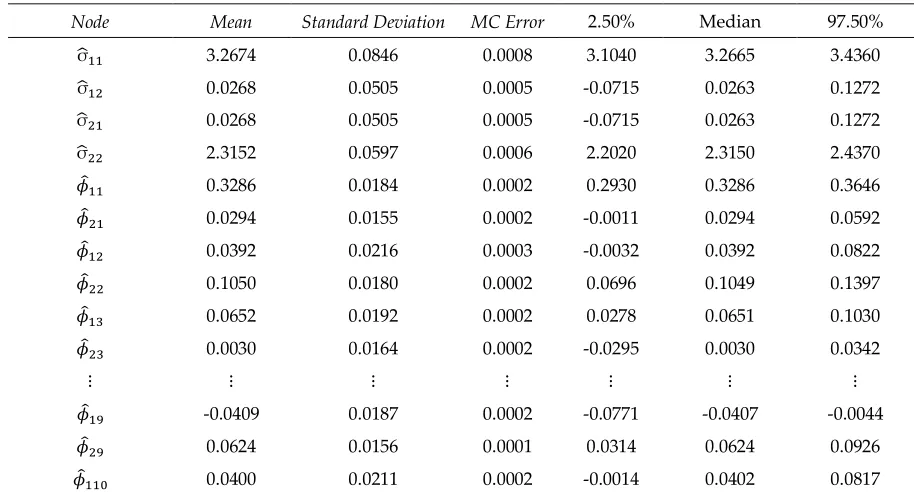
230

Table 9. Estimation of BVAR(5) parameter

231

Node Mean Standard Deviation MC Error 2.50% Median 97.50%

σ 3.2674 0.0846 0.0008 3.1040 3.2665 3.4360

σ 0.0268 0.0505 0.0005 -0.0715 0.0263 0.1272

σ 2.3152 0.0597 0.0006 2.2020 2.3150 2.4370

0.3286 0.0184 0.0002 0.2930 0.3286 0.3646

0.0294 0.0155 0.0002 -0.0011 0.0294 0.0592

0.0392 0.0216 0.0003 -0.0032 0.0392 0.0822

0.1050 0.0180 0.0002 0.0696 0.1049 0.1397

0.0652 0.0192 0.0002 0.0278 0.0651 0.1030

0.0030 0.0164 0.0002 -0.0295 0.0030 0.0342

⋮ ⋮ ⋮ ⋮ ⋮ ⋮ ⋮

-0.0409 0.0187 0.0002 -0.0771 -0.0407 -0.0044

0.0624 0.0156 0.0001 0.0314 0.0624 0.0926

(11)

0.1637 0.0179 0.0002 0.1286 0.1638 0.1990

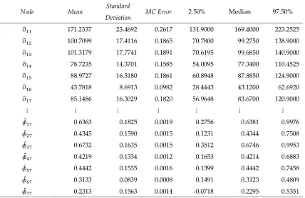
232

Table 10. Estimation of BVAR(1) parameter

233

Node Mean Standard

Deviation MC Error 2.50% Median 97.50%

σ 171.2337 23.4692 0.2617 131.9000 169.4000 223.2525

σ 100.7099 17.4116 0.1865 70.7800 99.2750 138.9000

σ 101.3179 17.7741 0.1891 70.6195 99.6850 140.9000

σ 78.7235 14.3701 0.1585 54.0095 77.3400 110.4525

σ 88.9727 16.3180 0.1861 60.8948 87.8850 124.9000

σ 43.7818 8.6913 0.0982 28.4443 43.1200 62.6920

σ 85.1486 16.3029 0.1820 56.9648 83.6700 120.9000

⋮ ⋮ ⋮ ⋮ ⋮ ⋮ ⋮

0.6363 0.1825 0.0019 0.2756 0.6381 0.9976

0.4345 0.1590 0.0015 0.1231 0.4344 0.7508

0.6732 0.1635 0.0015 0.3512 0.6746 0.9953

0.4219 0.1334 0.0012 0.1653 0.4214 0.6883

0.4442 0.1535 0.0016 0.1399 0.4442 0.7458

0.3133 0.0839 0.0008 0.1491 0.3123 0.4809

0.2313 0.1563 0.0014 -0.0718 0.2295 0.5351

Based on table 9 and 10, each of parameters is konvergence, because MC Error values are less than

234

1% standard deviation. If 2.5% and 97.5% percentiles does not contain a zero, the parameter will be

235

significant. We have BVAR(5) model of hourly data,

236

, , = 0.3286 0.0392 0.0294 0.1050 , , + 0.0652 0.1012 0.0030 0.0172 , , + 0.0845 −0.0374 0,0716 0.0530 , ,

237

+ 0.0174 −0.0136

0.0180 −0.0055 , , + −0.0409 0.0400 0.0624 0.1637 , , + , , (22)

238

and BVAR(1) model of daily data

239

⎝ ⎜ ⎜ ⎜ ⎜ ⎛ , , , , , , ,⎠ ⎟ ⎟ ⎟ ⎟ ⎞ = ⎝ ⎜ ⎜ ⎜ ⎛

−0.1866 −0.1923 0.8610 −0.6816 0.1009 −0.0404 0.6363

−0.0539 0.1167 0.2302 −0.0831 −0.0927 −0.1142 0.4345

−0.0802 −0.1078 0.8832 −0.7547 −0.0598 0.1671 0.6732

−0.0851 −0.0074 0.4104 −0.4376 0.1351 −0.2158 0.4219

0.0349 0.0137 0.1925 −0.2277 0.0933 −0.4120 0.4442

−0.0597 0.1012 0.1344 −0.1262 0.0041 −0.1558 0.3133

−0.1305 0.1229 0.2703 −0.0980 0.0584 −0.1401 0.2313⎠

⎟ ⎟ ⎟ ⎞ ⎝ ⎜ ⎜ ⎜ ⎜ ⎛ , , , , , , , ⎠ ⎟ ⎟ ⎟ ⎟ ⎞ + ⎝ ⎜ ⎜ ⎜ ⎛ , , , , , , ,⎠ ⎟ ⎟ ⎟ ⎞ (23)

240

The model selection uses AIC and SBC values. The AIC and SBC values are showed in Table 11

241

bellow,

242

Table 11. AIC and SBC values

243

Model Estimation Method AIC SBC

VAR(5) MLE 3.4257 3.4972

(12)

VAR(1) MLE 33.5855 35.2811

Bayesian 29.7573 31.4385

It shows that Bayesian method is better than MLE, because the AIC and SBC values are smaller than

244

MLE method.

245

4. Discussion

246 Based on Table 2 - Table 6 it can be seen that hourly and daily rainfall data have fulfilled the

247 stationary assumption, which is the assumption of the VAR model. The corresponding hourly

248 and daily rainfall models are VAR (5) and VAR (1), respectively, seen from MACF and

249 MPACF. The estimation results of the VAR(1) model parameter for daily rainfall data with

250 the MLE method (Equation 20) and the Bayesian method (Equation 22) produce values that

251 are not much different. So do the VAR(5) model for hourly rainfall data by the MLE

252 method (equation 21) and the bayesian method (Equation 23). This shows that the MLE and

253 bayesian methods provide the results of estimating the parameters of the VAR model that are

254 almost the same. However, based on the AIC and SBC values (Table 11) shows that the

255 Bayesian method produces a VAR model with smaller AIC and SBC values compared to the

256 MLE method for both hourly and daily rainfall data. This means that in hourly and daily

257 rainfall data, the Bayesian method produces a VAR model that is better than the MLE

258 method.

259

5. Conclusions

260

We can conclude that the hourly rainfall data and daily rainfall data at Sampean Bondowoso

261

watershed station follow VAR(5) and VAR(2) respectively. The criteria of best models show that

262

parameter estimation using Bayesian method is better than MLE method, because Bayesian method

263

is able to predict parameters with the smaller variance matrix than MLE method.

264

Acknowledgments: Thank you to Kemenristekdikti for the support of research funding in the Fundamental

265

Research Grant 2018, the Rector of Brawijaya University, the Dean of FMIPA and the Chair of the Mathematics

266

Department of Brawijaya University for the support of the permission and funding assistance for this

267

conference.

268

269

References

270

271

1. Berger, J.O. Statistical Decision Theory and Bayesian Analysis, Second Edition, Springer, New York, 1985.

272

2. Kadiyala, K.R.; Karlsson, S. Numerical Methods for Estimation and Inference in Bayesian VAR-Models, Journal

273

of Applied Econometrics.12 (1997), pp. 99-132.

274

3. Koop, G.; Korobilis, D. Bayesian Multivariate Time Series Methods for Empirical Macroeconomics, University of

275

Strathclyde, Galasgow Scotland, 2010.

276

4. Litterman, R.B. Forecasting with Bayesian Vector Autoregressive : Five Years of Experience, Journal of Business &

277

Economic Statistics. 4 (1986), pp. 25-38.

278

5. Ntzoufras, I. Bayesian Modeling Using WinBUGS, John Wiley & Sons, United States, 2009.

279

6. Sacakli, I.S. Do BVAR Models Forecast Turkish GDP Better Than UVAR Models ?, British Journal of

280

(13)

7. Sims, C.A.; Zha, T. Bayesian Methods for Dynamic Multivariate Models. International Economic Review.

282

39(1998), pp. 949-968.

283

8. Sugita, K. Bayesian Analysis of a Vector Autoregressive Model With Multiple Structural Breaks,

284

Economics Bulletin. 3(2008), pp. 1-7.

285

9. Tahir, M.A. Analyzing and Forecasting Output Gap and Inflation Using Bayesian Vector Auto Regression (BVAR)

286

Method: A Case of Pakistan,International Jurnal of Economics and Finance.6 (2014), pp. 233-243.

287

10. Tsay, R.S. Multivariate Time Series AnalysisWith R and Financial Applications, John Wiley & Sons, Canada,

288

2014.