Connection Indexing of 2D Binary Images on Hexagonal Grid for Digital Image Representation and Retrieval

VICTORIA ~ UNIVERSITY

+l

DEPARTMENT OF COMPUTER AND

MATHEMATICAL SCIENCES

Connection Indexing of 2D Binary Images

on Hexagonal Grid for Digital Image

Representation and Retrieval

Z. J

. Zheng and C

.

H. C

. Leung

(52 COMP 19)

February, 1995

(AMS

: 58010, 57M99)

TECHNICAL REPORT

VICTORIA UNIVERSITY OF TECHNOLOGY

(P 0 BOX 14428) MELBOURNE MAIL CENTRE

MELBOURNE, VICTORIA,

3000

AUSTRALIA

Connection Indexing of 2D Binary Images on Hexagonal Grid

for Digital Image Representation and Retrieval

Z.J. Zheng and C.H. C. Leung

Department of Computer and Mathematical Sciences, Victoria University of Technology

ABSTRACT

In exploring digital libraries on a network environment, it is important to have efficient indexing schemes to represent and retrieve digital images. To meet practical requirements, a new connection indexing for binary images on hexagonal grid is proposed. Not only could the new indexing generate Euler number, but it can also be use to explore complex boundary effects for bounded and unbounded binary images of hexagonal grid in general. The connection indexing provides a global invariant between a number of objects incident with image boundaries and the number of uncertain areas isolated in objects within a binary image. This indexing "provides invaluable information to describe intrinsic boundary effects. Using connection indexing, it is possible to provide a set of local, intermediate and global invavriants in terms of discrete topology and connectivity for rapid representation and retrieval of images by contents. Sample pictures and their indexing are also presented.

Keywords: Discrete Geometry, Convexity Analysis, Global Topology and Connection Invariants, Pattern Recognition, Digital Library, Image Retrieval, Automatic Indexing

1. Introduction

1.1. Image Representation and Retrieval in Digital Libraries

With present day internet facilities, it is now convenient to retrieve multimedia information from digital libraries through. networks. However, it is much more time-consuming to retrieve images than text over a network, and even for a small-sized image, it is necessary to have a fetching time longer than that required for several text pages. Because modem multimedia databases contain many images, in addition to requirements for compressions and high speed commnications, it is important to have efficient schemes to represent and retrieve images by contents. To explore future digital libraries on networks, it is necessary to investigate possible schemes of automatic indexing of images. Some kinds of images (such satellite images,cell pictures, micro-organization, CT images and so on) may be properly described by their intrinsic geometric and topological configurations. To meet practical requirements, it is helpful to use different indexing techniques representing intrinsic features of images to increase the efficiency of digital libraries for automatically representing and retrieving images.

1.2. Euler Number and Limitations

investigate their local and global invariant properties. The Euler number is one of the best known invarinats in topology. Its discrete form for binary images plays a key role in digital image representations [Kong and Rosenfeld 89]. The Euler number is defined as the difference between the number of objects and the number of holes denoted by E. The capital letter 'B,' for example, has a Euler number of -1 (E('B')

=

-1) since it is an object with two holes. The letter 'i' has a Euler number of 2, the letter 'I' has a Euler number of 1 and so on.

Many researchers have given formulae for computing Euler numbers for binary images. As is well-known that connectivity of binary image points on hexagonal grid does not have connectivity paradox [Rosenfeld 70], it is assumed that both foreground and background have the consistent Euler numbers. Using the critical point approach, Gray [Gray 71 ], for example, gave a simple equation to calculate the Euler number for binary images on hexagonal grid by counting the number of the two blocks X 8 =

0 0

and V₈ = 0 in six directions over the image respectively.

1 1 1

Defining

I;

as the number of X₈ in the image having one 1 and two O's, in any of the six orientations and similarly defining

I;

for V₈, then adding the six directions will give its the Euler

number E = (

T., -

I;)

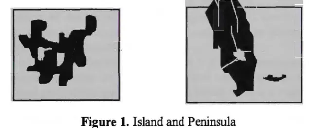
I 6.

There are several limitations behind this kind of approach. For example, ·considering the letter 'i', the Euler number of 2 can be calculated only if two objects can be isolated in a given region and boundary effects of the region can be ignored. When the letter 'i' is bounded in a bounded region, its background could be explained as two holes in one object. The Euler number for this is -1, the same as the letter 'B'. In more complex situations such as processing satellite images of Florida peninsula, it is not feasible to directly use the above scheme to calculate Euler number because boundary effects cannot be ignored. Two pictures for such situations are illustrated in Figure 1.

Figure 1. Island and Peninsula

Since the previous ,expression for Euler number is only based on the number of detailed patterns for 1 points in an isolated unbounded region, it cannot be .used in general for representing an image which has many parts of objects connected with their other parts outside the image. In other words, investigators have established the representations between the numbers of local patterns for 1 points and one of the global topological invariants, but the relationships among their subimages and complex boundary effects were ignored or over-simplified. To describe an image with complicated connections to neighbouring areas, more investigations need to be carried out.

[Zheng and Maeder 91, 92a] a new convexity index for 1 points is proposed to analyze a pyramid hierarchy for connectivity analysis of binary images. In addition, a balanced scheme of convexity index for both 1 and 0 points has been proposed and systematically developed in [Zheng 94a] for the conjugate classification of binary images on rectangular grids.

2. A New Scheme for Representing Boundary Effects

In this paper, connection indexing using convexity index is proposed for a bounded or unbounded binary image on hexagonal grid. Using patterns of the kernel form of hexagonal grid, it is feasible to assign each point in a binary image of hexagonal grid in one of eight values in relation to convexity index. Summing up all convexity indices over an image, connection indexing is generated. The differences exist between bounded and unbounded images, how connection indexing can be used to describe binary images with intrinsic boundary effects and what is the intrinsic relationship between traditional Euler number and connection indexing are studied.

The organization of the paper is as follow. The kernel form, bounded and unbounded patterns, convexity index for hexagonal grid are defined in section 3. Connection Indexing, singular and non-singular points, bounded and isolated images are described in section 4, and the essential properties of connection indexing are investigated. The main result of this paper is givend in Proposition 4.4.4. Sample images and their connection indexing are illustrated in section 5.

3 Kernel Form and Convexity Index

3 .1. Kernel Form of Hexagonal Grid

The hierarchical classification of the kernel form of hexagonal grid is established in [Zheng and Maeder 92] and further systematical investigations are undertaken in [Zheng 94a]. The main structure of the kernel form may be summarized as follows.

Let X denote a binary image on the hexagonal grid, x E X be a given point of the image. The

simplest scheme for connection indexing on the hexagonal grid uses seven adjacent grid points (the

kernel form of the hexagonal grid) as the pattern form. The kernel form is a regular form composed

of seven grid points for which one point x is at the center and another six neighbouring points

x₀ - x

5 are around it. The kernel form can be denoted by K(x). When each point is allowed to assume values of only I or O; seven points have fixed values as a pattern (unbounded pattern) denoted by S ( x), and there is a total of 2 7 = 128 patterns as a pattern set denoted as

n

for the kernel form; when at least one of six neighbouring points is allowed to assume an uncertain value denoted by '*', and seven points are composed of a bounded pattern denoted by S'" ( x), and there is a total of 2 x 36

K(x)=x

₅ x _{x2 ;}

x e{0,1}, xi e{O,L *};

xo

S(x)=x

₅ x

x,xi e{O,l}; s*(x)=x

₅ x

xi;

x,xi e{O, 1}

&

3xi e{*};

Figure 2. Kernel Form and Patterns

By convention, It is assumed that each bounded pattern can be simplified into a pattern to replace each

*

point by the value

-.x

mapping the pattern

s• (

x) surjectively into an unbounded pattern S ( x). A pattern S ( x) has a unique conjugate pattern, denoted as

S (

x), with S ( x)

=

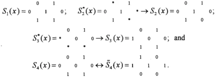
-,S ( x), representing each point in the conjugate · pattern has the opposite value corresponding to the original point.

Some examples of bounded and unbounded and conjugate patterns are as follows:

0 _* 0

S₁ (x) = o o·

' s;(x)=o • ~S2(x)= o o· '

* 0

0 0

s;(x) = * 0 0 ~

s3

(x) = 1 0 o·

' and

* +.

0 0

S_{4 (x)} = o 0 o~S4(x)=1 1 . 0 0

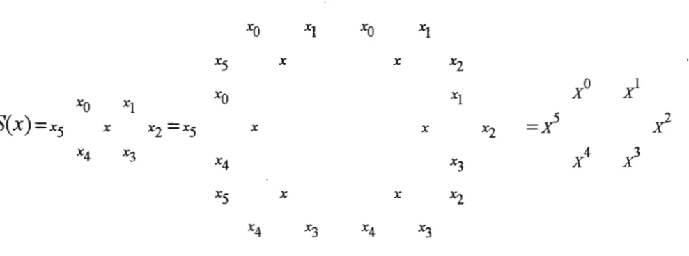
3 .2. Convexity Function and Convexity Index

XO XI xo XI

x5 x x x2

xo xo XI

XO xl

xl

S(x)=x5 x x2 =x5 x x _xi =X5

x2

X4 X3

X4 X3 x4

x3

X5 x x X2

X4 _~ X4 _~

Figure 3. Six Overlapped Blocks of Pattern

Since the point x occupies the most important position, central position, in a pattern S ( x), a

. X. I Xi convexity function needs to be defined relative to x. By convention, let Xi = 1

-x Xi+I j-l, j+l (mod6) o-.:;j-.:;5.

Definition 3.2.1. For any pattern S ( x) and its six blocks {Xi} ~=o, the j -th convexity function

J

i

lS

1, Xi

E{o

0 _0' I

i};

0

J/S(x)) = -1, Xi

E{1

0 0 1 0 }; O< . <5

I ' 0 - } - .

0, otherwise;

Proposition 3.2.2. For a point x, if its convexity function

Ji (

S ( x)) has a value of 1 (-1 ), then its

j-th neignouring pointy (xi) has a value of -1 (1) for the convexity function fk(S(y )), where

k = j

+

3 (mod 6).

Proof. Let S ( x) and S (y) be two neighbouring patterns,

X I

Xi =

1-x _Xi+I and

yk

=

Yk+I Y , where Yk

=

x andy = xi. The result follows as noting that the k-th

Yk Yk-I

Corollary 3.2.3. For a point x, if f; ( S ( x))

=

I (or - I), then there is a ; (or - ; ) exterior angle

around x.

Proof. This property is evident on viewing each point as a small hexagonal block. •

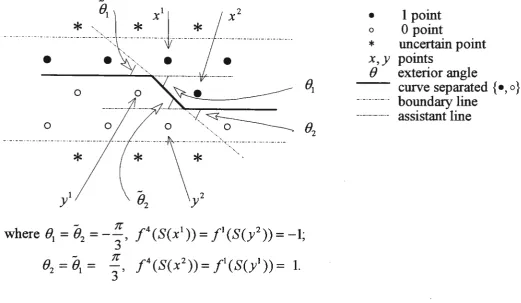
An example illustrating Proposition 3.2.2 and Corollary 3.2.3 is shown in Figure 4.

0

*

*

•

0

*

x,y

e

Figure 4. Exterior Angles and Convex Functions

1 point 0 point

uncertain point points

exterior angle

curve separated { •,

o}

boundary line assistant line

Using the family of convexity functions, a more useful number, a convexity index, can be defined.

Definition 3.2.4. For any pattern S ( x), the convexity index denoted by v 1s

5

v(S(x)) = Lf/S(x)).

0 ₀

For example,

S

₁(x) = o

0

0 ₀

S3(x)= 1 0 0' v(S3 (x)) = -1; S4(x)=o 0 o, v(S4(x)) = -1;

0

S4(X)=1 _{l ' v(S4(x)) =} -1; S5(x)= 1 0 1, v(S5(x))=6. 0 0

3 .3. Essential Property of Convexity Index

Proposition 3.3.1. For any pattern S(x ), v(S(x )) = v(S(x)).

Proposition 3.3.2. For two patterns S(x), S(y), if S(x) can be transformed by cyclic

permutations of its six neighbouring points to S (y), then v( S ( x)) = v( S (y)) .

Proof. The cyclic permutations of neighbouring points only change subscripts of the points. •

Lemma 3.3.3. There are 28 classes of rotational invariant patterns for the pattern set of the kernel

form of the hexagonal grid [Zheng and Maeder 92b].

Proposition 3.3.4. For a pattern S(x), the value of v(S(x)) is in the· set {6, 3, 2, 1, 0, -1, -2, -3}.

Proof. Since

-1sfjs1

=>

-6

s

_L!j

s

6, the value of v(S(x)) is in {-6, ... ,6}. Only ifthe central

point is different from six neighbouring points, v = 6. If there is one neighbouring point with the same v~ue as x, then only three convexity functions can have a value of 1. So it is impossible for the index to have a value in { 4, 5}. Because each function with a value of -1 need to satisfy x = _{xj_1} = xj+l-::/:- xj, it is impossible for v(S(x)) to have a value in {-4, -5, -6} .

•

Corollary 3.3.5. Using the values of (x, v), V S(x) E 0, S(x) can be partitioned into 16 classes.

3.4. Singular and Non-Singular Points

Definition 3.4.1. For a point x in a binary image, it is a non-singular point if v( S ( x))

=

0,

otherwise, it is a singular point.

Proposition 3.4.2. Only points in 38 patterns of eight rotational invariant classes are non-singular,

other points in 90 remaining patterns of 20 classes are singular.

Proof. For x = O points, there are 19 patterns in four classes. One pattern ts m

~

1

( x)

= {

0 : o :

+

each class of

~

2

( x)

= {

o : o :

+

~

3

<i>'(x)

= { 1 :

o : o}

contains six patterns in different orientations. Reversing all points

from e1-o, 0-1) for each pattern, another 19 patterns in the four conjugate classes,

<1>1 ex), <1>2 ex), <1>3 ex) and <1>4 ex), can be determined. •

The eight non-singular classes play an important role in the investigations in section 4.

3.5. Boundary Points and Bounded Images

For a digital image X in a given domain, grid points of image belong to four parts: interiors e0)

and boundaries e b') for Inside e+ ) and Outside

C )

of X denoted as 0+ e X), 0-e X), b' + e X) and

o-(X) respectively. That is, 0+ ex),

a+

ex) c X and 0-ex), a-ex) CZ: X .

An image Xis a bounded image, if there is at least one point in

a -

e

X) and the point is an uncertain point *. An image

x

is a full bounded image, if Vx Ea -

e

X) => x E {*}' that lS,

Vy E b' +

e

X) =>

sey)

E

!l"'.

Moreover, the image X is an unbounded image, if

Vx Ea +ex)=> sex) E.0.

In general, an unbounded image needs to satisfy much stronger conditions than a bounded image, all points in 0+ex), a+ex), and a-ex) have to be in fixed values. However, for merely two parts: 0+ex), and b'+(X) need to be determined at least for a bounded image.

A binary image Xis an isolated image if there are points in X with two values and all points in

a+ex) have only one value. By convention, all 0 points inX can be collected, denoted as D₀ex),

and similarly remaining 1 points in X denoted as D₁

e

X).

4. Connection Indexing and Properties

4. 1. Connection Indexing

Definition 4.1.1. For a subimage W in a bounded image X, W c X, connection indexing denoted

1

as cew) is C(W) = -

L

vesex)). 6 xEW

The definition of connection indexing is flexible and general. Since a subimage W can be selected as random point set from X, the sum of convexity index for the image could be a rational value. If the indexing is useful, detailed investigations are required. For representing arbitrary images, it is essential to apply connection indexing to an image in a simply connected domain first.

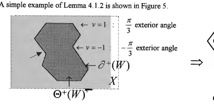
Lemma 4.1.2. For a binary image X, if a subimage Wis simply connected and outside boundaries

Proof. Since x E 0 + (W)

=>

S ( x) E <1>1 or <i>1 and v( S ( x)) = 0, outside boundaries of all points in

a+

(W) are composed of a simply closed curve and

L

v(S(x)) = 6. Using Corollary 3.2.3, 'VxE o+(X)

this is equivalent to sum up all exterior angles around the closed curve. •

A simple example of Lemma 4 .1.2 is shown in Figure 5.

. ---· -·-·-· -·--~ ----·-·---·-· -·-·--_, -. ---·-. -· ---·-. ---,

; ; 1C

! - exterior angle

\ 3 '

i 1C •

! - - exterior angle

i 3

'

o+(r)

Xi

. _. __ --~---. --·-· -~-. --·-·-. -·-· -·-·-· -·-·-·-r-- ·-· -. ---. ~

e+(W)

Figure 5. An Image and Close Curve

4.2 Connection Indexing for Unbounded and Isolated Images

=>

i

Closed Curve

Proposition 4.2.1. For an image X and its unbounded subimage W c X, if Wis isolated and \ix Ea+ (W), S(x) E <1>1 or <i>1

then C(W) = 0.

Proof. Since all points in 8

+

(W) are inner points in the same value, only points in

e+

(W) may have non-zero convexity functions. Since all convexity function values are paired in 0 + ( W) regions. This makes connection indexing vanish. •

Corollary 4.2.2. For a subimage W c X under the same condition as Proposition 4.2.1.,

cl

(W)

=

L

v(S(x)) = -Co(W)

=

L

v(S(x)).

xED₀(W)

Proof. C(W) = C₁ (W)

+

C₀ (W) = O

=>

C₁ (W) = -C₀ (W). •

Corollary 4.2.3. For a subimage W c X under the same condition as Proposition 4.2.1, ifthere are

n objects and m holes for I points, then there are m object with n holes for 0 points. Each object provides a value of 1 and each hole provides a value of -1 to connection indexing.

In convention, a closed curve around an object (a hole) is called a convex cycle (a concave cycle).

Corollary 4.2.4. For a sub image W c X under the same condition as Proposition 4 .2. 1, if 8 + (W) is composed of 0-points, then C₁ (W) = E(W).

From Corollary 4.2.4, there is an accurate correspondence between the Euler number and

connection indexing. Both 0 and 1 points share a uniform equation of connection indexing.

Differences come from selected points of the image. As mentioned before, in calculating the Euler

number, it is essential to ignore all boundary effects. To use connection indexing, it is necessary to

investigate bounded conditions.

4.3. Connection Indexing for Bounded and Isolated, and Unbounded Images

Proposition 4.3.1. For a full bounded and isolated image X, there is at least one singular point.

Proof. Under full bounded and isolated conditions, any x, y E a + ( X) => x = y and patterns

S(x),S(y) Eil*. If there is no a singular point in a+(X), then '\Ix EO+(X)

=> S ( x) E { <1>3, <1> 4

} or { ci)

3

, ci)4}, they are composed of a closed circle around

e

+

(

X). If

o

+ ( X) is removed from X, and the points in 8 + (

E>+ (

X)) still do not have a singular one,

then the similar procedure of the removal can be repeated. After a finite number of removals,

the remaining part has to be either an isolated point or a single line or a block in two point

width and so on. Any remaining object has at least one singular point. •

Proposition 4.3.2. For a full bounded and isolated image X, there is C ( X) = I.

Proof. For all points in

e+

(X), all convex and concave cycles are paired, and only one convex

cycle composed by

o

+ ( X) remains. •

It is well-known that a simply connected object makes a pair of convex and concave cycles.

However, if there is only partial object in the selected region, then significant boundary effects cannot be simply ignored.

Proposition 4.3.3. For an unbounded image W, if for '\Ix Eo+(W) and '\/j,f/S(x))

=

0, then

C(W)= 0.

Proof. If::Jx EW and fj(S(x))-:t= 0, then x E0+(W). From Proposition 3.2.2, connection indexing

of W vanishes.•

Proposition 4.3.4. For an unbounded image W, if C(W)-:t= 0, then :ix Ea+ (W), f/S(x))-:t= 0.

Proof. By f/S(x))'s pair and local properties and Proposition 4.3.3, only if :Jx Eo+(W) and

:Jy Eo-(W), fj(S(x)) and fk(S(y)) are a pair of opposites, then the value of f/S(x))

contributes to C(W). •

Since pairs of local opposite properties come from convexity function, it is difficult to

investigate detailed configurations of 8 + (W) in general. Conditions in Propositions 4. 3. 3 and 4. 3. 4

will be satisfied in unbounded images in general. Under the unbounded condition, connection

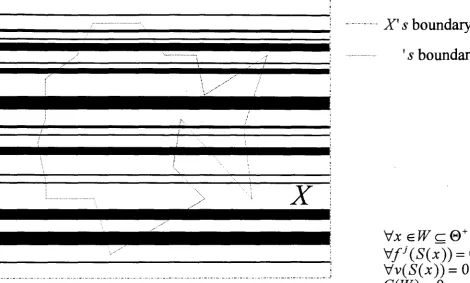
indexing is either O or a rational number. For some images composed of non-singul.ar points, s~ch

as streak line images, even a subimage selecting all points from unbounded and arbitrary domams,

-- -·-·-·-·-·-·- -·-- - - · -·- - - -·-·- · - -·-· -· --·- -1

'

·~·--···-~

f'·.

·· ..

~>

x

'

-· -. -. -· - ·-· -• - ----·-. -· -• -· -·-. -• ---. -. - ·-. - --. -. -. ---·-. ---·-· -• -. -· -·-. -. -·-· -·-. -· ---. -·-· -·-· - . -·-· -·-. .J

-

---

---

-

X'

s boundary line

's

boundary line

'\Ix

EW

c

e+(X),

Vf

1

(S(x))

=

0,

Vv(S(x))

=

0 and

C(W)

=

0.

Figure 6. Streak Line Image X and Unbounded Subimage W

4.4. Connection Indexing for Bounded Images

In Proposition 4.3 .2, it is shown that even an isolated bounded image, connection indexing has a different value from an unbounded condition.

Definition 4.4.1. For a bounded image X, there are two unbounded canonical images denoted as

X" and .

.X-*.

For any entry

[i,J]

point on the grid,

and

*[

.

·]

{X[i

,

J],

if

[i, J]-

th point in the bounded area of

X;

x

l J =

' 0, otherwise;

-

*[.

·

]

{X[i,

J],

if the

[i,

J]-

th point in the bounded area of

X;

x

l J =

' 1, otherwise.

x

x"'

x

-.

In

D

or r:·:·:·:·:·_-_-:-]I 0 points; _{: 1 points;}

l

l

!.,J=J~::

_,

J·:l·.

·

=:l:~J[:

_{I :}

*

_{uncertain points.}

Figure 7. A Bounded Binary ImageX and Two Unbounded Canonical Images X"' and

.k*

Proposition 4.4.2. For a bounded imageX, C(X) = C₀(X"')

+

C₁ (X"').

Proof. C0 indexing is the sum for all 0 points of

X"'

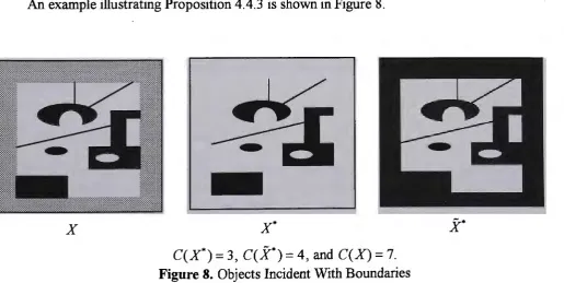
and C1 for all 1 points of X"'. •

Proposition 4.4.3. For a simply bounded image X, C(X)

=

n,

where

n

is the number of objects incident with t3 + ( X) .

Proof. From Proposition 4.3.2, for any object in e+(X), the pair effects of convex and concave cycles are balanced out. Only objects incident with iJ+(X) are affected. Since objects for both 1 and 0 points, each one provides a convex cycle, so there is such a value of C( X). •

An example illustrating Proposition 4.4.3 is shown in Figure 8.

x

x"'

x

-.

C(X"') = 3, C(X"') = 4, and C(X) = 7.

Proposition 4.4.4. For a bounded image X, C(X) =

n- m,

where

n

is the number of objects incident with boundary and mis the number of uncertain areas isolated in objects.

Proof. If an uncertain area isolated in an object, then there is a hole in either

x·

or

x•

.

This

?ro_vi~es a concave cycle. However, if this uncertain area is not isolated in an object, its effect 1s surular to other uncertain areas to make each object incident with the area a convex cycle. •

An example of Proposition 4.4.3 is illustrated in Figure 9, where there are 2 uncertain areas in X

and 10 objects (n = 10) incident with boundaries, and only one uncertain area (m= I) is isolated in an object. So there are C(X*)

=

4, C(X*)

=

5, and C(X)

=

4

+

s

= 10-1=9.

x

x

-.

Figure 9. Objects and Isolated Uncertain Area (n=IO, m=l)

Proposition 4.4.4 is the main result of this paper. An accurate equation is formulated for a bounded image in relation to the number of objects incident with its boundaries and the number of uncertain areas isolated in objects. Not only could connection indexing generat,e invariants with comparable meaning as the eminent Euler number under unbounded and isolated conditions, but also the global invarinat provides a new meaning in relation to the number of objects incident with boundaries. It is interesting that the number C( X) itself can automatically ignore the complicated object configurations isolated in the given domain, and it represents intrinsic connection invariants relevant to boundary effects.

5. Use of Connection Indexing

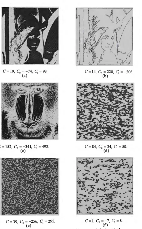
In order to illustrate the usefulness of connection indexing, sample images on hexagonal grid are selected. Six pictures (a)-(f) and connection indexing are listed shown in Figure 10. Picture (a) is a binary image ofLenna in 512x512. Three indices C₀,C₁ and Care listed under the picture. Picture (b) is an edge image of picture (a). Some interesting differences exist. Picture (a) has more objects than holes for 1 points, and picture (b) has more holes composed by 1 points, however the index C

C

=

19,

C

0

= -

74,

C

1

=

93.

(a)

C

=

152, C0

=

-341, C1

=

493. (c)

C

=

14, C0

=

220, C1

=

-206.

(b)

C

=

39, C₀

=

-256, C1

=

295. C

=

1, C0

=

-7, C1

=

8.

(e) (f)

'

noticed that both C0 and C1 are two pos1t1ve integers. Compared with other images, objects for both points have stronger connection to its boundaries. Picture ( e) is a O line dominant image, it has a reasonable number of objects incident with boundary and finally picture (f) is an image with an interior part similar to a cell image. However, connection indexing C=l indicates that it is an isolated image. You can check boundaries of the image carefully, its interior boundary is composed of points in the same value. From C0 and C1, it is obvious that there are more objects than holes for

1 points in the image. Differences among these pictures and their connection indexing are significant. From these examples, more valuable information can be extracted by the use of three global invariants for representing the intrinsic features of an image. All shown pictures and connection indexing are generated from an implemented prototype of the conjugate transformation of the hexagonal grid with some extension functions for automatically indexing for image databases.

The current system is implemented on Silicon Graphics Indy computer.

6. Conclusion

A new connection indexing for binary images on hexagonal grid has been presented. Its theoretical foundation is established, and its essential properties are investigated. From a theoretical viewpoint, not only can connection indexing be used to describe a specific image for its global topology and connection properties, but it can be done also for all subimages of the image, each one corresponding to three measures for its local and global invariants. There is an invariant family of connection indexing corresponding to a given image. Two partial numbers of connection indexing, C0 and C1, provide comparable meaning similar to the Euler number; however, the sum of the two

numbers provides invaluable information relevant to .complex boundary effects that cannot be obtained by using solely either the C0 or C1 measure.

Connection indexing provides new global invariant information for binary images. In addition to Euler number, which represents a global topological invariant for complicated interior configurations of an image, connection indexing provides complementary information representing different boundary effects as a global connection invariant for the image. Combining two effects together plus information collected from subimages, it may be possible to provide efficient indexing schemes for rapid representation and retrieval of images by contents.

Taking into consideration boundary effects and common difficulties in many fields relevant to digital geometry and topology, the model presented of connection indexing provides useful approach solving similar difficulties under different theoretical constructions and practical applications, especially in pattern recognition, image analysis and processing, computer vision, visual information management system and digital libraries for representing and retrieving digital images. Considering so much information could be extracted from one image, it is dearly true that

One picture is more than a thousand words!

References

[Gray 71] S.B. Gray, 'Local Properties of Binary Images in Two Dimensions,' in IEEE Trans. Comput. V~l.

C-20, pp551-561, 1971.

[Jain 93] R. Jain (ed.), 'NSF workshop on Visual Information Management Systems,' SIGMOD RECORD, Vol.22, No. 3, pp57-75, 1993

[Kong and Rosenfeld 89] T.Y. Kong and A. Rosenfeld, 'Digital Topology: Introduction and Survey,' CVGIP 48, pp357-393, 1989.

[Rosenfeld 70] A. Rosenfeld, 'Connectivity in Digital Pictures,' J ACM 17(1), ppl46-160, 1970.

[Zheng 88] Z.J. Zheng, 'New Results on Convexity Properties of Two Dimensional Binary Bit-map Images,' in Proceedings of International Conference on Computer Graphics'88, Singapore, ppl7-31, 1988.

[Zheng 91] Z.J. Zheng, 'A New Index of Convexity for Topological Analysis on Graphs,' Technical Report No. 91/156, Dep. Computer Science, Monash University, 1991.

[Zheng and Maeder 91] Z.J. Zheng and A.J. Maeder, 'A Multi-resolution Pyramid Representation of Digital Images for Convexity Analysis,' DICTA-91 Digital Image Computing: Techniques and Application, Melbourne, ppl98-205, 1991.

[Zheng and Maeder 92a] Z.J. Zheng and A.J. Maeder, 'A New Convexity Index and Hierarchical Structure for Connectivity Analysis on Digital Images,' the Sixth SIAM Conference on Discrete Mathematics, Vancouver, A5, 1992.

[Zheng and Maeder 92b] Z.J. Zheng and A.J. Maeder, 'The Conjugate Classification of the Kernel Form of the Hexagonal Grid,' in Modern Geometric ~omputing for Visualization, Eds by T.L. Kunii and Y.

Shinagawa, pp73-89, Springer-Verlag, 1992.

[Zheng and Maeder 93] Z.J. Zheng and A.J. Maeder, 'The Elementary Equation of the Conjugate Transformation for Hexagonal Grid,' in Modeling in Computer Graphics, Eds by B. Falcidieno and T.L. Kunii, pp21-42, Springer-Verlag, 1993.

[Zheng 93] Z.J. Zheng, 'A Necessary Condition for Block Edge Detection of Binary Images on Hexagonal Grid,' in Communicating with Virtual Worlds, Eds by N.M. Thalmann and D. Thalmann, pp553-566, Springer-Verlag, 1993.

[Zheng 94a] Z.J. Zheng, Conjugate Transformation of Regular Plane Lattices for Binary Images, PhD thesis, Dep. Computer Science, Monash University, 1994.

[Zheng 94b] Z.J. Zheng, 'Three Configurations of Network Detections for Binary Images on Hexagonal Grids,' in Fundamentals of Computer Graphics, Eds by J.N. Chen, N.M. Thalmann, Z.S. Tang and D. Thalmann, pp307-321, World Scientific, 1994

[Zheng 94c] Z.J. Zheng, 'An Efficient Scheme for Simple Network Detection for Binary Images on Hexagonal Grids,' in Proceedings of IEEE Tencon'94, pp??, Singapore, 1994.

[Zheng and Leung 95] Z.J. Zheng and C.H.C. Leung, 'Quantitative Measurements of Feature Indexing for 2D Binary Images of Hexagonal Grid for Image Retrieval,' accepted by IS&TISPIE Symposium on