Article
EEG Signal Recognition Based on Wavelet Transform
and ACCLN Network
Xuebin Qin 1,*, Jun Deng 2, Mei Wang 1, Yizhe Zhang 1 and Pai Wang 1
1 College of Electrical and Control Engineering, Xi’an University of Science and Technology, Xi’an 710054, China; [email protected] (M.W.); [email protected] (P.W.) 2 School of safety science and Engineering, Xi’an University of Science and Technology,
Xi’an 710054, China; [email protected] * Correspondence: [email protected]
Abstract: The electroencephalogram (EEG) is a record of brain activity. Brain Computer Interface (BCI) technology formed by the EEG signal has become one of the hotspots at present. How to extract the feature signal of EEG is the most basic research of BCI technology. In this paper, A new method of recognizing fatigue, conscious, concentrated state of human brain is proposed by the combination of discrete wavelet transform and the neural network based on EEG signal. First of all, the law signal is preprocessed by the wavelet denoising method because the law EEG signal contains a large number of high frequency noise, which is decomposed into multi-layer high frequency signal and low frequency signal. thus, δ wave, θ wave, α wave, β wave are obtained by the wavelet transform. And then, frequency band energy of the different wave is regards as the feature signal of EEG. In the experiment, the feature signal is classified by radial basic function (RBF) and annealed chaotic competitive learning network (ACCLN). RBF and ACCLN networks are trained with 500 sets of sample data and are tested by 100 sets of samples in different mental states. The experimental results show that the average accuracy of RBF network under three conditions are 88.75%, 88.25%, 88.5%, respectively, and the correct rate of ACCLN network is 97%, 98%, 98%, respectively.
Keywords: BCI; recognition; feature extraction; ACCLN network; RBF network
1. Introduction
Electroencephalogram (EEG) signals are the potential difference between the cells of the brain when the brain is active, they are superposition reflects of the brain's nerve cells on the surface of the scalp or the electrophysiological activity of the cerebral cortex. In recent years, brain computer interface technology has become one of the hot research topics in computer field. With the man-machine interface technology has become more sophisticated, EEG acquisition technology has also been rapid development. Brain wave can control the external objects with the help of the brain's electrical signals by using BCI technology [1-3]. So study on EEG signal recognition and feature extraction is very important to BCI technology. Brainwave is a potential difference between the cells of the cerebral cortex for different people. EEG signal frequency is mainly concentrated in the low frequency range of 0.5Hz to 50Hz, the potential difference in the range of 0 to 200mV[4-5]. Brainwave signal is a non-stationary weak signal, it is easy to drown in the strong background noise, so we must remove the noise before feature extraction. A method is proposed that EEG data is extracted by independent component analysis [6]. P300 BCIs is used to obtain an embedded channel selection approach based on grouped automatic relevance determination [7]. A robotic upper limb is controlled using human intracranial EEG and eye tracking [8]. Design of FIR filters and the associated spatial weights by optimizing an objective function can effectively extract discriminative features for motor imagery-based brain-computer interface [9]. In summary, BCI technology has been widely used in the field of intelligent control.
processing have single category information [10], traditional time-frequency feature combination[11], neural network analysis and wavelet transform[12-13]. The δ wave, θ wave, α wave, β wave are obtained by using wavelet transform for raw brainwave data. The RBF neural network and ACCLN neural network are designed for condition recognition by using EEG data. We verify the correct rate of EEG signal recognition by using RBF neural network and ACCLN network in MATLAB software. The rest of this paper is organized as follows: The related research is introduced in the next section. In section 3, a new EEG signal recognition method is proposed in detail. The experiment results are given in section 4. Finally, we conclude in the last section.
2. Related Research
2.1. Radial Basic Function
RBF network is a kind of three layer forward network. The input layer is composed of the signal source node; the second layer is the hidden layer, the number of the hidden unit depends on the description of the problem, The transform function of the hidden unit is radial basis function, which is non-negative function of the radial symmetry of the center point. The third layer is the output layer. The transformation is nonlinear from the input space to the hidden layer space and linear from the hidden layer to the output layer. The mapping relationship is determined when the RBF determines the central point. Figure 1 shows RBF network structure and network mapping relationship. RBF network can approximate any nonlinear function, which has good generalization ability, it has been successfully applied to nonlinear function approximation, time series analysis, data classification, pattern recognition, information processing, image processing, system modeling, control and fault diagnosis, etc..
W
jx
RBF units
Linear output unit
. . .
. . .
. . .
x1
x
nφ(||x-c1||)
φ(||x-c2||)
φ(||x-ck||)
y
1y
m(a)RBF network structure (b) RBF network mapping relationship
Figure 1. RBF network structure and mapping relationship.
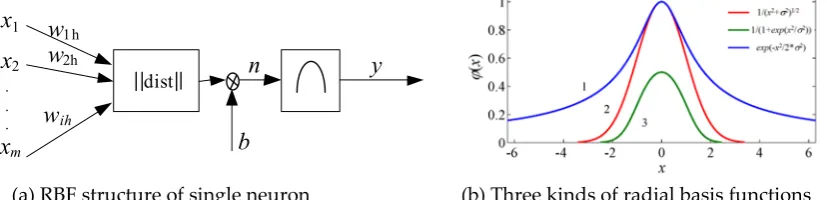
Figure 2 shows RBF structure of single neuron. The Euclidean distance between the input and the weight vector is used as the independent variable in RBF network. The activation function is generally Gauss's function, reflected sigmoidal function, inverse multiquadric function.
dist
w
2hw
ih· · ·
b
n
y
x
1w
1h
x
mx
2(a) RBF structure of single neuron (b) Three kinds of radial basis functions
The training data is classified correctly by a given hyperplane. Which is represented by (w,b). The hyperplane is equally expressed by all pairs
{
λ λw, b}
for λ∈R+. Thus, the canonical hyperplane is used to separate the data by a “distance”. The distance relationship satisfies the following formula:Gauss function:φ
( )
σ = − 2 2 exp 2 r
r (1)
Reflected Sigmoidal function: φ
( )
σ = + 2 2 1 1 exp r
r (2)
Inverse multiquadrics function:
( )
(
)
φ
σ =
+ 1/ 2
2 2
1
r r
(3)
σ is the expansion coefficient, the smaller the σ, the smaller the width of RBF, the more selective basis functions.
RBF network mainly needs three kinds of parameters: (1) Center of basis functions; (2) Expansion coefficient of basis function; (3) Weight of hidden layer and output layer.
2.1.1. Selection of Cluster Center
A variety of dynamic clustering algorithm is used to select the data center, the position of the data center should be adjusted in the process dynamically. K-means clustering algorithm is one of the common local search approaches, the advantage of the algorithm is that the expansion constant of each hidden node can be determined according to the distance between the cluster centers. Because the number of hidden nodes in RBF network has a great influence on its generalization ability, how to find a reasonable method to determine the number of clusters is a major task for the design of RBF network. Here, K-means algorithm is applied to determine the data center, the iterative procedure is shown in Equation (4).
η = − + = ( ) [ ( )] ( 1) ( )
i k i
i
i
t n X t n
t n
t n
= *
i i
else (4)
Where, ti is the i-th cluster center. ( )t ni is the i-th cluster center in iteration step n. (i=1,2,3,...,I). k
x is the k-th input sample. η is a learning factor. When t ni( + −1) t ni( ) <ξ, stop.
2.1.2. Determine the Expansion Coefficient
After determining the cluster center, the expansion coefficients of the corresponding radial basis functions can be determined according to the distance between the centers. Expansion coefficient σi
is represented in Equation (5).
= min − (5)
Where, Expansion coefficient = , is overlap coefficient.
2.1.3. Weight Factor
The output layer of the RBF network is a weighted sum of the hidden layer neurons. So the actual output of the RBF network is as follows:
( ) ( ) ( )
=Y n G n W n (6) Where,
Pseudo inverse method:
(7) = 1, k, NT
D d d d
D is expected value,G+ is a pseudo inverse matrix of matrix G.
( )
n
{
y
( )
n
}
k
N
j
J
Y
=
kj,
=
1
,
2
,
,
;
=
1
,
2
,
D
G
σ
= − − = =
,
2 2
1
exp 1, 2, ; 1, 2, ,
2
ki k i
i
g X t k N i I, (8)
{ }
= ij , =1, 2,, ; =1, 2,
W w i I j J
2.2. Annealed Chaotic Competitive Learning Network
2.2.1. Annealed Chaotic Function
The traditional neural network is probably not global-minima, but local-minima in the training process. So chaotic simulated annealing is used to escape from local-minima and get global-optimal solution by the annealed chaotic mechanism in neural network. The energy function of the neural network demonstrates the convergence process. The related research is proposed in [14–15]. A single chaotic dynamics neuron-annealing model is shown in eq.(9-10):
λ
− =
+ ( )/ 1 ( )
1 q t
p t
e (9)
μ
+ = − + − 0
( 1) ( ) ( )( ( ) I )
q t q t E T t p t (10) Where:
( )
p t = transient state of the interconnection strength between input neurons and output neurons ( )
q t = internal state of the interconnection strength between input neurons and output neurons 0
I = input bias for each neuron
μ = damping factor of nerve membrane(0≤ ≤μ 1)
E = energy function of the neural network λ = steepness factor of the output function(λ>0)
(t)
T = Self-feedback connection weight for input neurons and output neurons, (t)
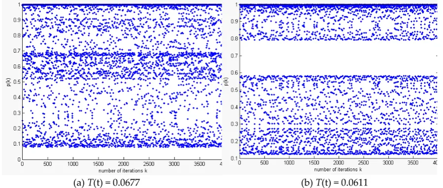
p is expressed by a value of the self-feedback connection weight ( )T t in equations (9) and (10). The various bifurcation states are demonstrated for the weight (t)T during 4000 iteration in Figure 3. The initial value of weight T is 0.0677. while T < 0. 0677, the transient state ( )p t shows a process from chaotic state though periodic bifurcation to a steady-state. The chaotic function converges with the decrease of ( )T t gradually. Where the initial condition is as follow: λ=0.004,
μ=0.899 , E=0, I0 =0.649. The chaotic behavior is used in a neural network. An annealed function is used to converge to a stable equilibrium point for a dynamic weight ( )T t .
(c) T(t) = 0.0533 (d) T(t) = 0.0328 Figure 3. Shows the various bifurcation states for different T(t) during 4000 iterations.
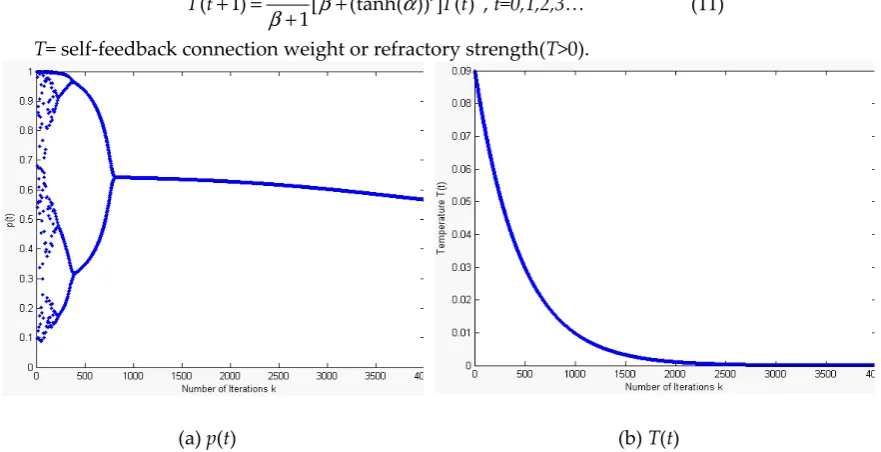
Figure 4 shows the time evolution of output ( )p t and annealing process ( )T t . The initial value for single neuron is as follows:E=0, I0=0.65, T0=0.09, λ=0.004 , μ=0.899 , α=0.9998,
β =450 [23]. ( )p t can converge to a steady-state value. It shows the process of a number of iterations and bifurcation of chaotic dynamics. Exponential damping of ( )T t is a process of simulated annealing [11]. The dynamic structure embeds into the competitive learning network in the experiment. Furthermore, the initial value of the parameters influences the dynamics process in training network. The above selected parameters are valid for all the bifurcation processes. The experiment shows the annealed chaotic mechanism can converge rapidly in the competitive network. Figure 4(a) demonstrates the output of a single neuron ( )p t . Figure 4(b) demonstrates annealing process of damping variable.
β α
β
+ = +
+ 1
( 1) [ (tanh( )) ] ( ) 1
t
T t T t , t=0,1,2,3… (11)
T= self-feedback connection weight or refractory strength(T>0).
(a) p(t) (b) T(t)
Figure 4. (a) Convergence process of single neuron p t( ); (b) Self-feedback connection weight T t( )
during 4000 iteration, or the damping variable corresponding to the temperature in the annealing process. (α =0.9998,β =450, E=0).
3. Proposed Method
collection, the EEG is polluted regularly by noise. The pure EEG is obtained by using thresholding of wavelet denoising method. (2) Feature extraction, the DWT is carried out on the EEG to get the sixth layer low frequency signal and the high frequency signal of the 2-6 layer, the δwave, θwave, αwave, β wave of EEG are selected by FFT and the sub-band energy is calculated. (3) Signal recognition, the neural network is used to recognize the EEG signal generated in different state.
Figure 5. The block diagram of EEG signal recognition. 3.1. Signal Processing
Figure 6 (a) shows that the raw EEG signal collected by sensor contain a large amount of noise, it will have a great impact on the subsequent feature extraction and recognition if it is not processed. The method based on the thresholding of wavelet denoising is shown in Figure 6 (b), the sym5 wavelet function is used to carry out the 5 layer decomposition of the raw EEG signal, the new
wavelet coefficients ^
, j k
W are get by thresholding based on equation (12) and (15). The pure EEG signal is shown in Figure 7 and the wavelet are restructured by using
^ , j k
W .
(a) (b)
Figure 6 (a)the raw EEG signal and (b)Pure EEG signal.
Figure 7 The wavelet denoising method based on thresholding.
The threshold selection is the key to identify noise and other details of the definition, in this paper the threshold T is obtained based on the method of Bayes Shrink threshold estimation:
δ δ δ
δ δ
δ δ
<
−
=
≥
2
2 2
2 2
2 2
max( , 0)
max(| |)
y y
n y
T
w
(12)
Where, wn is wavelet coefficients and δ is noise variance, the Median estimate is performed with the first layer of high frequency coefficient wHH:
k j
W , ~
k j
δ2= (1) 2
(Med w(| HH( , )|) / 0.6745)m n (13) δ2
y is energy estimation of each subband wavelet coefficients
δ
=
=
2 2
1 1 N
y n
n
w
N (14)
The threshold function is the different processing strategies to process wavelet coefficients above or below threshold T:
− ≥
=
<
( )(| |) 0 new
sign w w T w T
w
w T (15)
High frequency coefficients of noise correlation are filtered after threshold quantization, then the pure EEG signal are restructured based on the new coefficients wnew.
3.2. Feature Extraction
From the point of time domain, the EEG signals have no obvious feature, but feature is obvious and easy to get if time domain signal is transformed into frequency domain signal. The range of brainwave frequency changes greatly. Research shows that the frequency of brain activity is mainly between 0.5Hz and 40Hz and is shown in Table 1.
Table 1. Relationship between EEG frequency and brain states.
wave frequency(Hz) Activity description
δ 0.5~3 Extreme fatigue and deep sleep
θ 4~7 Suffer a setback or a mental depression
α 8~12 In quiet state and in a state of concentration
β 13~40 Nervous, emotional or excited state
EEG signal is a non-stationary signal, If the time domain signal is converted to the frequency domain by FFT, Its time domain information will be lost and the extracted features are too single, the processing effect is not very good. Here, The wavelet transform can obtain rich characteristics of EEG signal. The EEG signal is decomposed into different levels reconstruction signal by using db5 wavelet function and is shown in Figure 8. The FFT results of them are shown that they are similar to δ wave, θ wave, α wave, β wave of EEG. So we can obtain these waves by using wavelet transform method in Figure 9.
(a) (b)
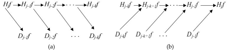
Figure 9. δ, θ, α, β wave based on wavelet transform. Signal decomposition expression:
φ ψ ∞ − − − =−∞ ∞ − − − =−∞ = − = −
1 1 1 1 1 1( ) (2 )
( ) (2 )
j j j k k j j j k k
H f x a x k
D f x d x k
(16)
Where detail coefficient: − − ∈ =
1 2 j j k l l k k Za h a detail coefficient: − − +
∈
=
−1
2 ( 1) j
i k
l k l
l k
k Z
d h a
scaling function: φ φ
∈
=
−( ) 2 k (2 ) k Z
x h x k
wavelet function: ψ φ
∈
=
−( ) 2 k (2 ) k Z
x g x k
Signal reconstruction expression:
φ ∞
=−∞
=
( ) j ( )
j k jk
k
H f x a x (17)
− −
− + −
∈ ∈
=
1+
− 12
2 ( 1)
j j k j
l k l
k k l l l
k Z k Z
a h a h d (18)
The raw data are decomposed by wavelet transform and obtain the δ(x) wave, θ(x) wave, α(x) wave, β(x) wave, its sub-band signal energy is shown as follows:
δ
δ =
=
21 1
( ) ( ( )) N
n
E X N
N (19)
θ
θ =
=
21 1
( ) ( ( )) N
n
E X N
N (20)
α
α =
=
21 1
( ) ( ( )) N
n
E X N
N (21)
β
β =
=
21 1
( ) ( ( )) N
n
E X N
N (22)
Calculate the energy ratio of each signal:
Eall= E(δ) + E(θ) + E(α) + E(β) (23)
En(δ) = E(δ)/Eall (24)
En(α) = E(α)/Eall (26)
En(β) = E(β)/Eall (27)
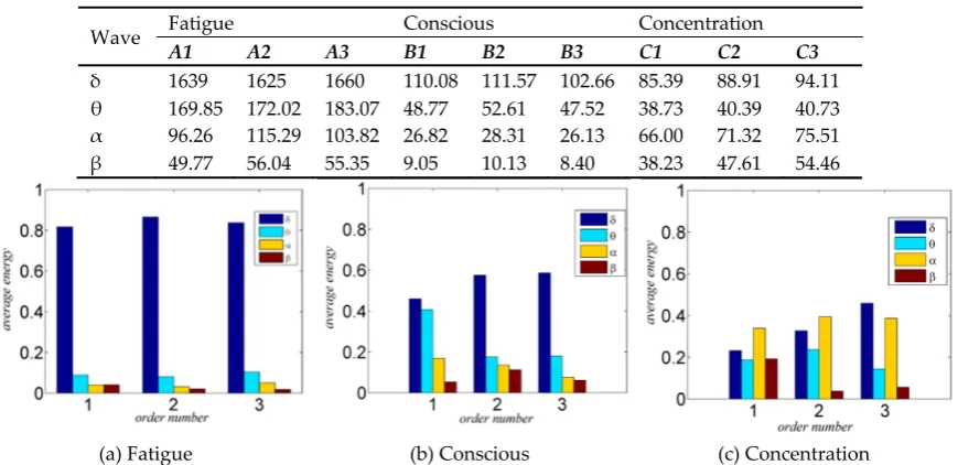
The energy values in Table 2 are normalized by the formula (23-27) and the results are shown in Figure 10, In fatigue state, the sub-band energy of EEG signal is mainly focused on the δ wave; In the conscious state, the energy of δ wave decreases, and the other wave energy rises; In a concentrated state, the energy of α wave is more prominent. for the frequency, with the concentration of the mental state, the energy of the low frequency signal is reduced, and the energy of the high frequency signal is increased. After wavelet decomposition, the ratio of EEG signals in different states can be quantitatively analyzed, The extracted features are obvious and easy to be distinguished, which lays the foundation for the accurate and reliable identification of neural networks.
Table 2 The average energy value in the different states
Wave Fatigue Conscious Concentration
A1 A2 A3 B1 B2 B3 C1 C2 C3 δ 1639 1625 1660 110.08 111.57 102.66 85.39 88.91 94.11 θ 169.85 172.02 183.07 48.77 52.61 47.52 38.73 40.39 40.73 α 96.26 115.29 103.82 26.82 28.31 26.13 66.00 71.32 75.51 β 49.77 56.04 55.35 9.05 10.13 8.40 38.23 47.61 54.46
(a) Fatigue (b) Conscious (c) Concentration
Figure 10 Energy distribution in the different states.
3.3. Annealed Chaotic Competitive Learning Network
The conventional competitive learning network may be obtained local minimum solutions in the training network, thus embeds into an annealed chaotic mechanism and obtains an optical solution in a global scope for the network [17]. The transient chaotic network model sensitively relies on a self-feedback connection weight. The weight is similar to a stochastic simulated annealing temperature and changes dynamically in the process of the network. The annealed chaotic competitive network can escape the local-minima and reduce the convergence time quickly.
Figure 11. Chaotic annealing mechanism embedded in the ACCLN network topology.
The convergence process of the ACCLN is shown in [18]. The neuron states are changed by the function qx j; . A simulated annealing strategy is used as the training network by Equation (28). The network model has n neurons in the input layer, c neurons in the output layer and n × c
interconnection strengths. The mathematical expression of this model is shown as follows:
= =
=
; − 21 1 1 2
n c
x j x j x j
E p z w (28)
λ
− =
+ ;
; ( )/
1 ( )
1 x j
x j q t
p t
e (29) μ
+ = + − −
;( 1) ;( ) ( )( ; ( ) I )0
x j x j x j
q t q t E T t p t (30) η
= −
wj (zx w )j px j; (31)
β α
β
+ = +
+ 1
( 1) [ (tanh( )) ] ( ) 1
t
T t T t (32)
+ = +
( 1) ( ) ( )
j j j
w t w t w t (33)
Where Eis energy function, the network has n input neuron nodes and c output nodes. px j;
and qx j; are the transient state and internal state of interconnection strength, respectively. wj is weight coefficient between each input neuron node and output neuron node. η is a small learning-rate parameter. These parameters are updated in real time in training process.
4. Experiment
4.1. The Experimental Platform and EEG Signal Extraction
(a)Electrode position (b) Subjects Figure 12. EEG acquisition and electrode position.
30 subjects are selected in the experiment, 10 people who slept for 12 hours are regarded as conscious subjects, 10 people who are not sleeping for 12 hours are regarded as fatigue subjects. 10 people who are playing game after sleeping for 12 hours are regarded as concentration subjects.
Neural network is an adaptive pattern recognition technology, it does not need to give the empirical knowledge and discriminant function, which can train the information from different states and obtain some kind of mapping relation. Therefore, neural networks have been widely used in pattern recognition, The identification process is shown in Figure 13.
Figure 13. System structure based on neural network.
4.2. Test Experiment Based on RBF Network
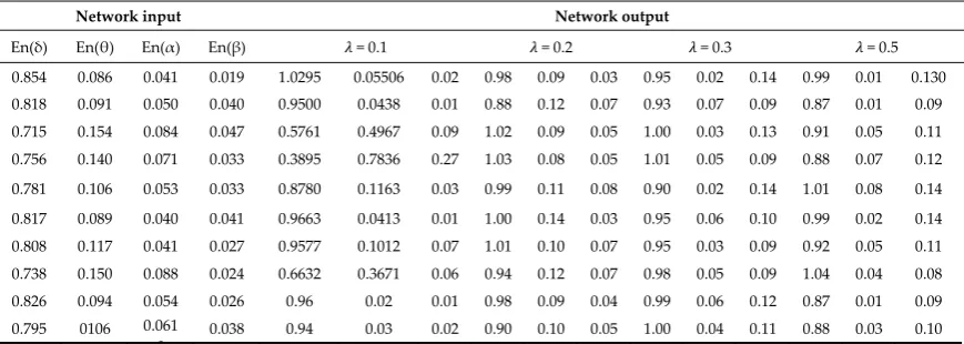
Set the overlap coefficient of RBF network is 0.1,0.2,0.3,0.5. Feature (Eδ,Eθ,Eα,Eβ) is
extracted from 500 sets of acquisition data sample and is regarded as training sample. 100 sets of EEG signals of the subjects are acquired in fatigue, conscious and concentration state. The feature vector is calculated as the input of the neural network. In three different states, the classification results of the 10 sets of test samples are shown in the Table 3–5.
Table 3. The RBF network output with different overlap coefficient under fatigue state.
Network input Network output
En(δ) En(θ) En(α) En(β) = 0.1 = 0.2 = 0.3 = 0.5
0.854 0.086 0.041 0.019 1.0295 0.05506 0.02 0.98 0.09 0.03 0.95 0.02 0.14 0.99 0.01 0.130
0.818 0.091 0.050 0.040 0.9500 0.0438 0.01 0.88 0.12 0.07 0.93 0.07 0.09 0.87 0.01 0.09
0.715 0.154 0.084 0.047 0.5761 0.4967 0.09 1.02 0.09 0.05 1.00 0.03 0.13 0.91 0.05 0.11
0.756 0.140 0.071 0.033 0.3895 0.7836 0.27 1.03 0.08 0.05 1.01 0.05 0.09 0.88 0.07 0.12
0.781 0.106 0.053 0.033 0.8780 0.1163 0.03 0.99 0.11 0.08 0.90 0.02 0.14 1.01 0.08 0.14
0.817 0.089 0.040 0.041 0.9663 0.0413 0.01 1.00 0.14 0.03 0.95 0.06 0.10 0.99 0.02 0.14
0.808 0.117 0.041 0.027 0.9577 0.1012 0.07 1.01 0.10 0.07 0.95 0.03 0.09 0.92 0.05 0.11
0.738 0.150 0.088 0.024 0.6632 0.3671 0.06 0.94 0.12 0.07 0.98 0.05 0.09 1.04 0.04 0.08
0.826 0.094 0.054 0.026 0.96 0.02 0.01 0.98 0.09 0.04 0.99 0.06 0.12 0.87 0.01 0.09
0.795 0106 0.061 0
Table. 4 The RBF network output with different overlap coefficient under conscious state
Network input Network output
En(δ) En(θ) En(α) En(β) = 0.1 = 0.2 = 0.3 = 0.5
0.460 0.408 0.170 0.053 0.1564 0.6829 0.5008 0.02 0.93 0.03 0.04 1.02 0.05 0.03 0.95 0.10
0.575 0.176 0.135 0.112 0.0011 1.0270 0.0339 0.04 0.92 0.05 0.03 0.97 0.15 0.01 0.95 0.04
0.587 0.180 0.177 0.061 0.0118 0.9206 0.0762 0.03 1.03 0.08 0.02 0.95 0.07 0.04 0.96 0.10
0.601 0.162 0.146 0.091 0.0311 0.9595 0.0121 0.03 1.04 0.03 0.02 0.967 0.03 0.02 1.02 0.12
0.559 0.217 0.153 0.071 0.0132 1.0089 0.0116 0.00 0.98 0.14 0.02 0.93 0.15 0.01 0.92 0.03
0.489 0.321 0.110 0.089 0.0168 1.0530 0.0244 0.01 0.98 0.03 0.01 0.93 0.13 0.04 0.92 0.02
0.562 0.211 0.144 0.083 0.0086 1.0288 0.0271 0.03 0.96 0.03 0.02 1.04 0.07 0.04 0.94 0.05
0.511 0.387 0.074 0.028 0.0254 1.0637 0.1527 0.04 1.03 0.02 0.01 1.04 0.01 0.020 1.00 0.05
0.482 0.233 0.186 0.112 0.0254 1.0637 0.1527 0.04 0.96 0.03 0.02 0.99 0.04 0.03 1.01 0.07
0.510 0.221 0.165 0.104 0.1235 1.0145 0.0189 0.03 0.93 0.07 0.02 0.92 0.06 0.02 0.97 0.08
Table 5 The RBF network output with different overlap coefficient under concentrated state
Network input Network output
En(δ) En(θ) En(α) En(β) = 0.1 = 0.2 = 0.3 = 0.5
0.232 0.187 0.339 0.192 0.0186 0.074 0.9576 0.03 0.04 0.88 0.00 0.12 1.09 0.05 0.06 0.86
0.327 0.237 0.395 0.038 0.0024 0.041 0.9973 0.06 0.12 0.92 0.03 0.10 0.99 0.06 0.09 1.07
0.459 0.144 0.387 0.056 0.0235 0.096 1.1001 0.04 0.04 1.05 0.01 0.16 0.98 0.06 0.14 1.07
0.428 0.167 0.351 0.054 0.0156 0.004 0.9853 0.04 0.04 0.86 0.06 0.12 0.91 0.02 0.11 1.05
0.451 0.151 0.264 0.132 0.0215 0.348 0.7210 0.06 0.10 1.08 0.05 0.14 0.97 0.04 0.04 0.88
0.506 0.196 0.264 0.032 0.0282 0.444 0.6040 0.05 0.06 1.03 0.03 0.09 1.00 0.01 0.09 0.92
0.410 0.220 0.304 0.065 0.0785 0.211 0.8609 0.04 0.14 0.97 0.03 0.09 1.02 0.00 0.10 0.94
0.285 0.229 0.322 0.162 0.0797 0.178 0.9283 0.01 0.14 0.99 0.00 0.09 0.95 0.05 0.09 1.02
0.318 0.189 0.353 0.14 0.0315 0.145 0.9541 0.01 0.13 0.97 0.04 0.14 0.94 0.03 0.12 0.89
0.353 0.176 0.332 0.13 0.0035 0.134 0.9721 0.06 0.05 0.91 0.05 0.05 1.09 0.03 0.07 1.03
The expected output of the network is (0, 1, 0) under the fatigue state, the conscious state is (1, 0, 0), and the concentration state is (0, 0, 1). The output function of the RBF network is a linear function and the output range is [0, 1]. Root mean square error is calculated by formula (34). The closer the actual output and the expected output is, the more accurate the test is. Figure 14 shows the error of RBF network in different state. When the overlap coefficient is 0.1, the recognition effect is the worst, and the partial difference is more than 0.5, With the increase of , the higher the accuracy rate of RBF network, the smaller the output error.
(a) the fatigue state (b) the conscious state (c) the concentrated state
Figure 14 Output error of RBF network
(34)
50
)
(
RMSE
501
2
=
−
=
nA T
v
Table 6.The correct recognition rate of EEG signal based on RBF network.
Fatigue Conscious Concentration
=0.1 =0.2 =0.3 =0.5 =0.1 =0.2 =0.3 =0.5 =0.1 =0.2 =0.3 =0.5
Accuracy 85% 88% 89% 93% 84% 88% 87% 94% 85% 87% 89% 93%
EMSE 0.263 0.089 0.061 0.037 0.249 0.075 0.066 0.032 0.256 0.085 0.080 0.034
4.3. ACCLN Experiment
The same training sample is used to train the ACCLN network. That’s to say, the data includes 500 sets of training samples and 100 sets of testing samples in the experiment. In three different states, the classification results of the 10 sets of test samples are shown in Table 7–9.
Table 7. The ACCLN network output under fatigue state.
Network input Network output
En(δ) En(θ) En(β) En(β) V1 V2 V3
1 0.854 0.086 0.041 0.019 1 0 0
2 0.818 0.091 0.050 0.040 1 0 0
3 0.715 0.154 0.084 0.047 1 0 0
4 0.756 0.140 0.071 0.033 1 0 0
5 0.781 0.106 0.053 0.033 1 0 0
6 0.817 0.089 0.040 0.041 1 0 0
7 0.808 0.117 0.041 0.027 1 0 0
8 0.738 0.150 0.088 0.024 1 0 0
9 0.826 0.094 0.054 0.026 1 0 0
10 0.795 0106 0.061 0.038 1 0 0
Table 8. The ACCLN network output under conscious state.
Network input Network output
En(δ) En(θ) En(α) En(β) V1 V2 V3
1 0.460 0.408 0.170 0.053 0 1 0
2 0.575 0.176 0.135 0.112 0 1 0
3 0.587 0.180 0.177 0.061 0 1 0
4 0.601 0.162 0.146 0.091 0 1 0
5 0.559 0.217 0.153 0.071 0 1 0
6 0.489 0.321 0.110 0.089 0 1 0
7 0.562 0.211 0.144 0.083 0 1 0
8 0.511 0.387 0.074 0.028 0 1 0
9 0.482 0.233 0.186 0.112 0 1 0
10 0.510 0.221 0.165 0.104 0 1 0
Table 9 Table 8 The ACCLN network output under concentrated state.
Network input Network output
En(δ) En(θ) En(α) En(β) V1 V2 V3
1 0.232 0.187 0.339 0.192 0 0 1
2 0.327 0.237 0.395 0.038 0 0 1
3 0.459 0.144 0.387 0.056 0 0 1
4 0.428 0.167 0.351 0.054 0 0 1
5 0.451 0.151 0.264 0.132 0 0 1
6 0.506 0.196 0.264 0.032 0 0 1
7 0.410 0.220 0.304 0.065 0 0 1
8 0.285 0.229 0.322 0.162 0 0 1
9 0.318 0.189 0.353 0.140 0 0 1
The output function of the ACCLN has only two states, 0 or 1. That’s to say, the recognition result is true or false. Compared with RBF network, the correct recognition rate of ACCLN network is high. the number of the correct identification is 97 in the fatigue state, 98 in conscious state and 97 in a concentrated state. In the test samples of the 300 groups, the recognition error is 7, and the success rate is 97.6%. In general, brainwave recognition rate of ACCLN network is superior to the RBF network.
5. Conclusions
In this paper, a new method is proposed that recognition method of EEG signals uses discrete wavelet transform and neural network. First of all, the raw EEG signals are acquired by headset of NeuroSky Inc.. Because of the noise in the signal acquisition and transmission, it is necessary to remove the noise. Wavelet denoising method based on threshold is a good way of removing the high frequency noise of the signal. And then, the δ wave, θ wave, α wave, β wave of EEG signals are obtained by DWT and FFT, the energy value of different wave is used as the characteristic value of the signal recognition. Finally, the ACCLN network and RBF neural network with different overlap coefficient are used to identify the EEG signal, the experiment result shows that ACCLN network is a better way to recognize EEG signals than RBF network, At the same time, the effectiveness of the proposed algorithm is verified, which lays a good foundation for the subsequent development of BCI technology.
Acknowledgments: The authors are grateful for the support from the Industrial Science and technology research foundation of Shaanxi province, No. 2015GY020 and foundation of Shaanxi Educational Committee No. 15JK1472.
Author Contributions: Xuebin Qin and Jun Deng conceived and designed the experiments; Yizhe Zhang and Pai Wang performed the experiments; Xuebin Qin and Mei Wang analyzed the data; Yizhe Zhang contributed EEG data; Xuebin Qin wrote the paper.
Conflicts of Interest: The authors declare that there is no conflict of interest regarding the publication of this paper.
References
1. T. Yohei,I. F. Benoit, and D. Gerard. “Bimodal BCI using simultaneously NIRS and EEG,” IEEE Transl. J. Biomedical Engineering, 2014, 61(4), pp. 1274-1284
2. V. Ivan, R. B. Pachori, L. Thorsten, M. Malechka, Tatsiana,and G. Axel,“BCI demographics II: How many (and What Kinds of) people can use a high-frequency SSVEP BCI,” IEEE Trans. J. Neural Syst. Rehabil. Eng, 2011, 19(3), pp.232-239
3. K. Rafal1, V. Diana, Z. Jaroslaw, M. Tatsiana, G. Axel, and D. Piotr, “Asynchronous BCI based on motor imagery with automated calibration and neurofeedback training,” IEEE Transl. J. Neural Syst Rehabil. Eng, 2012, 20(6), pp. 823-825
4. A. H. Zhang, and Y. Feng, “EEG feature extraction and analysis under drowsy state based on energy and sample entropy,”2012 5th International Conference on Biomedical Engineering and Informatics, BMEI, 2012, pp. 501-505
5. N. Viswam, and J. Roozbeh, “Reducing the noise level of EEG signal acquisition through reconfiguration of dry contact electrodes,” IEEE 2014 Biomedical Circuits and Systems Conference, BioCAS, 2014, pp. 572-575
6. M. B. Hamaneh, N. Chitravas,K. Kaiboriboon, S. Lhatoo, and K. A. Loparo, “Automated removal of EKG artifact from EEG data using independent component analysis and continuous wavelet transformation,” 2014, IEEE Trans. J. BE, 61(6), pp. 1634-1641
7. L. Zhu, Z.Gu, and Y. Li, “Grouped Automatic Relevance Determination and Its Application in Channel Selection for P300 BCIs,” 2015, IEEE Transl. J. NEUR SYS REH, 23(6) pp. 1068-1077
9. H. Higashi,and T. Tanaka, “Simultaneous design of FIR filter banks and spatial patterns for EEG signal classification,” 2013, IEEE Trans. J. BE, 60(4), pp. 1100-1110
10. M. A. Lopez-Gordo, F. Pelayo, and E. Fernandez, “Fernandez E. Phase-shift keying of EEG signals: Application to detect attention in multitalker scenarios,” J. Signal Processing, 2015, pp. 165-173
11. Musha, Toshimitsu, and Matsuzaki,“EEG markers for characterizing anomalous activities of cerebral neurons in NAT (neuronal activity topography) method,” IEEE Transl. J. Biomedical Engineering, 2013, 60(8), pp. 2332-2338
12. Z. Christoph, T.Johannes, and Z. Carl,“Brain-state dependent brain stimulation: Real-time EEG alpha band analysis using sliding window FFT phase progression extrapolation to trigger an alpha phase locked TMS pulse with 1 millisecond accuracy,” J. Brain Stimulation, 2015, 8(2), pp. 378-389.
13. Liu Ying, J. Moser, and S. Aviyente, “Network community structure detection for directional neural networks inferred from multichannel multisubject EEG data,” IEEE Transl. J. Biomedical Engineering, 2014, 71(7), pp. 1919-1930.
14. George, A.; Katerina, T. Simulating annealing and neural networks for chaotic time series forecasting. Chaotic Model. Simul. 2012, pp. 81–90
15. Atsalakis, G.; Skiadas, C. Forecasting Chaotic time series by a Neural Network. In Proceedings of the 8th International Conference on Applied Stochastic Models and Data Analysis, Vilnius, Lithuania, 30 June–3 July 2008; pp. 77–82
16. Liu, H.; Li, S. Decision fusion of sparse representation and support vector machine for SAR image target recognition. Neurocomputing 2013, 113, 97–104.
17. Zhang, J.-M.; Liang, S. Research on Fault Location of Power Cable with Wavelet Analysis. In Proceedings of the IEEE Digital Manufacturing and Automation, Hunan, China, 5–7 August 2011; pp. 956–959. 18. Lin, J.-S. Annealed chaotic neural network with nonlinear self-feedback and its application to clustering
problem. Patten Recognition. 2001, 34(2), pp.1093–1104