Theses and Dissertations
2015
Drilled Shaft Skin Resistance Design in the Cooper
Marl
William J. Gieser University of South Carolina
Follow this and additional works at:https://scholarcommons.sc.edu/etd Part of theCivil Engineering Commons
This Open Access Thesis is brought to you by Scholar Commons. It has been accepted for inclusion in Theses and Dissertations by an authorized administrator of Scholar Commons. For more information, please [email protected].
Recommended Citation
by
William J. Gieser
Bachelor of Science
Georgia Institute of Technology, 2009
Submitted in Partial Fulfillment of the Requirements
For the Degree of Master of Science in
Civil Engineering
College of Engineering and Computing
University of South Carolina
2015
Accepted by:
Sarah L. Gassman, Director of Thesis
Charles E. Pierce, Reader
To my grandfather, Herbert P. Gieser, who always believed in hard work and
Throughout the process of research and writing, I have received a lot of help
along the way. I would first like to thank all the teachers who have taught me along the
way from kindergarten until the last class I took at the University of South Carolina.
Every one of you has contributed something that helped in this task. For my time at the
University of South Carolina, I would like to thank Dr. Chunyang Liu, Dr. Nathan
Huynh, Dr. Nicole Berge, Dr. Michelle Maher, Dr. Charles Pierce, and Dr. Mike
Meadows. All of you taught me while I was at the university and I truly appreciate it. In
particular, I would also like to thank Dr. Sarah Gassman who was my academic advisor
and thesis advisor in addition to a class professor. I really appreciate your patience with
me throughout this process and your willingness to answer as many questions as it took
for me to learn in the four classes you taught me as well as the thesis work.
In the preparation of this thesis, I would like to thank Zane Abernethy for helping
me with the engineering logic and local engineering and construction history, James
“Ricky” Wessinger and Dr. Will Doar, III for helping with the geologic research and
review, and Chris Gaskins and Jon Sinnreich for providing me with the load test data
used in the analysis. Without all of you, this research would not have been possible.
Finally, but not least, I would like to thank my friends and family for their support
through the entire graduate school process. Sometimes, someone telling you that you
As drilled shafts have become a more popular foundation type in the Charleston,
South Carolina area, there has been an ongoing goal of optimizing drilled shaft design
while maintaining the structural integrity of the foundation. In the Charleston area, the
primary bearing stratum for deep foundations is the Cooper Marl, a calcareous Oligocene
formation. Research performed from 2002 to 2004 on load test data from drilled shafts
constructed in the Cooper Marl and soil properties from three test sites for the Cooper
River Bridge explored the relationship between the measured skin resistance and
geotechnical properties. In the 15 years since the load tests for the Cooper River Bridge
were performed, additional load tests have been performed throughout the Charleston
area. Evaluation of this load test data, the Cooper River Bridge load test data, and earlier
load test data allows better understanding of drilled shaft skin resistance in the Cooper
Marl as well as the ability to use in-situ geotechnical properties to better predict axial
capacity when a load test is not performed. Drilled shafts founded in the Cooper Marl are
designed primarily for using skin resistance and LRFD design methodologies and load
factors.
Using data from 27 drilled shaft load tests at 15 test sites in the Cooper Marl, the
relationships between load test measured unit skin resistance and undrained shear
strength, overburden pressure, and SPT N-values were evaluated. The distribution of unit
skin resistance with elevation was also studied across the Cooper Marl. To derive a
Finally, an empirical method was used to verify the LFRD resistance factor currently
required for design in the Cooper Marl.
Based on the performed analyses, there is not a correlation between unit skin
resistance and SPT N-values. Across the Cooper Marl, the unit skin resistance
distribution was found to be constant with depth up to -80 ft-MSL. When evaluating the
relationship between undrained shear strength and unit skin resistance, the α-value was found to be 0.85, which is approximately 60% larger than the α values for clay presented in the literature. Based on the load test data, a design unit skin resistance of 3.2 ksf is
supported using the historical load test method and a unit skin resistance of 2.88 ksf is
supported using the 97.5% confidence interval method for typical sites. Additionally, the
current resistance factor for LRFD design of 0.45 is data supported. Finally, although the
Cooper Marl is treated as a homogeneous formation, there are known geologic
DEDICATION ... iii
ACKNOWLEDGEMENTS ... iv
ABSTRACT ...v
LIST OF TABLES ...x
LIST OF FIGURES ... xi
LIST OF SYMBOLS ... xiv
LIST OF ABBREVIATIONS ... xvi
CHAPTER 1:INTRODUCTION ...1
1.1PURPOSE OF RESEARCH ...1
1.2RESEARCH QUESTIONS ...3
1.3DOCUMENT ORGANIZATION ...4
CHAPTER 2:LOCAL GEOLOGY ...5
2.1INTRODUCTION ...5
2.2COOPER MARL GEOLOGICAL HISTORY AND GEOLOGIC CLASSIFICATION ...5
2.3COOPER MARL GEOGRAPHICAL DISTRIBUTION ...6
2.4COOPER MARL PHYSICAL PROPERTIES ...12
2.5COOPER MARL DISCONTINUITIES AND ANOMALIES ...14
CHAPTER 3:BACKGROUND ...17
3.1INTRODUCTION ...17
3.4DRILLED SHAFT VERIFICATION TESTING ...21
3.5EFFECTS OF DRILLED SHAFT DEFECTS ON AXIAL PERFORMANCE ...23
3.6DRILLED SHAFT LOAD TESTING INFORMATION ...24
3.7TYPES OF DRILLED SHAFT LOAD TESTS ...26
3.8LOAD TEST INTERPRETATION ...34
3.9DRILLED SHAFT AXIAL DESIGN ...44
CHAPTER 4:DATA ...59
4.1LOAD TEST DATA ...59
4.2CONSTRUCTION INFORMATION ...62
4.3SPTDATA ...64
4.4LAB TEST DATA ...67
4.5LOAD TEST RESULTS ...67
4.6DATA SORTING FOR ANALYSIS ...71
CHAPTER 5:METHODOLOGY ...76
5.1INTRODUCTION ...76
5.2RELATIONSHIP BETWEEN SKIN RESISTANCE AND GEOTECHNICAL PROPERTIES ..76
5.3DESIGN SKIN RESISTANCE ...79
5.4AXIAL RESISTANCE FACTOR ...81
5.5ANALYSIS ASSUMPTIONS ...83
CHAPTER 6:DATA ANALYSIS ...86
6.1INTRODUCTION ...86
6.2SKIN RESISTANCE VERSUS SPTN-VALUES ...86
6.5RELATIONSHIP OF SKIN RESISTANCE TO UNDRAINED SHEAR STRENGTH ...95
6.6LOAD TEST SKIN RESISTANCE DISTRIBUTION ...96
6.7STATISTICALLY BASED UNIT SKIN RESISTANCE...102
6.8HISTORICAL LOAD TEST METHOD BASED UNIT SKIN RESISTANCE ...103
6.9DESIGN UNIT SKIN RESISTANCE RECOMMENDATIONS ...104
6.10GEOTECHNICAL RESISTANCE FACTORS IN THE COOPER MARL ...105
CHAPTER 7:CONCLUSIONS ...107
7.1INTRODUCTION ...107
7.2CONCLUSIONS ...107
7.3FUTURE RESEARCH PATHS ...112
WORKS CITED ...113
Table 3.1 Methods for Evaluating the α-Value ...48
Table 3.2 Predicted Skin Resistance Compared to Measured Skin Resistance ...51
Table 3.3 Drilled Shaft Resistance Factors, φ ...53
Table 4.1 Summary of Available Drilled Shaft Load Test Data ...61
Table 5.1 Constants for Becker (2005) Resistance Factor Equation ...82
Table 5.2 Unit Skin Resistance by Load Test Type ...84
Table 6.1 R2 Values for the SPT to Unit Skin Resistance Relationship ...91
Table 6.2 Average Unit Skin Resistance in the Cooper Marl ...95
Table 6.3 Statistical Information of the Unit Skin Resistance Distribution for Data Set 1 ...98
Table 6.4 Statistical Information of the Unit Skin Resistance Distribution for Data Set 2 ...100
Table 6.5 Statistical Information of the Unit Skin Resistance Distribution for Data Set 3 ...102
Table 6.6 Minimum and 97.5% Exceeding Values for All Data Sets ...102
Table 6.7 Statistically Derived Unit Skin Resistance Values for All Data Sets ...103
Table 6.8 Historical Load Test Method Derived Skin Resistance Values ...104
Figure 2.1 Excerpt of Cross-Section C-C’ from Lexington to Charleston ...8
Figure 2.2 Stratigraphic Units Directly Underlying Quaternary Cover in the Charleston, SC Region ...11
Figure 2.3 Contour Map of the Base of the Ashley Formation in the Charleston, SC Region ...12
Figure 2.4 Undrained Shear Strength of the Cooper Marl at the Cooper River Bridge ....13
Figure 2.5 Contour Map of the Base of the Marks Head Formation in the Charleston, SC Region ...16
Figure 3.1 Conventional Method Load Test ...27
Figure 3.2 Typical Osterberg Cell Setup ...29
Figure 3.3 Statnamic Load Test Setup and Sequence ...31
Figure 3.4 Example of a Load versus Displacement Graph ...35
Figure 3.5 Example of a Load versus Depth Graph ...37
Figure 3.6 Example of an Osterberg Equivalent Top Load-Displacement Graph ...38
Figure 3.7 Example of an Osterberg Load Test Load versus Depth Graph ...39
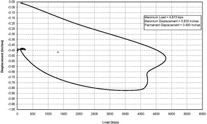
Figure 3.8 Example of a Statnamic Load versus Displacement Graph ...41
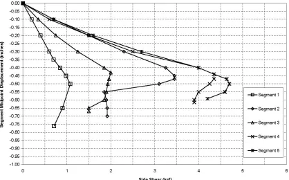
Figure 3.9 Example of a Unit Side Shear versus Displacement Graph ...42
Figure 3.10 Example of a Load versus Displacement Graph for an APPLE Test ...43
Figure 4.1 Location Map of Load Tests ...60
Figure 4.2 Test Shaft Schematic Drawing ...63
Figure 4.5 Example Load Test Report Skin Resistance Table from Test Site 15 ...68
Figure 4.6 Load Test Skin Resistance Distributions ...69
Figure 6.1 Field N-Values versus Unit Skin Resistance for Data Set 1 ...87
Figure 6.2 N60 Values versus Unit Skin Resistance for Data Set 1 ...87
Figure 6.3 Field N-Values versus Unit Skin Resistance for Data Set 2 ...88
Figure 6.4 N60 Values versus Unit Skin Resistance for Data Set 2 ...88
Figure 6.5 Field N-Values versus Unit Skin Resistance for Data Set 3 ...89
Figure 6.6 N60 Values versus Unit Skin Resistance for Data Set 3 ...89
Figure 6.7 Field N-Values versus Unit Skin Resistance for Data Set 3 Sorted by Load Test Type ...90
Figure 6.8 N60 Values versus Unit Skin Resistance for Data Set 3 Sorted by Load Test Type ...90
Figure 6.9 Unit Skin Resistance in the Cooper Marl versus Elevation for All Test Sites .92 Figure 6.10 Effective Overburden Pressure versus Unit Skin Resistance for Data Set 1 ..93
Figure 6.11 Effective Overburden Pressure versus Unit Skin Resistance for Data Set 2 ..94
Figure 6.12 Effective Overburden Pressure versus Unit Skin Resistance for Data Set 3 ..94
Figure 6.13 Frequency Distribution of Unit Skin Resistance Based on One Foot Increments for Data Set 1 ...97
Figure 6.14 Frequency Distribution of Unit Skin Resistance Based on a Per Site Basis for Data Set 1...97
Figure 6.15 Frequency Distribution of Unit Skin Resistance Based on One Foot Increments for Data Set 2 ...99
Figure 6.16 Frequency Distribution of Unit Skin Resistance Based on a Per Site Basis for Data Set 2...99
A Shaft segment surface area
B Shaft diameter
COV Coefficient of variation
DL Dead load
FS Factor of safety
fs Unit skin resistance
fSN Nominal unit side resistance
LL Live load
Kr Ratio of mean value to characteristic value
N60 N-value corrected for hammer energy ratio
Pa Atmospheric pressure
Q Total load / allowable working load / factored load
QD Nominal value of dead load
QL Nominal value of live load
Qi Unfactored axial load
R2 Coefficient of determination
Rn Nominal resistance
Rr Factored resistance
RSN Nominal side resistance
α Skin resistance coefficient
β Reliability index
γD Mean of the bias values for the dead load
γDL Load factor for dead load
γi Load factor
γLL Load factor for live load, mean of the bias values for the live load
γR Mean of the bias values for resistance
Δz Thickness of soil layer
ηi Load modifier
θ Separation coefficient
AASHTO ... American Association of State Highway and Transportation Officials
ASD... Allowable Stress Design
ASTM ... American Society for Testing and Materials
bpf ... Blows per Foot
CAPWAP ... Case Pile Wave Analysis Program
CPT ... Cone Penetration Test
CSL ...Cross-hole Sonic Logging
FAT ... First Arrival Time
FHWA ... Federal Highway Administration
ft-MSL... Feet – Mean Sea Level
GDM ... Geotechnical Design Manual
ksf ... Kips per Square Foot
LRFD ... Load and Resistance Factored Design
pcf ... Pounds per Cubic Foot
psi ... Pounds per Square Inch
PDA... Pile Driving Analyzer
PIT... Pile Integrity Test
SCDOT ... South Carolina Department of Transportation
SPT ... Standard Penetration Test
TIP... Thermal Integrity Profiling
CHAPTER 1
INTRODUCTION
1.1 - Purpose of Research
As drilled shafts have become a more popular foundation type in the Charleston,
South Carolina area, there has been an ongoing goal of optimizing drilled shaft design
while maintaining the structural integrity of the foundation. An effective method of
optimizing drilled shaft length is by performing a drilled shaft load test at the
construction site to verify the design parameters used to represent the underlying soils. In
the Charleston area, the primary bearing stratum is the Cooper Marl, a calcareous
sedimentary deposit. This stratum is an Oligocene age formation that is only found in the
coastal plain of South Carolina and is primarily concentrated in the Charleston area.
Currently, the South Carolina Department of Transportation (SCDOT) uses Load
and Resistance Factored Design (LRFD) methods for drilled shaft analysis and design.
This design method applies a geotechnical resistance factor to the expected shaft
resistance to account for geotechnical uncertainty and construction defects. LRFD allows
for a reduced geotechnical resistance factor for sites where a load test is performed, as a
load test reduces the geotechnical uncertainty. However, as load tests are relatively
expensive, this is not a feasible option for smaller bridges. For these smaller bridges,
empirical design methods or load test results from similar sites are used to represent
design foundation resistance. However, these two methods require the use of a higher
additional geotechnical uncertainty. The reduction in the geotechnical resistance factor
provided by load testing allows for drilled shafts to be shorter as the load test reduces the
uncertainty in the geotechnical resistance. Because of this, knowledge of geotechnical
resistance is critical to optimizing drilled shaft design and, in turn, maximizing cost
savings.
Existing load test data, geotechnical field investigations, and knowledge of the
area geology can be utilized to better define the expected soil behavior for drilled shaft
construction. The primary goal of this thesis is to provide design engineers with data and
analysis that will help improve the design of drilled shaft supported bridges where load
tests are not performed and improve the preliminary design of bridges where load tests
will be performed. This will be accomplished by evaluating the relationship between
load test measured resistance and its correlation to in-situ testing, compiling load test data
to derive data-supported soil resistance values in the Cooper Marl, and seeing if the
geotechnical resistance factors that are used for drilled shaft construction, which are
based on load tests in many soil formations, are applicable in the Cooper Marl. Some
previous research into these topics has been performed, with the majority of the data
coming from the Cooper River Bridge test sites. This included research into the effects of
construction techniques on skin resistance, the effect of vertical effective stress on skin
resistance, and comparing multiple empirical methods for estimating skin resistance to
load test measured skin resistance. Currently, the majority of bridge foundation designs
in this area that do not involve load testing are based on area specific common
Previous research conducted by Camp (2004) on the relationship between vertical
effective stress and skin resistance, which did not show a direct correlation to unit skin
resistance. However, there is limited information regarding the relationship between
in-situ testing and unit skin resistance, with most of the relationships being based on testing
at the Cooper River Bridge. Additionally, there is little to no published research
regarding reasonable geotechnical resistance values in the Cooper Marl or if the
resistance factors that are presented in the 2010 FHWA Drilled Shaft Design Guide are
applicable to drilled shafts constructed in the Cooper Marl.
1.2 - Research Questions
Based on the available drilled shaft load test data in the Charleston, South
Carolina area, this study seeks to answer three primary questions:
1. Is there a relationship between geotechnical in-situ testing/properties and
drilled shaft load test measured skin resistance values in the Cooper Marl?
2. Based on the obtained load test results in the Cooper Marl, what would an
appropriate drilled shaft unit skin resistance be for sites where a load test
is not performed when effects from construction methods, load test type,
and depth are taken into account?
3. Based on the obtained load test results in the Cooper Marl, what is an
appropriate LRFD resistance factor for sites where a load test is not
1.3 - Document Organization
Following the Introduction in Chapter 1, Chapter 2 will introduce the geology of
the Charleston, South Carolina area as well as address the engineering properties of the
Cooper Marl. Chapter 3 will address the history of drilled shaft construction,
construction methodologies, load testing and load test interpretation, empirical drilled
shaft design in clays, and resistance factor development and evaluation. Chapter 4 will
present the data that will be used for the analysis and Chapter 5 will discuss the analysis
methodology. Chapter 6 will present the analyses of the data. Chapter 7 will summarize
the work presented in the thesis and offer conclusions based on this work. Paths for
CHAPTER 2
LOCAL GEOLOGY
2.1 - Introduction
This chapter is a general summary of the area geology for this thesis. Included is
historical information regarding the geological history, geological classification, and
geographical distribution of the Cooper Marl. In addition, the physical properties are
discussed as well as known discontinuities and anomalies in the geologic formation.
2.2 - Cooper Marl Geological History and Geologic Classification
For this study, the Cooper Marl Formation is the formation to be analyzed. The
name Cooper Marl is a colloquial term used in early phosphate resource geologic reports
(e.g. Rogers, 1913; Malde, 1959; Heron, 1962) to describe what is technically classified
as the Ashley Member of the Cooper Group (Duncan et al., 1983). An early agriculture
report refers to the formation as the “Marl of Ashley and Cooper Rivers and their
Branches” as part of the “Great Carolinian Bed of Marl”, which includes formations from
the Savannah River to the Pee Dee River area (Ruffin, 1843), and as “Ashley Marl” in an
early phosphate resource report (Holmes, 1870). Going further back, a report makes
mention of fossils found during the construction of a canal between the Santee River and
the Cooper River thought to be phosphoric in nature (Drayton, 1802), which is consistent
It is important to note the Cooper Marl, while part of the Cooper Group, is not the
only geologic formation found in the Cooper Group. Other members include the Ocala
Limestone and the Harleyville Member, both of which exhibit different physical
properties than the Cooper Marl (Duncan et al., 1983). While no mention of Cooper Marl
or any soil sharing its characteristics is specifically found in Drayton’s (1802) report,
phosphate resources in this area are typically encountered as fossils or nodules that sit
between the marl and the Holocene to Miocene age surficial sediments (Malde, 1959).
These surficial sediments are considered to be part of the Hawthorne Formation and/or
the Waccamaw Formation that overlay the Cooper Marl, which is Oligocene in age
(Malde, 1959; Duncan et al., 1983; Weems and Lewis, 2002), but was considered Eocene
in age by some early resources (Rogers, 1913; Cooke, 1936). Although the presence of
Duplin Marl, another Miocene age formation, is indicated as geologically possibly
existing above the Cooper Marl (Malde, 1936), it is not readily encountered or properly
identified in the Charleston area. There are only a few sporadic outcrops of Duplin Marl
in Berkeley County and Dorchester County, with the majority of it likely being eroded by
river meandering as well as regression and transgression of sea levels (Cooke, 1936;
Weems and Lewis, 2002).
2.3 - Cooper Marl Geographical Distribution
Cooper Marl, as its name implies, was first encountered in the area around the
Cooper River and south to the Ashley River (Ruffin, 1843). The full extent of the Cooper
Marl is reasonably well defined by geotechnical investigations and geological
explorations. The first extensive range description was by Cooke (1936) and confirmed
Berkeley, Charleston, Colleton, Dorchester, and Orangeburg Counties. In 1983, full
length cross sections of the state were presented, which altered this distribution (Duncan
et al., 1983). Based on these cross sections, Cooper Marl was not encountered in
Allendale or Bamberg and only found in small parts of Colleton and Orangeburg
Counties. What was termed Cooper Marl in these areas was likely marl in the Hawthorne
Formation with similar visual characteristics, but different mineralogy or fossil
composition or other members of the Cooper Group.
In terms of thickness, as with most coastal plain formations, the Cooper Marl dips
and increases in thickness as it approaches the Atlantic Ocean. At its thickest, the Cooper
Marl is estimated to be 250 to 300 feet thick based on deep well logs (Ruffin, 1843,
Malde, 1959) and deep geologic borings (Duncan et al., 1983). Extensive geological
borings around the Charleston area, presented by Weems and Lewis (2002), support the
general area distribution described by Duncan (1983). Figure 2.1 is an excerpt from one
of the full length cross sections performed by Duncan (1983). In this cross section, the
dipping of the Cooper Group as it approaches the Atlantic Ocean can be seen. The cross
section in Figure 2.1 is the portion of the Lexington to Charleston cross section that spans
Figure 2.1 – Excerpt of Cross-Section C-C’ from Lexington to Charleston (After Duncan et al., 1983)
Rogers (1913) noted some concern with the marl thickness determinations as well
as formation distribution of the Ashley Member based on observations from a marl mine
15 miles north of Charleston. His hypothesis was that some of what was being mined
was Cooper Marl and some was an underlying formation. Based on the deep borings
with gamma ray, resistivity, and spontaneous potential logs (Duncan et al., 1983), the
underlying Harleyville Member and Parkers Ferry Member of the Cooper Group that are
located between the Charleston Air Force boring and the Summerville Scarp show similar
geophysical logging and relative porosity to the Cooper Marl, with the cross section
Scarp. But, the boring at the Charleston Medical Center shows the Harleyville Member
and Parkers Ferry Member as having a high relative porosity, which is not a characteristic
of the Cooper Marl.
An adjacent cross section going from Kiawah Island to Saluda County shows
Cooper Marl extending 50 miles inland to a deep boring in St. George with the
underlying Harleyville Member showing different geophysical log results from the
Cooper Marl in the same borehole for all three logs varieties (Duncan et al., 1983).
However, on the cross section between Lexington and Charleston shown in Figure 2.1,
Duncan (1983) did not have a deep boring showing good definition between the Ashley
Member and the Harleyville Member / Parkers Ferry Member. More recent geotechnical
borings in the area show a layer of soil classified as Cooper Marl between the surficial
sediments and the Santee Limestone (F&ME, 2008), which is the formation that
underlays the Harleyville Member and Parkers Ferry Member in the Charleston area
according to Duncan (1983).
A later Cooper Marl characterization for engineering purposes addressed these
discontinuities in the Ashley Member, Harleyville Member, and Parkers Ferry Member in
the vicinity of the Cooper River Bridge (Camp, 2004). This characterization found that
all three members can be treated as Cooper Marl so long as the soil samples and tests
show the general engineering properties of typical Cooper Marl (see Section 2.4) even
though the typical Cooper Marl only refers to the Ashley Member. No discussion was
made regarding the engineering properties of other Cooper Group Members that exist
From a geologic perspective, the most current Cooper Marl distribution map and
geologic description was presented by Weems and Lewis in 2002. It was based on a
compilation of geologic borings performed in 43 USGS quadrangles around the
Charleston area. The information collected in these borings enabled a more detailed
geologic map of the area to be built. Additionally, Weems and Lewis refer to the Ashley
Member, Parker Ferry Member, and Harleyville Member of the Cooper Group as defined
by Duncan (1983) as their own formations (Ashley Formation, Parkers Ferry Formation,
and Harleyville Formation). Figure 2.2 presents the general geology map of the
Charleston area showing the geologic formations that directly underlie quaternary cover,
which are the surface sediment deposits that are less than 2.5 million years old. By
removing the quaternary cover, the location of Pliocene, Miocene, Oligocene, and
Eocene formations can be observed. This allows the distribution of the Ashley
Formation, Parkers Ferry Formation, and Harleyville Formation (Cooper Group members
by Duncan, 1983) to be observed as well as the Santee Formation, which underlies the
Figure 2.2 – Stratigraphic Units Directly Underlying Quaternary Cover in the Charleston, SC Region (After Weems and Lewis, 2002)
As can be seen in Figure 2.2, the Ashley Formation (Ta) directly underlies
quaternary cover in the majority of the Charleston area where the Cooper Marl is
encountered. Some outcrops of the Parkers Ferry Formation are also indicated, which
would be areas where the Ashley Formation was not encountered. Figure 2.2 does not
specify the presence of the Ashley Formation beneath the Pliocene and Miocene
formations encountered. However, Weems and Lewis (2002) also presented a contour
map of the base of the Ashley Member, which can be used to estimate the base elevation
Figure 2.3 – Contour Map of the Base of the Ashley Formation in the Charleston, SC Region (After Weems and Lewis, 2002)
2.4 - Cooper Marl Physical Properties
Even in early descriptions of the Cooper Marl, the reported physical
characteristics are consistent. The marl is described as grayish-green to olive green silt
with some sand, moist, and slightly plastic when moist (Rogers, 1913; Malde, 1959;
Heron, 1962). Munsell coloring was noted as 5Y 5/3 (Olive) or 5Y 6/2 (Olive Gray)
when fresh (Malde 1959). From an engineering perspective, the most detailed Cooper
Marl description is based on the site characterization program for the Cooper River
Bridge (Camp, 2004). Based on that program, the Cooper Marl is defined as being
composed of 60% to 80% calcium carbonate, fines content generally in excess of 60%, a
index between 15 and 60, natural moisture content generally between 40% and 60%, and
an average undrained shear strength of 4 ksf (Camp et al., 2002; Camp, 2004). Figure 2.4
presents the shear strength data from the geotechnical testing at the Cooper River Bridge.
Figure 2.4 – Undrained Shear Strength of the Cooper Marl at the Cooper River Bridge (After S&ME, 2001)
As it pertains to density, the average standard penetration test (SPT) N-value
two with a maximum preconsolidation pressure of approximately 16 ksf (Camp, 2004).
It should be noted that while the Cooper Marl is not a soft rock it is similar in chemical
composition to limestone based on calcium carbonate content and in many cases meets
the chemical composition requirements to be considered a limestone formation and not a
marl formation (Heron, 1962).
2.5 - Cooper Marl Discontinuities and Anomalies
It is important to note that while the Cooper Marl is considered to be a
homogeneous formation from an engineering perspective, there are some variations and
disconformities within the formation. One of the commonly noted variations in the
Cooper Marl is the existence of cemented lenses (Camp, 2004; F&ME, 2013). Based on
the chemical composition of the Cooper Marl, these lenses are hard carbonate lenses that
are generally a maximum of a few inches in thickness (Cooke, 1936). From an
engineering perspective, these lenses should not be used to define the site as a whole as
they may not be contiguous across the site. Additionally, what may appear to be a
cemented layer based on a soil test boring SPT, may be a shell, gravel piece, or fossil
embedded in the marl even though these items do not appear in high frequency within the
marl at depth (Drayton, 1802, Holmes, 1870, Cooke, 1936, Malde, 1959).
Phosphate lag deposits on the top of the marl are also common. These deposits
are the phosphate rocks that were originally mined for fertilizer and exist as nodules of
cemented microfossils (Holmes, 1870). Generally, these lag deposits are not cemented in
layers like other varieties of lag deposits, such as ironstone deposits that are found
between surface sediments and Kaolin Beds in the upper coastal plain of South Carolina
Some instances of bedding aside from cemented layers have been noted. One of
these instances was a tunneling project near Daniel Island in Charleston County where a
sand seam up to 30 feet in thickness was found in the Cooper Marl. In this case, a water
tunnel was being constructed through the marl. During construction, cracking in the
tunnel casing as well as saturated sand was encountered at a depth below the deepest
geotechnical boring. Additional geotechnical investigation revealed a sand seam in the
marl that caused the construction issues (Brainard et al., 2009). A boring log for a drilled
shaft load test approximately three miles from Daniel Island at the I-526 Bridge over the
Cooper River also indicated the presence of a sand seam at a similar depth (S&ME,
1988).
More recently, during the geotechnical investigation for the SC 41 Bridge over
the Wando River, a sand seam was discovered across the entirety of the site (ICA, 2014).
Based on provided boring elevations, the seam at this site exists at approximately the
same elevation as reported by Brainard (2009). Drilled shaft load testing was performed
at this site, but the shaft did not extend into the sand layer (GRL Engineers, 2014).
An additional consideration regarding construction in the Cooper Marl is the
presence of the Marks Head Formation. This is a Lower Miocene formation in age and
occurs directly above the Ashley Formation in some areas (Weems and Lewis, 2002).
The geographical distribution and base elevation contours are presented in Figure 2.5.
The significance of the Marks Head Formation is that while being an entirely different
geologic age, it has similar visual characteristics to the Ashley Member. The Marks
Head Formation is visually described as grayish olive to moderate olive brown, but is
studied as the Cooper Marl, the engineering properties are not well defined. Because of
this, confusion or misidentification within the two formations could lead to improperly
designed formations.
CHAPTER 3
BACKGROUND
3.1 - Introduction
This chapter presents the engineering background information associated with this
thesis. Included is a history of drilled shaft usage, drilled shaft construction and
verification testing, effects of defects on axial capacity, drilled shaft load testing, and
LRFD design.
3.2 - History of Drilled Shaft Usage
Drilled shafts, also known as drilled piers, while not a recently developed
foundation type, have increased in prominence since their initial use in 1869 for a bridge
in St. Louis (McCullough, 1972). In South Carolina, drilled shafts have become more
popular since the 1980’s due to the challenges in constructing pile footings underwater as
well as increased lateral seismic loads in the Lowcountry (SCDOT, 2008). In addition,
there has been a shift away from using spread footing foundations in the Upstate where
seismic lateral loads are lower than the Lowcountry, but competent rock is too shallow
for a driven pile foundation to achieve required lateral fixity. Drilled shafts also excel as
a foundation type in areas with limited access, areas with high axial capacity needs, and
sites requiring scour resistance (Brown, 2012).
The first SCDOT owned bridges constructed utilizing drilled shafts were in
Cooper Marl was not encountered at these bridge sites, marl does exist in Berkeley
County (F&ME, 2008) and the bearing stratum was the Santee Limestone (Farr, 1983),
which is overlain by the Cooper Marl in the Charleston area (Duncan et al. 1983, F&ME,
2008). In this area, three static drilled shaft load tests were performed on 42-inch
diameter shafts and were denoted as Highway 52, Highway 35, and Highway 45 (Farr,
1983). Based on a map of the area, these three bridges are the US Highway 52, SC
Highway 45, and North State Highway 35 (now known as S-8-35) over the Lake
Moultrie rediversion canal. This canal connects Lake Moultrie to the Santee River and
should not be confused with the diversion canal that connects Lake Marion to Lake
Moultrie. These shafts were loaded to 1000 tons for testing the axial capacity and
achieved this capacity with 0.4 inches to 3 inches of settlement. This was the maximum
capacity of the load testing apparatus and may not have been the maximum capacity of
the shafts (Farr, 1983).
Based on a discussion with one of the geotechnical engineers who worked on the
bridge projects, drilled shafts were proposed as a value engineering option to the planned
design option of pile footings. For construction of a pile footing at these sites, where the
foundations are in a body of water, the construction of a cellular cofferdam would have
been necessary. At the St. Stephen sites, the Santee Limestone is overlain by silty sand
with clay seams, which could make keeping water out of the cofferdam challenging (Farr,
1983; Abernethy, 2014). Drilled shaft construction removes the need for a cellular
cofferdam and the need for dewatering of the cell. As of 2014, two of the three original
rediversion canal bridges are still in service, with the US 52 Bridge being replaced in
inventory records, the SC 45 Bridge was assigned a sufficiency rating of 98.7% and the
S-8-35 Bridge was assigned a sufficiency rating of 99.1% with both having a substructure
rating of “good” (FHWA, 2012).
3.3 - Drilled Shaft Construction
The construction of drilled shafts can be divided into two categories – the wet
construction method and the dry construction method. In most cases, regardless of using
the wet or dry method, a steel casing is installed where the shaft is to be built either by
using a vibratory pile hammer or by twisting it in using the drilled shaft rig itself.
Generally, the casing is installed to a depth below the water table, to the top of competent
rock, or, as is the case for many shafts constructed in the Cooper Marl formation, the
casing is installed so that it is a foot or two into the marl (AFT, 2013; GRL, 2012;
Loadtest, 2000). After installation of the casing, an auger is used to bore the shaft hole.
Depending on the soil conditions, drilling slurry may be needed to maintain borehole
stability. In situations with sand layers below the casing, drilling slurry is needed while
in cases with cohesive soils below the casing, the need for slurry is determined by the
diameter and depth of the shaft to protect against bottom failure. When drilling slurry is
used, the shaft is considered to be constructed using the wet method. If no slurry is used,
the shaft is constructed using the dry method. In cases where artesian water is present,
drilling slurry must be used and the use of an oversize surface casing may be necessary to
overcome the artesian water pressure and maintain a stable borehole (FHWA, 2010).
After the shaft drilling is complete, a steel reinforcing cage is placed in the hole
and concrete is pumped into the hole. If the wet construction method is used, a tremie
minimize slurry contamination of the concrete, the end of the tremie pipe is kept below
the concrete and a foam plug known as a pig is placed in the tremie pipe ahead of the
concrete. The pig displaces the slurry in the tremie as the initial concrete is placed to
minimize concrete contamination. If the dry method is used, the concrete can be placed
using a tremie pipe or it can be free-falled as long as the drop distance is less than 75 feet
(SCDOT, 2007).
There is some discussion as to whether or not the use of slurry during drilled shaft
construction changes the axial capacity of the drilled shaft (Brown, 2002). In 2002,
multiple drilled shaft load tests were performed at the Auburn University National
Geotechnical Experimentation Site. A total of eleven shafts were built using the dry
construction method and the wet construction method using various drilling slurries,
including bentonite and polymer slurry. The research showed that the test shafts built
using the wet construction method showed a lower axial resistance due to the presence of
a slurry film between the drilled shaft and the soil. However, the study hypothesized that
the effect of reduced axial capacity may be lessened in soils with a lower hydraulic
conductivity.
In a similar study, as part of the US 17 over the Cooper River Bridge replacement
project, twelve test shafts were built at three different test sites, all of which used the
Cooper Marl as the bearing strata (Camp et al. 2002). These shafts were built using five
different methods: dry construction, fresh water as a drilling fluid, bentonite slurry, and
two different polymer slurry mixes. Based on the load test results, the construction
method and drilling fluid did not significantly affect the axial capacity in the Cooper
3.4 - Drilled Shaft Verification Testing
Another important aspect in the construction of drilled shafts is the evaluation of
in-place foundation construction quality. Unlike a driven pile foundation where the
foundation element can be inspected before installation and can be verified during
installation using various methods, such as a pile driving analyzer (PDA) or a wave
equation bearing chart, there is some degree of uncertainty with drilled shafts. There are
many factors impacting construction quality of drilled shafts, such as the concrete quality,
the ability of concrete to fully flow around and through the reinforcing cage, and the
maintenance of borehole stability throughout the concrete pour (Brown, 2004).
Currently, the method for acceptance testing in South Carolina is the use of
cross-hole sonic logging (CSL) for every drilled shaft (SCDOT, 2007). To perform CSL
testing, one and a half to two inch steel pipes are attached to the entire length of the
reinforcing cage and filled with water before concrete is poured. Typically, there is one
CSL tube per foot of shaft diameter equidistantly spaced around the reinforcing cage.
After the concrete has cured for a minimum specified duration and to a specified strength,
CSL testing may be performed. In South Carolina, CSL testing is to be performed
between 72 hours and 15 days of the end of the concrete pour and once the concrete has
reached a minimum compressive strength of 3000 psi (SCDOT, 2007). The CSL test
itself is governed by ASTM Specification D6760 and consists of lowering a probe down
two of the installed tubes. As the probes are raised so that they are at roughly the same
elevation, one of the probes emits a sonic signal while the other is a receiver. Based on
the engineering value of the material wavespeed of concrete, the measured distance
can determine the first arrival time (FAT) of the pulse as well as the energy loss through
the shaft (ASTM, 2008; Likins et al., 2012; Rausche et al., 2010). Based on air voids or
pockets of drilling slurry having a slower material wavespeed, a delay in the FAT can
indicate a void or defect. Defects can be confirmed non-destructively by performing a
CSL tomography which creates a 3D model of the shaft to quantify and delineate the
defect (Likins et al., 2004), or in some cases using low-strain integrity testing (PIT) and
comparing the wave reflection of the shaft in question to a shaft with no noted defect in
the CSL data (Likins et al., 2012). When non-destructive test methods have been
exhausted, coring and compressive strength testing of a shaft may be necessary.
One drawback of CSL testing is that the test can only verify the area inside the
reinforcing cage between the CSL tubes. Research and testing on thermal integrity
profiling (TIP) are currently ongoing (Mullins et al., 2010; Likins et al., 2012; Piscsalko
et al., 2013). The process can be performed by using a shaft with tubes similar to the
CSL tubes and a temperature sensing probe or by installing temperature sensitive cables
that record the concrete hydration heat over time. By using temperature probes,
measurements can be taken in all directions and data can be collected from outside the
reinforcing cage to analyze the sides of the shaft. While currently not used for shaft
acceptance verification in South Carolina, TIP testing has been used in comparison
testing on some bridge projects in South Carolina. However, TIP testing does have the
potential to remove some of the uncertainty in CSL drilled shaft verification. Early TIP
case studies are also showing promising results at detecting defects that the CSL testing
consistently detects as well as defects outside the range of CSL testing (Piscsalko et al.,
3.5 - Effects of Drilled Shaft Defects on Axial Performance
Since the geotechnical resistance factor in LRFD is used to account for
construction defects of the drilled shafts, it is important to take the strength loss of the
shaft into account when determining if it is acceptable to make the resistance factor less
conservative. To evaluate the effects of shaft defects on axial performance, load testing
on scale models of drilled shafts in a laboratory setting has been performed (O’Neill et
al., 2003). These model shafts simulated cross-sectional loss of 15% of the total shaft
area in two different modes: a loss of area outside the reinforcing cage and a loss of
cross-sectional area in a wedge shape starting from the center of the shaft. These samples
were then tested in flexural loading, axial loading, and combined loading. The results
showed structural strength losses of up to 20% of the control samples (O’Neill et al.,
2003). It is important to note though that this testing was of the shaft material itself and
not of the interaction of a shaft with an anomaly with in-situ soils. Also, defects this large
would likely be identified by verification testing and could be repaired using methods
such as pressure grouting, which would ensure solid contact between the soil and shaft.
Full scale tests of a similar variety have also been performed. A large-scale
drilled shaft test program consisting of twenty shafts at four test sites in California and
Texas was completed in 1993. In this program, drilled shafts were constructed with
various types of defects, such as necking, soft bottom defects, and shaft bulging. These
defects in cross-sectional area impact affected up to 70% of the shaft and were created
using sandbags. Control shafts were also constructed as a basis of comparison. Load
testing on these shafts with defects indicated that the axial capacity determined by
controlling material for a drilled shaft in soil is the soil, not the shaft itself (FHWA,
1993). Even with these results, it should be noted that this study did not address the
long-term effects of shaft defects on axial capacity nor the moment capacity of defective
shafts.
3.6 - Drilled Shaft Load Testing Information
The following review of drilled shaft load testing is primarily based on
information from the 2010 Federal Highway Administration (FHWA) Drilled Shaft
Design Manual. At the publication date of this document, this design guide is the most
recent drilled shaft design guide issued by the FHWA. Additional data sources used to
supplement this document will be specifically annotated.
Drilled shaft load testing is a method of verifying drilled shaft capacities and
determining if the empirical design methods were appropriate or if changes need to be
made to the drilled shaft design. Drilled shafts can be tested both laterally and axially
using static and dynamic methods depending on which test information is critical. There
are two varieties of drilled shaft load tests: pre-construction load tests and proof tests.
The most common variety of load testing in South Carolina is a pre-construction
load test. For a pre-construction load test, a dedicated test shaft is constructed for the sole
purpose of load testing. This shaft is then loaded to failure or to a design test load, and
the load transfer properties of the shaft are analyzed and compared to the anticipated
design values. Based on the differences between the anticipated design values and the
load test results, changes to the drilled shaft design can be performed if necessary. This
While not often performed in South Carolina, proof testing of drilled shafts is also
a test option. This consists of loading a production shaft to a certain load above its design
load, without loading the shaft to failure, as a means of confirming post-construction
shaft integrity. Proof testing is generally performed on a percentage of the total number
of production shafts in conjunction with a pre-construction load test and can be used to
justify the use of a less conservative resistance factor.
One use of proof testing that does have an appreciable cost-to-benefit ratio is the
verification of drilled shaft defect remediation. An example of this in South Carolina is
the SC Highway 247 Bridge over the Saluda River on the Anderson/Greenville County
line. This bridge was supported by 54 in. drilled shafts with 48 in. rock sockets founded
in weathered gneiss. The bridge design was based on the shaft achieving ultimate
resistance in a combination of end bearing and skin friction (AFT, 2001). CSL testing
performed on the shaft indicated the presence of a major defect at the toe of the shaft
approximately two to three feet in thickness in multiple shafts across one of the bent lines
(GRL, 2001). These drilled shafts were then full-depth cored to verify the anomaly. The
coring verified the presence of sand in the bottom of the drilled shafts that may have
negatively affected the axial capacity of the shaft (F&ME, 2001). Based on the core
results, a remediation plan was developed that encompassed cleaning out the bottom of
the drilled shafts, pressure grouting the toe voids, and performing a statnamic proof test
of twice the design load on the shaft that had the worst core results (F&ME, 2001). After
grouting, the proof test verified the required capacity (AFT, 2001) and the shaft was
accepted by the geotechnical designer of record, preventing a more expensive option such
3.7 - Types of Drilled Shaft Load Tests
Axial load testing can be split into two main groups: static load testing and
dynamic load testing. Static load testing is comprised of tests where a static load is
incrementally applied and maintained on the drilled shaft for a set duration and the drilled
shaft response is measured for each load increment until the design test load or maximum
axial shaft displacement is achieved. The required load can be applied in a number of
ways depending on the location of the shaft, required capacity, and the local resources.
Examples of this type of test are the Conventional Method static load test, Kentledge
Method, and Osterberg Cell load test. Dynamic load tests are tests where the design test
load is rapidly applied in a single stage and the shaft response is measured as the shaft
moves. Primary examples of dynamic tests are the Statnamic load test and High-Strain
Dynamic Testing. As the primary focus of this research is the axial capacity of drilled
shafts, lateral testing methods will not be discussed.
3.7.1 - Static Load Test – Conventional Method
The Conventional Method (see Figure 3.1) is governed by ASTM Specification
D 1143. To perform this test, the design test load is calculated from empirical methods
and the test shaft is constructed. Based on the test load, reaction piles are designed and
then constructed around the test shaft. The sum of the uplift resistance of these reaction
piles must be greater than the design test load to be applied to the test shaft. If the
resistance of the reaction piles is insufficient, the reaction piles could come out of the
ground before the full test load is applied. Once the reaction piles are installed, a reaction
beam is placed on the reaction piles. This beam is centered over the test shaft and used to
Figure 3.1 – Conventional Method Load Test (After FHWA, 2010)
Between the reaction beam and the top of the test shaft, a hydraulic jack is
inserted to apply load to the test shaft. A load cell is placed between the reaction beam
and hydraulic jack to measure the applied load. A reference beam is also installed and
used to measure the vertical deflection of the top of the shaft as the load is applied. Once
the reaction system and shaft are constructed and calibrated, the test load is incrementally
added to the top of the shaft using a hydraulic jack. Once a load increment is applied, it
is held for a set duration for the shaft creep to be measured, if any is present.
Measurements of the strain and deflection at the shaft head and along the shaft body are
recorded, and then the load is increased. Increments are added until the design test load
is achieved, shaft plunge occurs, or the reaction piles are lifted out of the ground.
To measure the strain behavior and the deflection of the shaft at depth, the shaft is
instrumented with strain gauges and telltale bars at various depths. The strain gauges are
used to measure the strain of the shaft under load. The telltale bars are steel rods that are Anchor Shaft Reaction Beam Load Cell
Jack
anchored at a certain shaft depth and run up a pipe to the surface of the shaft. They are
used to determine the vertical movement at depth of the drilled shaft. The movement of
the top of the shaft as well as the telltale bars is measured using surveying equipment.
Data from both instruments is used to obtain strain versus load behavior and develop the
load transfer curves used to determine the shaft capacity.
3.7.2 - Static Load Test – Kentledge Method
The Kentledge Method is similar to the Conventional Method in terms of the shaft
instrumentation and test sequencing. The primary difference is the method in which the
load is applied. In the Kentledge Method, dead weight is directly placed on the top of the
shaft. In most cases, large concrete blocks and steel plates are stacked on a bearing plate,
which replaces the reaction beam and reaction pile system. For load tests that are
performed over water, large ballast tanks with water pumped from the local waterway can
be used as the load. This method is generally used only when there are no other methods
available due to cost and safety concerns. An example of this kind of situation is when
the maximum test load exceeds that which can be applied with the conventional method.
This can occur when the surrounding soil is insufficient to provide the necessary uplift
resistance for the reaction piles (FPS, 2006).
3.7.3 - Osterberg Cell Load Test
A more recent version of the static load test is the Osterberg cell load test
(O-Cell), which is shown in Figure 3.2. This test was developed in 1984 (Hayes, 2012)
based on early experimental work in the 1970’s (Horvath, 1980). Like the standard static
load test, this test method is also governed by ASTM Specification D 1143. The O-Cell
Figure 3.2 – Typical Osterberg Cell Setup (After FHWA, 2010)
The early experimental tests of this nature were test shafts setup with pressure
jacks set in recesses beneath rock sockets then pressurized (Horvath, 1980). This idea of
internal loading was taken further with the creation of the O-Cell. Unlike the initial
work, the O-Cell can be used in any soil type. The goal is to place the cell at the balance
point between the available capacity below the cell and above the cell. The test shaft
itself is instrumented with strain gauges and telltale bars in the same manner as a static
load test, but no reaction system is needed. A reference frame, as shown in Figure 3.2,
can be used but is not necessary. The cell is then slowly pressurized, splitting the shaft
into two pieces. The load increments are increased until the design test load has been
Since the O-Cell test is the only axial load test that does not use top-down load
application, issues can arise if the load capacity above and below the cell are not
balanced. If the bottom section of the test shaft has significantly more resistance that the
top, the load test will not be able to fully mobilize the resistance in the bottom portion of
the shaft (Hayes, 2012; Loadtest, 2014). Likewise, if the top portion has more capacity
than the bottom or if the bottom of the shaft is not fully cleaned, the bottom of the shaft
can plunge without fully mobilizing the skin friction of the top portion (Osterberg, 1998;
Loadtest, 2013). These concerns can be mitigated by adding a second O-Cell to the test
shaft, but this is not necessarily a fool-proof method (Loadtest, 2014).
The main advantages to the O-Cell versus standard static load test methods is the
speed of testing, space required, and lack of external disturbance required for the test.
The O-Cell is installed when the shaft is poured. And, while installation is more time
consuming than a production shaft, it takes less setup time than standard static load
testing or any of the dynamic methods. Also, since the cell is contained in the shaft and
is loaded with a hydraulic pump, this type of load test can be performed in tight areas
where there is a lack of staging area or difficult access, such as a test over water and in
areas where construction vibrations must be kept to a minimum (Osterberg, 1998).
O-Cell testing is also capable of achieveing test loads in excess of 36,000 tons – loads
which would likely require Kentledge static load testing (Hayes, 2012).
3.7.4 - Statnamic Load Test
Statnamic load testing is one of the two types of common dynamic testing. This
test was developed in 1989 (Middendorp et al., 1992; Brown, 1994) and is governed by
shaft. The load piston and reaction mass are then lowered onto the load cell within the
catch mechanism. Fuel is loaded in a cavity behind the piston during this step. When the
shaft is ready to be tested, the fuel is ignited, the piston is forced against the load cell/test
shaft, and the reaction mass is forced upward and caught by the catch mechanism. The
statnamic load test is based on measuring equal and opposite forces to determine the shaft
response. The test shaft is instrumented with strain gauges to measure the compression
of the shaft under the test load and accelerometers to measure the energy at different shaft
levels.
Figure 3.3 – Statnamic Load Test Setup and Sequence (After AFT, 2014)
Statnamic load testing has some of the advantages and disadvantages of both
standard static load tests and O-Cell tests, but also has some factors to account for thatare
section balancing as needed for an O-Cell while also taking less space and setup time
than a static load test. Additionally, the statnamic load test does not rely on reaction
piles. The primary challenges with the statnamic testing are the noise, vibration, and
loading rate factors (Brown, 1994).
3.7.5 - High Strain Dynamic Load Test
High strain dynamic testing, also known as an APPLE test, is a fast and relatively
inexpensive load test type that is becoming more often used (Conroy et al., 2010). This
test method is governed by ASTM Specifications D 4945-12 and D 7383-10. Unlike the
other three axial load tests, the APPLE test is performed on a drilled shaft with no
internal instrumentation. For this method, the capacity is determined using the CAse Pile
Wave Analysis Program (CAPWAP) method (Seidel et al., 1984).
The basic premise of the test is to treat the drilled shaft as a driven pile being
tested with a PDA. First, a test shaft is constructed for the purpose of testing that has
between five and ten feet of the shaft above ground. Then, a large dead drop hammer is
built around the test shaft. To measure the forces in the shaft, strain gauges and
accelerometers are attached below the top of the drilled shaft as they would be installed
on a driven pile. To test the shaft, the hammer is dropped from increasing heights which
in turn increases the applied energy. Pile head elevation heights are measured between
each drop to measure the shaft displacement. The end of the test is taken either when the
design test load is applied or once the shaft resistance does not further increase (Rausche
et al., 1984; Hussein et al., 1992).
High strain dynamic testing has the benefits of cost and speed. Because there is
material cost is less than other drilled shaft test methods. Also, because no internal shaft
instrumentation is required, it is a good test method for proof testing or on sites where
multiple tests are required (Conroy et al., 2010). The primary concern regarding high
strain dynamic testing is that the capacity and load distribution is based on a wave
equation and not an instrumented shaft.
3.7.6 – Correlation Testing between Load Test Types
Although all four types of load tests discussed are test styles that are used in
practice, there are certain considerations that need to be taken into account to ensure that
the correct resistance is found in the dynamic tests (Brown, 1994). Unlike the static axial
test methods, the statnamic load test relies on an explosion to generate the test load,
which causes significant noise, ground vibration, and can cause flying debris. From an
engineering standpoint, the rate at which the load is applied is one of the primary
concerns of dynamic load testing. Loading the shaft too fast can cause the soil to appear
to have a higher capacity that a static load test would indicate. To account for this, the
FHWA Drilled Shaft Design Manual (FHWA, 2010) provides a rate factor table based on
soil type.
Correlation testing between high strain dynamic testing and other testing, such as
Osterberg and Statnamic load tests, have shown that the prediction of the load by APPLE
testing varies, especially when looking at the unit skin resistance. Test shafts at the
National Geotechnical Experiment Sites in Amherst, MA and Opelika, AL showed a
variation between the APPLE test and other load test methods with the APPLE test
generally under predicting the shaft capacity (Robinson et al., 2002). But, the shafts that
Comparison tests on a drilled shaft project in Las Vegas, NV and on an auger grouted
pressure displacement pile in Los Angeles, CA showed ultimate capacities within 2% of
an O-Cell test in Las Vegas (Mackiewicz et al., 2012) and within 4% of a strain gauge
instrumented dynamic test in Los Angeles (Alvarez et al., 2006). However, unit skin
resistances varied by up to 58% in a single increment for a single shaft increment in Las
Vegas (Mackiewicz et al., 2012) and an overall shaft side resistance differential of 20%
in the Los Angeles test (Alvarez et al., 2006). This limitation should be taken into
account when using high strain dynamic testing for design and determining skin
resistance for a geologic formation or construction site.
3.8 - Load Test Interpretation
To evaluate the drilled shaft skin resistance characteristics based on a load test,
two graphs are required: load versus shaft head displacement and load versus depth.
Additionally, if information regarding the end bearing is required, graphs for the tip
displacement versus bearing pressure will be required. As this thesis focuses on skin
resistance, the tip displacement versus bearing pressure graph will not be discussed in
depth.
3.8.1 - Static Load Test Data
As shown in Figure 3.4, the graph of load versus displacement summarizes the
movement of the pile head as each load increment is applied to the top of the pile. This
graph was created using data directly measured during the load test – the load
information from the pressure exerted by the jack in parallel with the pressure
measurements from the load cell and the shaft displacement by measuring the change in
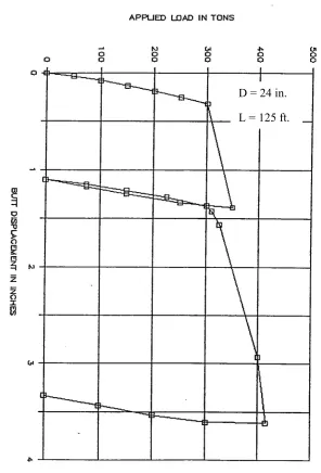
Figure 3.4 – Example of a Load versus Displacement Graph (After LAW Engineering, 1991)
The load versus displacement graph serves two main purposes. First, this graph
can be used to determine when the drilled shaft failed based on a plunging failure
condition in the load test. In Figure 3.4, the shaft displaces in a relatively linear manner
as the loads are applied up to 300 tons. When the 350 ton load increment was applied,
the overall displacement of the shaft approximately tripled to a displacement of
approximately 1.4 inches. This indicated to the operator of the load test that the shaft was D = 24 in.
nearing failure or had failed. At this point, an unload cycle was applied to determine the
permanent shaft displacement and if there was any residual shear strength loss.
Following the unload cycle, the shaft was reloaded past the initial failure point to 400
tons, at which time the shaft plunged 3.6 inches, indicating complete failure.
Second, the load versus displacement graph can be used to determine allowable
shaft loading based on a maximum shaft head deflection. For example, based on the data
shown in Figure 3.4, if the test shaft was built like the planned production shafts and the
maximum allowable shaft head deflection as specified by the structural engineer was 0.25
inches, the maximum allowable load would be 250 tons.
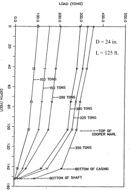
The load versus depth graph serves a related purpose. Figure 3.5 shows a set of
load versus depth curves from the same test shaft as the load versus displacement graph
in Figure 3.4. Load versus depth graphs are used to determine the unit resistance
properties from the load test. As mentioned previously, the maximum allowable load is
determined based on the maximum allowable deflection. Based on the maximum
allowable load, the corresponding curve is selected from the load versus depth graph.
Based on this curve, the load transfer can be determined for each section of the shaft,
with a shaft section being the part of the shaft between two strain gauges. The locations
of the strain gauges are indicated by the points shown on each curve. For example, using
the 350 ton curve in Figure 3.5, the unit skin resistance at the failure load in each segment
Figure 3.5 – Example of a Load versus Depth Graph (After LAW Engineering, 1991)
The section between the top of the Cooper Marl and the bottom of the casing is
approximately 40 feet long. To determine the load carried in this section, the load at the
top of Cooper Marl is subtracted from the load at the bottom of the casing. In this case,
the load at the top of the Cooper Marl is approximately 290 tons and the load at the
bottom of the casing is 210 tons, showing that the load carried in that segment is 80 tons
total. The unit skin resistance can be found from the following equation:
fs= Q
A (3-1)
D = 24 in.
where fs is the unit skin resistance, Q is the total load, and A is the shaft segment surface
area.
In the load test report (LAW Engineering, 1991), the shaft is stated to be 24
inches in diameter. Over a 40 foot section, this equates to a segment surface area of
approximately 250 square feet, thus, an average skin friction of 0.32 tons per square feet
is found from Equation 3-1.
3.8.2 - Osterberg Cell Load Test Data
Load test data from O-Cell load tests is collected for each segment of the test
shaft, as the shaft is split into segments between the Osterberg cells, instead of the shaft
as a whole. The strain and displacement data from each segment is combined to
determine the equivalent behavior to a shaft that is loaded from the top.
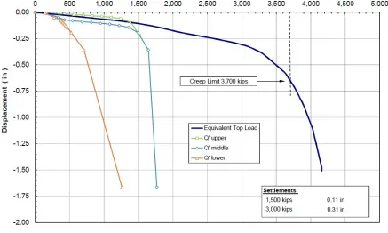
Figure 3.6 is an example of a load versus displacement graph from a two-cell
Osterberg test. Load versus displacement curves for each of the three test shaft segments
are noted as the Q’ upper, Q’ middle, and Q’ lower. Since the segments moved in
different directions (when the top segment moved up, the bottom segment moved down),
the displacement is normalized to the same direction. Then, the three segment curves are
combined to form the equivalent top load curve, which is the curve on the far right of
Figure 3.6. This curve is interpreted in the same manner as the static load test load versus
displacement graph presented in Figure 3.4.
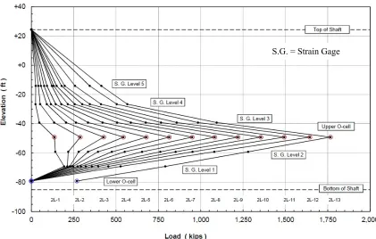
To evaluate the unit skin resistance, the same methodology discussed in Section
3.8.1 is used. One factor to take into account is that for a multi-cell O-Cell load test,
there will be a graph of load versus depth for each load stage, as both cells are generally
not pressurized simultaneously.
Figure 3.7 – Example of an Osterberg Load Test Load versus Depth Graph (After Loadtest, 2014)