An Extremely Efficient Boundary Element Method for Wave Interaction with Long Cylindrical Structures Based on Free-Surface Green’s Function

Article

An Extremely Efficient Boundary Element Method

for Wave Interaction with Long Cylindrical

Structures Based on Free-Surface Green’s Function

Yingyi Liu 1,_{*, Ying Gou} 2 _{and Bin Teng} 2

1 _{Research Institute for Applied Mechanics, Kyushu University, Kasuga, Fukuoka 8168580, Japan}

2 _{State Key Laboratory of Coastal and Offshore Engineering, Dalian University of Technology, Dalian}

116024, China; [email protected] (Y.G.); [email protected] (B.T.) * Correspondence: [email protected]; Tel.: +81-80-8565-7934

Abstract: The present study aims to develop an efficient numerical method for computing the

diffraction and radiation of water waves with horizontal long cylindrical structures, such as floating breakwaters in the coastal region, etc. A higher-order scheme is used to discretize geometry of the structure as well as the physical wave potentials. As the kernel of this method, Wehausen’s free-surface Green function is calculated by a newly-developed Gauss-Kronrod adaptive quadrature algorithm after elimination of its Cauchy-type singularities. To improve its computation efficiency, an analytical solution is derived for a fast evaluation of the Green function that needs to be implemented for thousands of times. In addition, the OpenMP parallelization technique is applied to the formation of the influence coefficient matrix, significantly reducing the running CPU time. Computations are performed on wave exciting forces and hydrodynamic coefficients for the long cylindrical structures, either floating or submerged. Comparison with other numerical and analytical methods demonstrates a good performance of the present method.

Keywords: long cylindrical structure; free-surface Green function; higher-order boundary element

method; multipole expansion; singularity elimination; Gauss-Kronrod; numerical quadrature; OpenMP parallelization

1. Introduction

advantages facilitate the numerical investigation for hydrodynamic performances of such cylindrical structures.

These horizontal cylindrical structures are so long in its axis direction that the problem to be solved could be considered in two-dimensional. In comparison to the three-dimensional wave-structure interaction model within the framework of linear potential flow theory, the present simplified two-dimensional model have much less unknowns on the body surface, since the surface integrations have been substituted by line integrations. In our HOBEM (higher-order boundary element method) model, for a typical frequency domain problem, about 10~50 elements (or in other word less than 100 nodes) are sufficient to represent an arbitrary cross-sectional shape. Therefore, generally about 102_~104 _{evaluations of the Green function are needed for each incident wave period,}

in comparison to those O(106_{) evaluations in the three-dimensional cases (see [12]). Furthermore, by}

taking advantage of the contemporary computational technologies, some special technique may be applied to parallelize the algorithm on multi-processor machines.

Apart from the HOBEM discretization, efficient evaluation of the free-surface Green function is another important issue in this work. Numerous studies have been performed in the field since 1980s. Noblesse and Newman have made the most important contributions for this issue [12-17]. They developed several popular methods, e.g., separating the local component from the far-field one and then calculate them by tabulation algorithm, or making the singular functions slow-varying by subtracting some component and then approximate the resulting functions by Chebyshev approximation. These methods have been simplified in the present model since the problem to be considered is two-dimensional and in infinite water depth, in which an extremely convenient analytical solution can be found for the kernel function. The numerical results in section 3 show the validity and efficiency of the present method.

2. Mathematical Theory and Algorithms

2.1. Governing Equation and Boundary Conditions

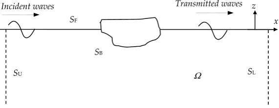
The problem is to consider interactions between linear water waves and a long prismatic rigid structure in arbitrary cross-sectional shape, either floating or submerged in water of infinite depth, as shown in Figure 1. The right-handed Cartesian coordinate system (x, z) is defined, with its origin located at the undisturbed free surface level and the z-axis taken vertically upward. The fluid domain is denoted by Ω, whose boundaries S consists of a free surface boundary SF, an up-side open

boundary SU, a lee-side open boundary SL, and a wetted surface boundary SB on the structure.

Figure 1. Computation domain of the problem.

The fluid is assumed to be inviscid and incompressible, and the motion is assumed irrotational. For the linear small amplitude wave harmonic in time with an angular frequency ω, the velocity potential can be expressed by

(

)

(

)

, , Re _f , , -w

F =

é

_ë

ù

_û

x z t x z t e , (1)

Incident waves Transmitted waves

x z

SU

SB SF

SL

where φ is a time-independent complex velocity potential, which can be further decomposed into 3

0 4

1 i _{j j}

j

f f f w c f

=

= + -

å

where the three components denote incident potential, diffraction potential, and radiation potential, respectively; χj represents displacement of the body motion in each mode (sway, heave or roll), and

φj stands for the corresponding radiation potential to each motion mode.

The incoming wave of amplitude A and frequency ω, propagating in the positive x direction in the water of infinite water depth, can be described by the following incident velocity potential

i 0

igA Kz Kx

e f

w +

= - , (3)

where K is the infinite depth wave number defined by = ⁄ . The four induced wave potentials φj (j =1~4) must satisfy the Laplace equation

2 0

j

f

 = , (4)

and be subjected to various boundary conditions in the fluid domain, including the free surface condition on SF

0

j

j

K z

f f

¶

- =

¶ , (5)

the bottom boundary condition as z→∞

0

j

f

  , (6)

the boundary condition on the surface SB of the structure

(

)

(

)

0

, 4

n n

, 1, 2, 3

j

j

j

n j

f

f ¶

¶ - =

= ¶

¶

=

ìïï

ïí

ïï

ïî

, (7)

and the radiation condition in the far field boundaries SU and SL

lim j i _j 0

x

K x f

f ¥

¶

 =

¶

æ

_ö÷

ç

_÷

ç

_÷

ç

_÷

çè

ø

where n is the normal direction of the body geometry, with its three components n1= nx, n2= nz, n3

=(z-zc)nx-(x-xc)nz, where nx and nz are the x and z components of the unit inward normal, respectively, and

(xc, zc) is the rotation centre. The subscripts j =1, 2, 3 denote the direction of sway, heave and roll for

radiation, respectively, and j =4 stands for diffraction.

2.2. Numerical Techniques

According to Green’s second theorem, by employing Wehausen’s free-surface Green function as the kernel, a boundary integral equation can be obtained as

( )

(

)

( )

(

)

( )

0 0

;

;

n n

f

af = ¶ f - ¶

¶ ¶

é

ù

ê

ú

ê

ú

ë

û

ò

j j

B S

G

G x dS

x x

x x x x , (9)

(

)

(

)

0 1

; ln 2 cos

z

r e

G x d

r K

m z

m x m

m + ¥

= -

-ò

where path of the contour integral passes below the poles at μ = K; coordinate of the source point is

x0 = (ξ, ζ) ; r is the distance between field point and source point, and r1 is the distance between field

point and the image of source point with respect to the free surface.

On the other aspect, if Rankine Green function were employed as the kernel, the boundary integral equation would be

( )

(

)

( )

(

)

( )

0 0

x x x

x ; x x x;

n n

j

j j

F B U L

S S S S

G G dS f af f + + + ¶ ¶ = -¶ ¶

é

ù

ê

ú

ê

ú

ë

û

ò

where the kernel would be simply expressed by

(

)

G = r. (12)

In this paper, we denote the method based on Eq. (9) and Eq. (10) as FSG_BEM, and the method based on Eq. (11) and Eq. (12) as RKG_BEM. The former is applied as the present numerical method, while the latter one is used as a comparison for computational efficiency.

The 3-node isoparametric element is selected to discrete both the geometry of body surface and the physical variables, the shape functions of which being expressed by

( )

(

)

1

1

1 2

h h = h h- , (13)

( )

2 1

h h = -h , (14)

( )

(

)

3

1

1 2

h h = h h+ , (15)

where η is the local coordinate (−1 ≤ ≤ 1). Therefore, the velocity potential and its normal derivative on the boundary surface can be expressed straightforwardly as

[ ]

( )

1

, _k k, k

k

x z h h x z

=

=

å

é

_ë

ù

_û

( )

f h f

= ¶ ¶ = ¶ ¶

é

ù

é

ù

_ê

æ

_ç

ö

_{÷ ú}

ê

ú

_ê

_ç

_ç

÷

_÷

_ú

ê

ú

è

ø

ë

û

å

ê

_ë

ú

_û

Applying the above discretization and the body surface condition Eqs. (5) ~ (8) leads to the following discrete form of the boundary integral equation of Eq. (9)

( )

(

)

( )

( )

( )

(

)

( )

( )

(

)

(

)

( )

(

)

1 ₁ 1

1 0 1 ₁ 1 1 ₁ ; n

; , 4

n

; , 1, 2, 3

N

k

j k j

i k N i N j i B B B G

h J d

G J d j

G n J d j

af h f h h

where NB represents the number of total elements along the body surface, and J(η) the Jacobi matrix

for local-global coordinate transformation, the determinant value of which is calculated by

( )

2 2

dx dz

J

d d

h

h h

=

æ ö

ç

_ç

_ç

÷

_÷

_÷

æ ö

ç

_ç

_ç

÷

_÷

_÷

è ø

è ø

By employing a collocation process for Eq. (18) that the source point is arranged to be put on each grid node on the immersed body surface mesh, a linear algebraic system could be obtained in closed form

[ ]

[ ]

é ù

ë û

where N is the total number of nodes. Solution of the above linear system is sensitive to the diagonal terms of the left-hand side influence matrix [A], which therefore needs to be evaluated precisely with caution. However, direct calculation of these diagonal terms is usually inaccurate and troublesome, due to the high singularity of the Green function in the case when the field point and the source point coincides with each other. Fortunately, this weakness can be avoided by considering a constant flux across the fluid (φ =1), thereafter we obtain

(

)

1 ,

, 1, ...,

N

ii ij

j j i

A A i N

= ¹

= -

å

In calculation of each influence coefficient Aij (j ≠ i), OpenMP parallelization technique is employed

to distribute the computation burden on multiple processors of a single computer. The parallelization works well since calculation of the influence coefficient on one element is independent from that on another element. After that, the Gauss elimination algorithm is used to solve the linear system, which is extremely robust regardless of arbitrary shape of the structure.

Given solution for the linear system, we can get the wave exciting force, added mass and added damping by directly integrating the corresponding hydrodynamic pressure over the immersed body surface, respectively, i.e. ,

(

)

B

j j

S

f = rw

ò

and

i

S

B

ij

ij i j

S

b

a r fn d

w

+ =

ò

2.3. Direct Calculation of Free-surface Green’s Function

As pointed out in the previous section Introduction, accurate calculation of the free-surface Green function is of great importance to the final solution of the problem. At a preliminary step, we may apply the function decomposition method which was proposed by Newman [17]. In terms of the following two coordinates

(

)

X=K x-x Y=K z+z

(

)

1 1

ln r 2 , 2 i Ycos

G F X Y e X

r

p

-= - - , (23)

where i denotes the imaginary unit. The singular part of Eq. (23) is

(

)

1 , P.V. ₀ cos

1

kY

e

F X Y kXdk

k

-¥

=

-ò

where P.V. denotes Cauchy principle value of the integral. The principle task here is to evaluate the normalized real function F1(X, Y) for all relevant values of input parameters (X, Y) of possible physical

interest [17]. Using the identity

2

0

P.V. 0

1

dk

k- =

ò

Eq. (24) can be written [18] in a more convenient form from the view point of numerical evaluation

(

)

( )

( )

( )

1 1 1

1 _{0 2}

1 ,

1 1

f k f f k

F X Y dk dk

k k

¥

-= +

-

-ò

ò

where

( )

1 cos

kY

f k =e- kx. (26)

In the neighborhood of k = 1, linear approximation may be applied such that

( )

( )

_{( )}

_[

_]

1 1

1 1

cos sin

1

kY

f k f

f k e Y kx X kx

k

-= = - +

- . (27)

Hence Eq. (25) can be evaluated accurately by an adaptive Gauss-Kronrod-type quadrature algorithm (see Appendix A).

Following a similar procedure, the derivatives of the Green function with respect to x and z can be normalized as

(

)

(

)

2 2

1 1 1

2 , 2 i Ysin

x

G x KF X Y Ke X

r r

x p

-= -

æ

ç

_ç

_ç

ö÷

÷

_÷

÷

çè

ø

(

) (

)

₍

₎

3

2 2

1

2 , 2 i Ycos

z

z z

G KF X Y Ke X

r r

z z

p

-- +

= - - - ， (29)

where their singular parts are

(

)

2 , P.V. ₀ sin

1

kY

ke

F X Y kXdk

k

-¥

=

-ò

(

)

3

0

, P.V. cos

1

kY

ke

F X Y kXdk

k

-¥

=

Eq. (30) and Eq. (31) can be formulated as the same form as Eq. (25), where

( )

2 sin

kY

f k =ke- kx, (32)

( )

3 cos

kY

f k =ke- kx, (33)

( )

[

]

'

-2 = sin - sin cos

kY

f k e kx kY kx+kX kx , (34)

( )

[

]

'

3 cos cos sin

kY

f k =e- kx-kY kx-kX kx . (35)

2.4. Fast Evaluation by analytical method

Although calculation of the free-surface Green function becomes applicable following the method described in Section 4, a large amount of computation time would be consumed due to the direct integration by the meticulous adaptive numerical quadrature method. The reason for that is the effort of dealing with singularity in the denominator, as well as the oscillating inherence of the integrand. A possible way for its improvement is to derive an alternative analytical expression which can automatically remove the troublesome singularity, as described below.

Based on McIver [19], we can obtain the following representation for the principle value of the following singular integral without too much of difficulty

( )

( )

(

₍

₍

₎

₎

)

₍

₎

( )

₍

₍

₎

₎

₍

₎

( )

(

₍

₍

₎

₎

)

₍

₎

i

1 i

0

i

1

i i , 0, 0

P.V. d , 0, 0

i i , 0, 0

K z KX

z X

K z

K z KX

e E K z KX X z

e

e Ei K z X z

K

e E K z KX X z

z

m z m

z

z

p z z

m z z

m

p z z

+ +

+ +

¥ ₊

+ +

ìï _{- + + + < + £}

ïï ïïï

= -_íï - + = + £

- _ïï

ï + + + > + £

ïïî

ò

where the exponential integrals are defined as

(

)

t x

-e

Ei(x) = dt, x > 0 t

∞



(

)

1

-t

Z

e

E (Z) = dt, arg Z <π

t

∞



LetZ = K z +

(

)

{ }

( )

(

)

{

}

(

)

(

)

{

}

(

)

( )

(

)

{

}

(

)

1

1

1

Re i , 0, 0

Re ln 2 Re , 0, 0

Re i , 0, 0

Z

Z

Z

e E Z X z

r

G e Ei Kz X z

r

e E Z X z

p z

z

p z

ìï _{- + < + £}

ïï ïïï

= - _íï - - = + £

ïï

ï + > + £

ïïî

, (39)

while the imaginary part is obtained by applying the residue theorem, after which we find

{ }

( )

Im G = -2i Rep eZ , (40)

( )

d

Z

E Z _e

Z Z

-= - , (41)

( )

d

z

Ei z e

z z

-= , (42)

it is possible to calculate derivatives of the Green function with respect to x and z, in which their real parts are corresponding to

{ } (

)

( )

(

)

(

)

(

)

( )

(

)

(

)

1

2 2

1

1

i

Re i i , 0, 0

1 1

Re 2 0, 0, 0

i

Re i i , 0, 0

Z

x

Z

K

Ke E Z X z

Z

G x X z

r r

K

Ke E Z X z

Z

p z

x z

p z

ì ì ü

ï ï_ï ï_ï

ï _{í - + - ý < + £}

ïï ï ï

ï ïî ïþ

æ ö_{÷ ïï}

ç _÷ ï

= - ç_ççè - ÷_÷÷- í_ï = + £

ø _{ïï ì ü}

ï ï

ï ï _{+ -} ï _{> + £}

ï í ý

ï _{ï ï}

ï ïî ïþ

ïî

, (43)

{ }

(

) (

)

( )

(

)

(

)

(

)

(

)

( )

(

)

(

)

1

2 2

1

1

Re i , 0, 0

1

Re 2 Re , 0, 0

Re i , 0, 0

Z

z z

Z

K

Ke E Z X z

Z

z z

G Ke Ei Kz X z

KZ

r r

K

Ke E Z X z

Z

p z

z z

z

p z

ì ì ü

ï ï_ï ï_ï

ï _{í - + - ý < + £}

ïï ï ï

ï ïî ïþ

ïï

- + ï_ï ìï_ï üï_ï

= - - í_ï í_ï- - + ý_ï = + £

ï ï

î þ

ïï

ï _{ìï üï}

ï _{ï ï}

ï _{í + - ý > + £}

ï _{ï ï}

ï _{ïî ïþ}

ïî

, (44)

respectively. Their imaginary parts are easily obtained by applying the residue theorem as

{ }

( )

Im 2i Im Z

x

G = Kp e , (45)

{ }

( )

Im G_z = -2iKpRe eZ . (46)

Through this way, we are able to calculate the free-surface Green function in a fast manner, since Eqs. (39) ~ (40) and Eqs. (43) ~ (46) are all in analytical form, which just simply consists of the exponential functions and the trigonometric functions.

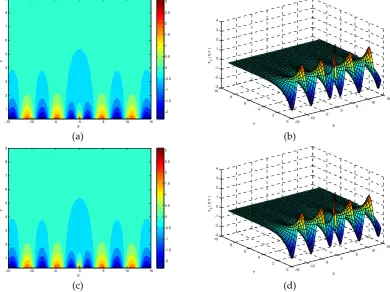
A comparison between plots of the three singular functions F1(X, Y), F2(X, Y) and F3(X, Y) by the

direct integration method and the analytical solution method is shown in Figures 2~4. In general, the two methods get almost same results which are hard to be distinguished from each other. It is obviously to see that F1(X, Y) and F3(X, Y) are even functions in symmetric with respect to the Y axis,

while F2(X, Y) is an odd function which is anti-symmetric about the Y axis. Remarkable variations

(a) (b)

(c) (d)

Figure 2. Comparison of the singular function F1(X, Y) calculated by the two methods: (a) Contour plot by direct integration; (b) Oblique view by direct integration; (c) Contour plot by analytical solution; (d) Oblique view by analytical solution.

(a) (b)

(c) (d)

X

Y

-15 -10 -5 0 5 10 15

1 2 3 4 5 6 7 8 9 -2 -1.5 -1 -0.5 0 0.5 1 1.5 -15 -10 -5 0 5 10 15 0 2 4 6 8 10 -3 -2 -1 0 1 2 3 X Y F1 ( X,Y ) X Y

-15 -10 -5 0 5 10 15

1 2 3 4 5 6 7 8 9 -2 -1.5 -1 -0.5 0 0.5 1 1.5 -15 -10 -5 0 5 10 15 0 2 4 6 8 10-3 -2 -1 0 1 2 3 X Y F1 ( X,Y ) X Y

-15 -10 -5 0 5 10 15

1 2 3 4 5 6 7 8 9 -2 -1.5 -1 -0.5 0 0.5 1 1.5 2 -15 -10 -5 0 5 10 15 0 2 4 6 8 10-3 -2 -1 0 1 2 3 X Y F2 ( X,Y ) X Y

-15 -10 -5 0 5 10 15

Figure 3. Comparison of the singular function F2(X, Y) calculated by the two methods: (a) Contour plot by direct integration; (b) Oblique view by direct integration; (c) Contour plot by analytical solution; (d) Oblique view by analytical solution.

(a) (b)

(c) (d)

Figure 4. Comparison of the singular function F3(X, Y) calculated by the two methods: (a) Contour plot by direct integration; (b) Oblique view by direct integration; (c) Contour plot by analytical solution; (d) Oblique view by analytical solution.

3. Numerical Results and Discussion

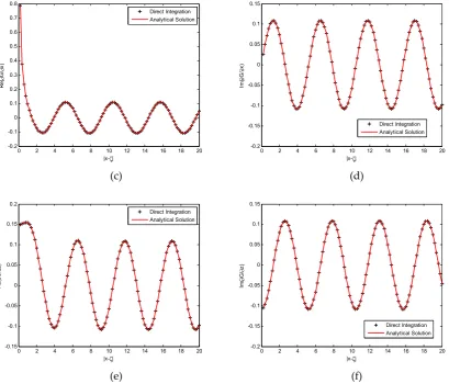
Based on the direct calculation method and the analytical solution method described above, values of the free-surface Green function and its derivatives are compared, as shown in Figures 5 ~ 6, against variation of the physical horizontal distance |x-ξ| between the source and the field points. Both the real part and the imaginary part are compared, showing that they coincide fairly well with each other. It should be noted that calculation of the imaginary parts is relatively straightforward since the real parts contain troublesome principal values of the singular integrals.

(a) (b)

X

Y

-15 -10 -5 0 5 10 15

1 2 3 4 5 6 7 8 9

-2 -1.5 -1 -0.5 0 0.5 1 1.5 2 2.5 3

-15 -10 -5 0

5 10 15

0 2 4 6 8 10-3

-2 -1 0 1 2 3 4

X Y

F3

( X

,Y

)

X

Y

-15 -10 -5 0 5 10 15

1 2 3 4 5 6 7 8 9

-2 -1.5 -1 -0.5 0 0.5 1 1.5 2 2.5 3

-15 -10 -5 0

5 10 15

0 2 4 6 8 10-3

-2 -1 0 1 2 3 4

X Y

F3

(

X,Y )

0 2 4 6 8 10 12 14 16 18 20

-0.2 -0.15 -0.1 -0.05 0 0.05 0.1 0.15

|x-ζ|

Re

(G

)

Direct Integration Analytical Solution

0 2 4 6 8 10 12 14 16 18 20

-0.1 -0.05 0 0.05 0.1 0.15

|x-ζ|

Im

(G

)

(c) (d)

(e) (f)

Figure 5. Comparison of two methods for calculating Wehausen’s Green function and its derivatives (K = 1.2 m-1_, ζ _{= -1.0m, z = -1.0m): (a) Real part value of G; (b) Imaginary part value of G; (c) Real part} value of Gx; (d) Imaginary part value of Gx; (e) Real part value of Gz; (f) Imaginary part value of Gz.

(a) (b)

0 2 4 6 8 10 12 14 16 18 20

-0.2 -0.1 0 0.1 0.2 0.3 0.4 0.5 0.6 0.7 0.8

|x-ζ|

Re

(∂ G/∂

x)

Direct Integration Analytical Solution

0 2 4 6 8 10 12 14 16 18 20

-0.2 -0.15 -0.1 -0.05 0 0.05 0.1 0.15

|x-ζ|

Im

(∂ G/∂

x)

Direct Integration Analytical Solution

0 2 4 6 8 10 12 14 16 18 20

-0.15 -0.1 -0.05 0 0.05 0.1 0.15 0.2

|x-ζ|

Re

(∂ G/∂

z)

Direct Integration Analytical Solution

0 2 4 6 8 10 12 14 16 18 20

-0.2 -0.15 -0.1 -0.05 0 0.05 0.1 0.15

|x-ζ|

Im

(∂ G/∂

z)

Direct Integration Analytical Solution

0 2 4 6 8 10 12 14 16 18 20

-2.5 -2 -1.5 -1

|x-ζ|

Re

(G

)

Direct Integration Analytical Solution

0 2 4 6 8 10 12 14 16 18 20

-0.9997 -0.9997 -0.9997 -0.9996 -0.9996 -0.9996 -0.9996 -0.9996 -0.9995 -0.9995

|x-ζ|

Im

(G

)

(c) (d)

(e) (f)

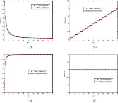
Figure 6. Comparison of two methods for calculating Wehausen’s Green function and its derivatives (K = 0.001 m-1_, ζ _{= -0.1m, z = -0.2m): (a) Real part value of G; (b) Imaginary part value of G; (c) Real} part value of Gx; (d) Imaginary part value of Gx; (e) Real part value of Gz; (f) Imaginary part value of

Gz.

Due to different nature of the free-surface Green function when the source point locates at the free surface or not, we need to verify the results for both floating bodies and submerged bodies. In order to compare with some existing analytical results, we select horizontal floating/submerged circular cylinders for the benchmark examples. When the cylinder is submerged, its wet body surface should be considered as a completely immersed circle; when it is floating with its centroid locates on exactly the mean water surface, whereas its wet body surface should be treated as a half circle. Their analytical solutions are all obtained based on the so-called multipole expansion method, which were published in [2,20] for submerged circle in water of infinite depth, and in [1,21] for half circle in water of infinite depth. The RKG_BEM is also implemented for comparison, in which all the boundaries should be taken into consideration; whereas for the FSG_BEM, only the body surface needs to be meshed. In the following illustration, LF, LU, LL and LB denote the length of the boundaries as shown

in Figure 1, respectively, and NF, NU, NL and NB denote the number of elements meshed on the

boundaries, respectively.

Table 1. Mesh specifications for the case shown in Figure 4

Method LF LU LL LB NF NU NL NB

FSG_BEM / / / π a / / / 10

RKG_BEM 60a 20a 20a π a 240 90 90 30

0 2 4 6 8 10 12 14 16 18 20

0 0.1 0.2 0.3 0.4 0.5 0.6 0.7 0.8 0.9

|x-ζ|

Re

(∂ G/∂

x)

Direct Integration Analytical Solution

0 2 4 6 8 10 12 14 16 18 20

0 0.5 1 1.5 2 2.5x 10

-5

|x-ζ|

Im

(∂ G/∂

x)

Direct Integration Analytical Solution

0 2 4 6 8 10 12 14 16 18 20

-0.8 -0.7 -0.6 -0.5 -0.4 -0.3 -0.2 -0.1 0

|x-ζ|

Re

(∂ G/∂

z) Direct Integration

Analytical Solution

0 2 4 6 8 10 12 14 16 18 20

-1.5 -1 -0.5 0 0.5 1

|x-ζ|

Im

(∂ G/∂

z)

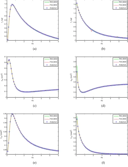
Figure 7 shows modules of complex exciting force, added mass and added damping of a semi-immersed cylinder of radius a in comparison with those computed by the RKG_BEM and the analytical multipole expansion method [20].The corresponding meshes used by the two boundary element methods are specified in Table 1. In Figure 7, the present method based on the analytically evaluated free-surface Green function achieves good agreement with both of the other two methods. Noted that, there are some odd points on the curve calculated by the FSG_BEM. This phenomenon should be attributed to the so-called “irregular frequencies” [22], since the discrete boundary integral equation is ill-conditioned to be uniquely solvable at these frequencies.

(a) (b)

(c) (d)

(e) (f)

Figure 7. Comparison of hydrodynamic characteristics of a floating cylinder, in semi-immersed circle of radius a: (a) Sway exciting force; (b) Heave exciting force; (c) Sway added mass; (d) Heave added mass; (e) Sway added damping; (f) Heave added damping.

0 1 2 3 4 5 6

0.4 0.5 0.6 0.7 0.8 0.9 1 1.1 1.2 1.3

Ka

fx

/(ρ

g)

RKG_-BEM FSG_-BEM Analytical

0 1 2 3 4 5 6

0 0.2 0.4 0.6 0.8 1 1.2 1.4 1.6 1.8

Ka

fz

/(ρ

g)

RKG_-BEM FSG_-BEM Analytical

0 1 2 3 4 5 6

0 0.1 0.2 0.3 0.4 0.5 0.6 0.7

Ka

a22 /(ρπ

a

2)

RKG_-BEM FSG_-BEM Analytical

0 1 2 3 4 5 6

0.2 0.3 0.4 0.5 0.6 0.7 0.8 0.9 1

Ka

a33

/(

ρπ

a

2)

RKG_-BEM FSG_-BEM Analytical

0 1 2 3 4 5 6

0 0.05 0.1 0.15 0.2 0.25 0.3 0.35 0.4 0.45

Ka

b22 /(ρπ

ω

a

2)

RKG_-BEM FSG_-BEM Analytical

0 1 2 3 4 5 6

0 0.1 0.2 0.3 0.4 0.5 0.6 0.7 0.8 0.9 1

Ka

b33

/(

ρπ

ω

a

2)

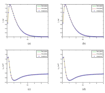
Figure 8 shows modules of complex exciting forces, added mass and added damping of a submerged cylinder in comparison with those computed by RKG_BEM and analytical multipole expansion method [21]. In the solution of multipole expansion method, we derive a new exact formulation (see Appendix B) for the multipole expansion coefficient Amn which is troublesome for

calculation due to its high singularity in the integrand. In this case, the radius of the cylinder is a, and the submergence of its centroid is f/a=1.5. The meshes used by the two boundary element methods are specified in Table 2. In Figure 8, similar to the case of semi-circle, the present method based on the analytically evaluated free-surface Green function highly agrees with both of the other two methods. In addition, there is no ‘irregular frequencies’ phenomenon, which proves the knowledge that for submerged bodies, the solution is always unique.

Table 2. Mesh specifications for the case shown in Figure 5

Method LF LU LL LB NF NU NL NB

FSG_BEM / / / 2π a / / / 10

RKG_BEM 60a 20a 20a 2π a 240 90 90 60

(a) (b)

(c) (d)

0 1 2 3 4 5 6

0 0.2 0.4 0.6 0.8 1 1.2 1.4 1.6

Ka

fx

/(ρ

g)

RKG_-BEM FSG_-BEM Analytical

0 1 2 3 4 5 6

0 0.2 0.4 0.6 0.8 1 1.2 1.4 1.6

Ka

fz

/(

ρ

g)

RKG_-BEM FSG_-BEM Analytical

0 1 2 3 4 5 6

0.4 0.6 0.8 1 1.2 1.4 1.6 1.8

Ka

a22 /(ρπ

a

2)

RKG_-BEM FSG_-BEM Analytical

0 1 2 3 4 5 6

0.4 0.6 0.8 1 1.2 1.4 1.6 1.8

Ka

a33

/(

ρπ

a

2)

(e) (f)

Figure 8. Comparison of hydrodynamic characteristics of a submerged cylinder: (a) Sway exciting force; (b) Heave exciting force; (c) Sway added mass; (d) Heave added mass; (e) Sway added damping; (f) Heave added damping.

(a) (b)

Figure 9. CPU time of the two boundary element methods based on different calculation schemes of the free-surface Green function in sequential or parallel mode: (a) Comparison for the direct integration method; (b) Comparison for the analytical solution method.

Figure 9 shows a comparison of computation time (unit: sec) for 60 incident wave periods between the BEMs (boundary element methods) based on the direct integration and the analytical solution of the free-surface Green function, in either sequential mode or parallel mode. The computations are implemented on a SONY laptop, with an Intel(R) Core(TM) i7-2670QM CPU of 2.2 GHz, on 64-bit Windows operating system. The OpenMP parallelization technique have been applied in the parallel mode. In Figure 9, a remarkable trend of reduction in CPU time is shown by using the parallel mode, which tends to be more apparent with increasing number of the total elements, in both Figure 9(a) and Figure 9(b). On the other hand, the analytical-based Green function has saved a lot of computation time for the BEM analysis. Roughly speaking, it has improved the computation speed for around 27~36 times in the sequential mode, and 12~60 times in the parallel mode, in comparison to the direct-integration Green function method, depending on the number of total elements in the input mesh of geometry.

0 1 2 3 4 5 6

-0.1 0 0.1 0.2 0.3 0.4 0.5 0.6 0.7 0.8

Ka

b22 /(ρπ

ω

a

2)

RKG_-BEM FSG_-BEM Analytical

0 1 2 3 4 5 6

-0.1 0 0.1 0.2 0.3 0.4 0.5 0.6 0.7 0.8

Ka

b33 /(ρπ

ω

a

2)

RKG_-BEM FSG_-BEM Analytical

0 20 40 60 80 100 120

0 100 200 300 400 500 600

Number of total elements

CP

U t

im

e

(s

)

DrG_-BEM_-sequential DrG_-BEM_-parallel

0 20 40 60 80 100 120

0 2 4 6 8 10 12 14

Number of total elements

CP

U t

im

e

(s

)

(a) (b)

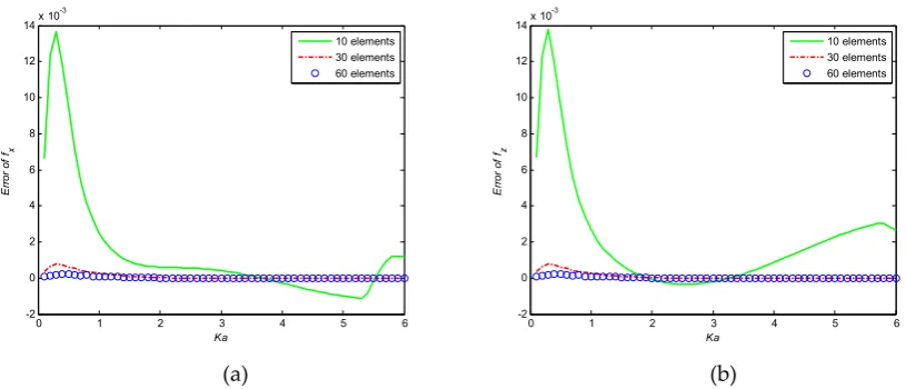
Figure 10. Convergence test of the present method with respect to the number of elements: (a) Sway exciting force; (b) Heave exciting force.

Figure 10 shows convergence rate of the present FSG_BEM using analytical solution Green function with respect to the number of boundary elements. No evident difference can be observed in accompany with the increase of the number of elements from 10 to 40. This may suggest that, for such a cylinder, only a few elements are sufficient to obtain a high accuracy, which demonstrates a perfect convergence of the present boundary method by utilizing the analytically evaluated free-surface Green function.

4. Conclusions

In this paper, we presented a FSG_BEM, which applies a 3-node higher-order scheme, and an analytical algorithm of the free-surface Green function. Various numerical results show that the present method deserves high accuracy, good convergence, and fast computation efficiency.

Acknowledgments: The authors gratefully acknowledge the financial support provided by National Natural Science Foundation of China (Grant Nos. 11072052, 51221961), and the financial support provided by the National Basic Research Program of China (973-Program) (Grant No. 2011CB013703). The authors gratefully appreciate Prof. Phil McIver of Loughborough University, and Dr. R. Porter of Bristol University, for their most valuable suggestions on the issue of removing the singularity.

Author Contributions: Yingyi Liu developed the algorithm of free-surface Green function, performed all the calculations in the paper and wrote the manuscript. Ying Gou did proofreading and polished the English. The HOBEM code was programmed by professor Bin Teng, who also was the supervisor of this work during the study of Yingyi Liu in DUT.

Conflicts of Interest: The authors declare no conflict of interest

Abbreviations

RKG_BEM: Rankine Green function based Boundary Element Method

FSG_BEM: Free-surface Green function based Boundary Element Method

DrG_BEM: Boundary Element Method based on direct integration of the free-surface Green function

AlG_BEM: Boundary Element Method based on analytical solution of the free-surface Green function

Appendix A

Let [a, b] be the integration interval, f be a Riemann integrable function, the following target integral

0 1 2 3 4 5 6

-2 0 2 4 6 8 10 12 14x 10

-3

Ka

Er

ro

r o

f fx

10 elements 30 elements 60 elements

0 1 2 3 4 5 6

-2 0 2 4 6 8 10 12 14x 10

-3

Ka

Er

ro

r o

f fz

( )

b

a

I=

ò

can be approximated by adding n+1 Kronrod points to the n-point Gauss quadrature rule, so that the function values produced by the lower-order rule can be re-used. This formula is called as Kronrod extension of Gaussian rules [23], which has a maximum degree of exactness 3n+1, i.e.,

( )

( )

* *

3 1

1 1

,

n n

i i k k n

i k

I w f x w f x f P

+

+

= =

=

å

å

where xi are the Gauss nodes and ωi the corresponding weights, ∗and ∗denote the Kronrod nodes

and corresponding weights, respectively.

The difference between a Gauss quadrature rule and its Kronrod extension are often used as an estimate of the approximation error suggested by Piessens et al. [24]:

[ ]

[ ]

(

)

2 1

200 G a b_n , K _n a b,

e= - ₊ , (A3)

where Gn represents the approximation of the initial Gaussian rule, and K2n+1 the approximation of its

Kronrod extension.

Using the Gauss-Kronrod rule, an adaptive integral algorithm can be developed [25]:

Step 1. Firstly, use n-point Gauss rule and 2n+1-point Gauss-Kronrod rule to integrate f(x) on the interval [a, b], respectively. Two approximations of the integral, i.e., Gn and K2n+1, will be obtained, as

well as Eq. (A3). If the error estimation is smaller than a prescribed tolerance Eps, the more accurate approximation K2n+1 is accepted as the final integral value; else, go to Step 2.

Step 2. Divide interval [a, b] into two equal parts, i.e., [a, m] and [m, b], where m = (a + b)/2, and compute the two sub-integrals independently

( )

( )

m b

a m

I=

ò

ò

Again, the two respective approximations and , as well as the local error estimate εi _{will be}

attained

[ ]

[ ]

(

)

2 1

200 , ,

i i i

n n

G a b K a b

e = - ₊ , (A5)

where the superscript denotes the ith sub-interval. If εi _{is smaller than Eps, accept as the final}

integral value on ith interval, and stop the circulation; if not, continue to subdivide the sub-intervals and repeat Step 2.

Appendix B

In the multipole expansion method, Linton and McIver [20] gives an expression for wave scattering potential of a submerged horizontal cylinder in series form

1

1

n n n n

a

f a f

¥ +

=

=

å

where

i

i

0

n

m m

n n mn

m

e

A r e r

q

q f

- ¥

-=

= +

å

( )

(

)

1 2 0

1

! 1 !

m n

m n mn

K

A e d

m n K

mz

m

m m

m +

¥

+

-- +

=

where a is the radius and ζ the submergence. Calculation of the multipole expansion coefficients Amn

is not a trivial task, since usually a direct integration method will be adopted which will leads to some substantial numerical errors. By the Newton’s binomial theorem and through integration by parts, we derive the following series representations for its accurate calculation:

( )

( )

Re i Im

mn mn mn

A = A + A , (B4)

where

( )

( )

(

)

(

)

(

)

(

_{) ( )}

(

)

(

)

₍

₎

2

2

3 2

2 2 1 1

0 1

1 1

Re 1 ! 2

! 1 ! 2

1 ! 2 1

1 2

1 ! ₂ ! 2

m n m n

K

mn

j i K

m n m n i

m n K m n

m n i

i j

A m n Ke

m n

m n K e K m n

K e K Ei K

m n i i j

z

z

z

z

z

z z

z

+ +

-+ - +

-+ - - + +

-= =

-= - + - + ⋅

-+ - +

-+ - -

-+ - -

-ìïæ ö

ïç ÷_÷

íç_{ç ÷}

ïè ø

ïî

é æ_ç ö_{÷ ùüïï}

ê ç_ç ÷_÷ ú_ý

ê _ççè ÷_÷ø ú_ï

ê úï

ë

å

å

, (B5)

and

( )

( )

(

)

1

Im 2

! 1 !

m n

m n K mn

A K e

m n

z

p +

+

-=

- , (B6)

where m³0,n³1, ,m n ZÎ *.

References

1. Ursell, F. On the heaving motion of a circular cylinder on the surface of a fluid. Q. J. Mech. Appl. Math. 1949, 2, 218-231.

2. Ursell, F. Surface waves on deep water in the presence of a submerged circular cylinder I. P. Camb. Philos. Soc. 1950, 46,141-158.

3. Evans, D. V.; Linton, C. M. Active devices for the reduction in wave intensity. Appl. Ocean Res. 1989, 11, 26– 32.

4. Bai, K. J. Diffraction of oblique waves by an infinite cylinder. J. Fluid Mech. 1975, 68, 513–535. 5. Garrison, C. J. Interaction of oblique waves with an infinite cylinder. Appl. Ocean Res. 1984, 6, 4-15. 6. Politis, C. G.; Papalexandris, M. V.; Athanassoulis, G. A. A boundary integral equation method for oblique

water-wave scattering by cylinders governed by the modified Helmholtz equation. Appl. Ocean Res. 1984, 24, 215–233.

7. Zheng, Y. H.; Shen, Y. M.; Ng, C. O. Effective boundary element method for the interaction of oblique waves with long prismatic structures in water of finite depth. Ocean Eng. 2008, 35, 494-502.

8. Dean, R.G.; Ursell, F. Interaction of a fixed, semi-immersed circular cylinder with a train of surface waves. Technical Report. No.37, Hydrodynamic Lab, MIT, USA, 1959.

9. Martin, P.A.; Dixon A.G. The scattering of regular surface waves by a fixed, half-immersed, circular cylinder. Appl. Ocean Res. 1983, 5, 13-23.

10. Wehausen, J.V.; Laitone, E.V. Surface waves. In Encyclopedia of Physics; Springer Verlag: Berlin, German, 1964; Volume 9, pp. 446-778.

11. Haskind, M.D. The diffraction of waves about a moving cylindrical vessel. Prikl. Mat. Mikh. 1953, 17,431-442.

12. Newman, J. N. The approximation of free-surface Green functions. In Wave Asymptotics; Martin, P. A., Wickham G. R., Eds.; Cambridge University Press: Cambridge, England, 1992; pp. 107-135.

14. Telste, J.G.; Noblesse, F. Numerical evaluation of the Green Function of water-wave radiation and diffraction. J. Ship Res. 1986, 30, 69-84.

15. Ponizy B.; Noblesse, F.; Ba, M.; Guilbaud, M. Numerical evaluation of free-surface Green functions. J. Ship Res. 1994, 38, 193–202.

16. Newman, J. N. An expansion of the oscillatory source potential. Appl. Ocean Res. 1984, 6, 116-117. 17. Newman, J. N. Algorithms for free-surface green’s function. J. Eng. Math. 1985, 19, 57–67.

18. Monacella, V. J. The distribution due to a slender ship oscillating in a fluid of finite depth. J. Ship Res. 1966, 10, 242–252.

19. McIver, M. An example of non-uniqueness in the two-dimensional linear water wave problem. J. Fluid Mech. 1996, 315, 257-266.

20. Linton, C. M.; McIver, P. Handbook of mathematical techniques for wave/structure interactions. CRC Press: London, England, 2001.

21. Yan, B.; Bai, W.; Liu, Y.Y.; Gou, Y.; Ning, D.Z. An analytical investigation on floating cylindrical breakwaters with different constraints. Ocean Eng. (under review)

22. Martin, P. A. On the null-field equations for water-wave radiation problems. J. Fluid Mech. 1981, 113, 315-332.

23. Kronrod, A. S. Nodes and weights of quadrature formulas-sixteen-place tables (Authorized translation from the Russian). Consultants Bureau: New York, USA, 1965.

24. Piessens, R.; Doncker-Kapenga, E. De; Uberhuber, C. W.; Kahaner, D. K. QUADPACK-a subroutine package for automatic integration. Springer-Verlag: Berlin, German, 1983.

25. Gander, W.; Gautschi, W. Adaptive quadrature-revisited. Technical Report 306, Department of Computer Science, ETH Zurich, Switzerland, 1998.