A Set of Simple Numerical Pattern Synthesis Algorithms for Anti-Jamming with Superdirective Receiving Array

(1)

A Set of Simple Numerical Pattern Synthesis Algorithms

for Anti-Jamming with Superdirective Receiving Array

Huajun Zhang, Huotao Gao*, Huaqiao Zhao, Ting Cao, and Boya Li

Abstract—Although a superdirective array can acquire maximum directive gain with electrically small array, in some practical applications, low sidelobe and deep nulls are also important, which can effectively inhibit directional interference. In this work, a set of simple superdirective pattern synthesis methods are proposed. By introducing diagonal loading factor and adding virtual jamming constraints, they can keep suitable tradeoff among directive gain, efficiency and anti-jamming performance. Besides, easy realization is another good feature of the proposed methods.

1. INTRODUCTION

Aiming to maximize directive gain and overcome external interference with electrically small arrays, the concept of superdirective pattern synthesis has been proposed [1–4]. It claims the theoretical possibility of arbitrarily high directivity from an array of given aperture or overall length, even if element spacing is suﬃciently compact. Relative algorithms are termed super-gain arrays techniques [5]. Based on the theoretical assumption, sensor array with ultra-small aperture can also acquire the same directive gain or signal-to-noise ratio (SNR) as conventional array with half-wavelength aperture. This is quite attractive in engineering application. Especially in HF band, to achieve high angular resolution and suppress external noise, electrical size of conventional receiving array is tremendous as its working wavelength is 10–100 m. Huge array brings a lot of inconvenience, such as high cost, poor mobility, being vulnerable to attack, etc. Consequently, miniaturization of huge arrays generates considerable interest.

However, classical superdirective arrays have some inherent shortcomings, such as low radiation efficiency and poor robustness. For example, consider a 9-element linear broadside array of copper half-wave dipoles with a overall length of 1/4λ. If the specified directive gain reaches 8.5 times greater than a single dipole, corresponding array efficiency is only 10−14_{, and corresponding jitter}

amplitude of excitation currents must be controlled within 10−11 _{[5], which is technically unrealistic}

at present. Therefore, certain constraint conditions must be imposed to make super-gain array more feasible in practical situations. Newman et al., Zhou et al., etc. have introduced sensitivity constraint in optimization of maximum directive gain. Zhang et al. apply steering vector mismatch to model the uncertainty of a super-gain array. Most of these approaches can be classified as diagonal-loading method [6–10]. Based on these theoretical contributions, superdirective arrays gradually enter engineering application stage. Meanwhile, people find that constrained optimal directivity (CODG) methods still need to be improved. Under given array distribution, such as uniform circular array, their first sidelobe levels remain almost unchanged, which is irrelevant with elements number. This provides array with rather limited anti-jamming effect. After all, ultimate design objective is to reserve signal of interest (SOI) while suppressing or even eliminating external noise and disturbance. Therefore, it will be meaningful to study some optimal algorithms which can realize sidelobe or null control.

Received 20 May 2016, Accepted 24 August 2016, Scheduled 8 September 2016 * Corresponding author: Huotao Gao ([email protected]).

(2)

Refs. [11, 12] adopt the second-order cone programming (SOCP) in reduction of sidelobe levels. But its parameter selection criteria are rather complex, and the method requires array to be accurately calibrated, which is not practical in engineering. Traditional linear constrained optimal directive gain (L-CODG) method can easily form deep nulls at prescribed direction [13–16], but it can hardly satisfy requirements of robustness and efficiency indicators. Here, a set of new pattern synthesis techniques are proposed. The first method forms deep and broaden nulls to suppress high-power interference from centralized direction. The second method uses low sidelobe level to inhibit dispersed interference. By introducing diagonal loading factor, superdirective arrays obtain effective compromise among efficiency, robustness and anti-jamming performance. Besides, the proposed methods are simpler in engineering implementation.

The rest of this paper is arranged as follows. In Section 2, problems and existing solutions are reviewed. Section 3.1 introduces the nulling based method. Section 3.2 analyzes performance of the proposed method by numerical examples. Similarly, Section 4.1 gives the low-sidelobe based method. Relative numerical analysis is shown in Section 4.2. Section 5 draws a ﬁnal conclusion.

2. PROBLEM FORMULATION

In order to facilitate analysis, we assume that an antenna array consists ofM isotropic elements which uniformly distribute at known locations. Applying a set of complex excitation weights w, radiation pattern of the array can be steered towards a predetermined direction (θ0, φ0). For HF superdirective

array, directivityG(θ0, φ0) and eﬃciencyηare key indexes, and they should meet following relationship:

G(θ0, φ0) =

wHNw wH_Rw, η=

wHNw

MwH_w (1)

whereN=a(θ0, φ0)aH(θ0, φ0) and R= ₄1_π

2π 0

_π

0 sinθa(θ, φ)aH(θ, φ)dθdφ. a(θ, φ) is steering vector of

the array, and (·)H denotes Hermitian transpose. Using distortionless constraint wHa(θ0, φ0) = 1 over

signal of interest (SOI) direction, the above formula can be simpliﬁed as:

G(θ0, φ0) =

1

wH_Rw, η=

1

MwH_w =

1

M K (2)

whereK represents sensitivity indicator. The smallerK is, the more robust the array will be.

For a certain superdirective array, classical optimal directive gain (ODG) method only seeks the maximization ofG(θ0, φ0). It brings about low eﬃciency and high sensitivity to array uncertainty, both

of which are unacceptable. Omitting derivation, its ﬁnal computation formula is:

w_opt=R−1a(θ0, φ0), Gopt(θ0, φ0) =aH(θ0, φ0)R−1a(θ0, φ0) (3)

In order to improve its engineering practicality, sensitivity-constrained optimal directive gain (S-CODG) method is proposed, which is written as:

min w w

H_Rw_, _{subject to} _wH_a(_θ

0, φ0) = 1, w2 =K. (4)

The corresponding excitation weight is:

ˆ

w_opt = (R+λI)−

1_a(_θ 0, φ0)

aH₍_θ

0, φ0)(R+λI)−1a(θ0, φ0)

(5)

whereλis a scalar multiplier associated withK. Although smallerK value can bring better robustness and higher efficiency, it will also make directive gain worse. A practical super-gain array just needs to guarantee the dominance of system background noise, i.e., array efficiency η always has prescribed minimum (maximum for K) in different frequency bands. For example, at 10 MHz, external receiver noise is typically −55 dB larger than internal receiver noise. Assume that each dipole element is connected to a high-impedance preamplifier with a noise figure of 10 dB, and a 10 dB essential “cushion” is needed to ensure that external noise dominates. Then, the specified array efficiency η0 should be no

less than −35 dB. Further, according to [8], if minimum array eﬃciencyη0 is given, selection interval of

sensitivity K is subjected to: 1

M ≤K ≤min

1

M η0,

aH(θ0, φ0)R−2a(θ0, φ0)

[aH₍_θ

0, φ0)R−1a(θ0, φ0)]2

(3)

Still revolving around robustness problem, Ref. [10] proposes a uncertainty-constrained optimal directive gain (U-CODG) method. Considering steering vector mismatch always exists in real array system, we can only get its estimate. Assume a(θ0, φ0) as desired steering vector, and ˆa represents

mismatched steering vector. The relationship between a and ˆa will meet following uncertainty constraint:

[ˆa−a(θ0, φ0)]HC−1[ˆa−a(θ0, φ0)]≤1 (7)

whereCrepresents constraint matrix. Apparently, it is a Euclid ellipsoidal constraint problem. Without losing generality, we make C=μI, whereIis identity matrix, andμtakes the maximum axle length of ellipsoidal. Thus, the above inequality can degenerate into sphere constraint problem:

ˆa−a(θ0, φ0)2 ≤μ (8)

On the other hand, in Formula (3), replacing a(θ0, φ0) with ˆa will yield estimation value of directive

gain ˆGopt. Considering these two aspects, the U-CODG method can be represented as:

max

ˆ

a ˆ

Gopt subject to ˆa−a(θ0, φ0)2 ≤μ (9)

Omitting derivation, the corresponding excitation weight is represented as:

ˆ

w= (R+

1

λI)−1a(θ0, φ0)

aH(θ0, φ0)(R+_λ1I)−1R(R+_λ1I)−1a(θ0, φ0)

(10)

where λ denotes scalar multiplier associated with μ. As seen, the solution is very similar to S-CODG method. In Formula (10), matrix R can further be decomposed as R = UΛUH, in which U represents the eigenvector matrix, and Λ is a diagonal matrix composed by the eigenvalues of R. Make z=UHa(θ0, φ0). Based on the analysis of [10], by choosing a proper mismatch value of μ/z2,

the same robustness and eﬃciency can be acquired as S-CODG method.

Although the above methods effectively improve the engineering value of a super-gain array, they still have some deficiency. On one hand, S/U-CODG can make super-gain array have sufficiently high radiation efficiency and robustness against random variations of array. On the other hand, their constant sidelobe level depth provides limited anti-jamming effect under strong interference environment. Therefore, the ability of forming deep nulls and low sidelobe levels at prescribed direction will be more beneficial in some situations.

3. NUMERICAL METHOD 1 3.1. Theory and Implementation

Assuming that there arePexternal signals not of interest (SNOI) which are from (θi, φi),i= 1,2,· · · , P,

the constraints providing level control over sidelobe and null directions can be written as:

wHa(θ0, φ0) = 1, wHa(θi, φi) =i, i= 1,2,· · · , P (11)

Making A = [a(θ0, φ0),a(θ1, φ1),· · · ,a(θP, φP)] and g = [1, 1,· · · , P]H, the above equation can be

further simpliﬁed as AHw=g.

In order to maximize directive gain, we must minimize denominator of G(θ0, φ0). Consequently,

we get:

min w w

H_Rw_, _{subject to} _AH_w₌_g ₍₁₂₎

Lagrange method can be applied to solve it for w. Ignoring derivation, the result can be denoted as: w=R−1A(AHR−1A)−1g (13) Further, array eﬃciencyη can be rewritten as:

η= 1

(4)

Aiming to improve array eﬃciency and robustness, diagonal loading factor Δd is introduced. Therefore, Equation (14) can be corrected as:

η = 1

MgH_[AH_(R_{+ Δ}_d_I)−1_A]−1_[AH_(R_{+ Δ}_d_I)−2_A][AH_(R_{+ Δ}_d_I)−1_A]−1_g =

1

M f(Δd) (15) The function η = 1/[M f(Δd)] is monotone increasing as Δdin interval [0,+∞], which can be veriﬁed by numerical method. Therefore, for a given array eﬃciency η0, the following inequality should be

satisﬁed:

lim

Δd→0

1

M f(Δd) ≤η0 ≤Δdlim→+∞

1

M f(Δd) (16)

By numerical simulation tests, when Δd≥1,η0 will approach the maximum value.

As a conclusion, we implement the proposed method in the following steps:

Step 1) According to practical SNOI direction, set nulling constraints by formulaAH_w₌_g.

Step 2) Based on the inequality in Eq. (16), set suitable eﬃciencyη0, initial diagonal loading value

Δdand incremental stepδ.

Step 3) Make Δd= Δd+δ; use function in Eq. (15) to compute practical η. Step 4) Ifη ≤η0, return to Step 3); otherwise, iteration ends and go to Step 5).

Step 5) Use Δdto compute ﬁnal weight vector w:

w= (R+ ΔdI)−1A(AH(R+ ΔdI)−1A)−1g (17)

3.2. Numerical Examples and Analysis

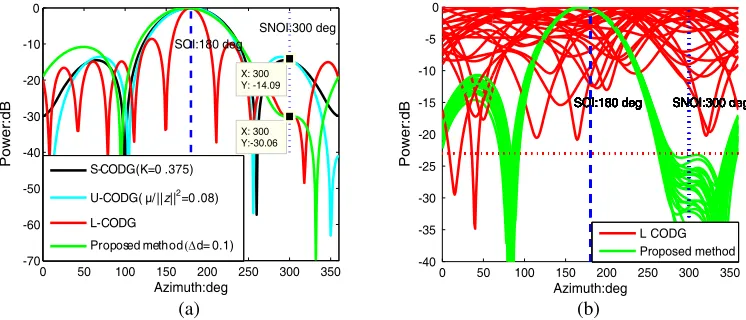
In order to analyze practical performance of the proposed method, assume a compact circular array model which consists of 11 idealized short vertical dipole elements. The array radius is 4 m, and working frequency is 12 MHz. SOI is from 180◦, and SNOI is from 300◦. Three virtual interference constraints are added to form a broaden null with −30 dB depth. Disturbance spacing is 10◦. Desired array efficiency should be above 24%. Make initial loading value Δd= 5×10−3 and incremental step δ = 10−3. By computation, when the total iteration number is 95 and final Δd= 0.1, specified efficiency is satisfied. With reference to Formula (2), the corresponding array sensitivity factor is 0.378, and directive gain is 17.7 dB. Fig. 1(a) shows corresponding beampatterns. Other patterns by S-CODG and U-CODG methods are drawn together to form contrast.

In order to present the comparative results better, Table 1 lists speciﬁc performance indicators. As can be seen, S/U-CODG methods satisfy the same array eﬃciency as the proposed method does. However, their sidelobe levels located at SNOI direction are much higher (−14.61 dB, −14.09 dB

0 50 100 150 200 250 300 350

-70 -60 -50 -40 -30 -20 -10 0

SOI:180 deg

X: 300 Y:-30.06

Azimuth:deg

Power:dB

SNOI:300 deg

X: 300 Y: -14.09

S-CODG(K=0 .375)

U-CODG( µ/||z||2=0 .08)

L-CODG

Proposed method(Δ d= 0.1)

(a)

0 50 100 150 200 250 300 350

-40 -35 -30 -25 -20 -15 -10 -5 0

Azimuth:deg

Power:dB

SOI:180 deg SNOI:300 deg

SOI:180 deg SOI:180 deg SOI:180 deg SOI:180 deg SOI:180 deg SOI:180 deg

L CODG Proposed method

(b)

(5)

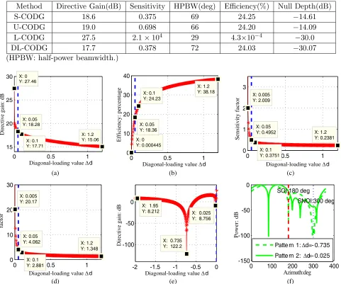
Table 1. Performance indicators (Δd= 0.1).

Method Directive Gain(dB) Sensitivity HPBW(deg) Eﬃciency(%) Null Depth(dB)

S-CODG 18.6 0.375 69 24.25 −14.61

U-CODG 19.0 0.698 66 24.20 −14.09

L-CODG 27.5 2.1×104 29 4.3×10−4 −30.0

DL-CODG 17.7 0.378 72 24.03 −30.07

(HPBW: half-power beamwidth.)

0 0.5 1

15 20 25 30

X: 1.2 Y: 15.06

Diagonal-loading valueΔ d

Directive gain: dB

X: 0.1 Y: 17.71 X: 0 Y: 27.46

X: 0.05 Y: 18.28

(a)

0 0.5 1

0 10 20 30 40

X: 0 Y: 0.000445

Efficiency: percentage

X: 0.1 Y: 24.23

X: 0.05 Y: 18.36

X: 1.2 Y: 38.18

(b)

0 0.5 1

0 1 2 3

X: 1.2 Y: 0.2381

Sensitivity factor

X: 0.1 Y: 0.3751 X: 0.005 Y: 2.009

X: 0.05 Y: 0.4952

(c)

0 0.5 1

0 10 20 30

X: 1.2 Y: 1.348

factor

X: 0.1 Y: 2.881 X: 0.005 Y: 20.17

X: 0.05 Y: 4.062

(d)

-2 -1.5 -1 -0.5 0

-100 -50 0

Directive gain: dB

X: 1.95

Y: 8.212 _{X: 0.025} Y: 8.756

X: 0.735 Y: 122.2

(e)

0 100 200 300 400

-150 -100 -50 0

Azimuth:deg

Power: dB

SOI:180 deg

SNOI:300 deg

Patte rn 1: Δd=- 0.735

Patte rn 2: Δd=- 0.025

(f)

Diagonal-loading valueΔ d Diagonal-loading valueΔ d

Diagonal-loading valueΔ d

Figure 2. Performance analysis. (a) Directivity corresponding to a given Δd. (d)η corresponding to a given Δd. (c) Sensitivity corresponding to a given Δd. (d) Q factor corresponding to a given Δd. (e) Directivity corresponding to a negative Δd. (f) Patterns under negative Δd

respectively), which verifies their limited anti-jamming performance. Although the pattern by L-CODG method has deep enough null level (−30.0 dB) at interference direction, its array efficiency (only 4.3×10−4) is far below specified value. Besides, its considerably high sensitivity indicator (2.1×104) also reflects that the pattern will be very unstable when confronting array uncertainty. For example, we add−35 dB (Standard Deviation 0.0178) random amplitude errors and 3◦ (Standard Deviation 0.0524) random phase errors into array model. Both meet independent Gaussian distribution. Fig. 1(b) shows corresponding patterns under 20 times Monte-Carlo tests. Obviously, the pattern by L-CODG has serious distortion while that of DL-CODG still keeps robust. Therefore, the proposed method makes a better tradeoff among efficiency, robustness and anti-jamming ability.

(6)

radiation eﬃciency is only 4.45×10−4%, which cannot be realized in practical engineering. When Δd <0, as shown in Fig. 2(e), array directivity is generally smaller than that of positive loading. In interval Δd ∈ [−1.1,−0.5], directive gain is negative, which means that mainlobe distortion occurs. Especially when Δd= −0.735, directive gain has minimum −122.2 dB, which even forms a deep null at desired SOI position. Corresponding beampattern is plotted in Fig. 2(f). Consequently, in order to keep high directive gain and avoid pattern distortion, positive loading value should be selected.

4. NUMERICAL METHOD 2 4.1. Theory and Implementation

As can be seen from above, virtual nulling techniques are suitable for high power interference, especially when SNOI comes from a concentrated direction. If interferences are more, and they present dispersion distribution, low sidelobe will produce more signiﬁcant suppression eﬀect. Corresponding mathematical expression can be written as:

min w w

H_(R_{+ Δ}_d_I)w_, _{subject to} _wH_a(_θ

0, φ0) = 1, |wHa(θi, φi)| ≤SLL (18)

where (θ0, φ0) denotes desired mainlobe position, and (θi, φi) belongs to speciﬁed sidelobe region. SLL

is speciﬁed maximum sidelobe level.

In order to solve the above problem, the following numerical iteration steps are adopted:

Step 1) Assume thatP virtual interferences (P ≥6) are located in speciﬁed sidelobe region. Set initial nulling constraints:

min w0 w0

H_(R_{+ Δ}_d_I)w

0, subject to w0Ha(θ0, φ0) = 1, |w0Ha(θi, φi)|=l0< SLL (19)

wherel0 denotes initial null depth which should be smaller thanSLL. According to Formula (17),

get initial weight vectorw0.

Step 2) Use weight vectorw0 to compute amplitude response and ﬁnd local maximumlj located at

(θj, φj) in each sidelobe (Boundary points cannot be ignored). Compute corresponding diﬀerence level betweenlj and SLL:

Δlj = lj

|lj|(SLL− |lj|) (20)

Step 3) Use the following constraints to compute step weight vector Δw:

min

Δw Δw

H_(R_{+ Δ}

dI)Δw, subject to ΔwHa(θ0, φ0) = 0, |ΔwHa(θj, φj)|= Δlj (21)

Step 4) Update weight vector: w=w0+ Δw. Compute amplitude response in sidelobe region. If

response level is less than speciﬁedSLL, iteration ends. Otherwise, return to Step 2).

4.2. Numerical Examples and Analysis

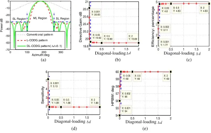
Still use the array model in Section 3: 11-element circular array, 4 m array radius, 12 MHz working frequency. Assume mainlobe direction as 180◦. Specified sidelobe region is located in interval [0◦,100◦][260◦,360◦], and desired maximum sidelobe level is SLL ≤-30 dB. In order to satisfy the constraints, we set 6 virtual interferences (20◦,60◦,100◦,260◦,300◦,340◦) which are evenly distributed in sidelobe region. Diagonal loading value Δd = 0.1 and initial null depth is −55 dB. After several iterations, array pattern will become stable, which is shown in Fig. 3(a). As can be seen, L-CODG and the proposed method are both favorable on sidelobe level index. However, on array efficiency, L-CODG is only 0.287%, and the proposed method is 4.8%. On sensitivity, L-CODG is 31.66, and the proposed method is 1.89. Apparently, the proposed method has higher array efficiency and better robustness.

(7)

0 100 200 300 -70 -60 -50 -40 -20 -10 0

SL Region ML Region SL Region

Azimuth:deg

Power:dB

Conventi onal patte rn

L-CODG patte rn

DL-CODG patte rn( Δd=0 .1)

(a)

0 0.5 1 1.5 2

19.8 20 20.2 20.4 20.6 20.8 21 X: 2 Y: 19.89 X: 0.5 Y: 19.89 X: 0.05 Y: 19.92 X: 0.001 Y: 20.83

Directive Gain: dB

d

(b)

0 0.5 1 1.5 2

1 2 3 4 5 X: 2 Y: 4.83 d Efficiency: percentage X: 0.5 Y: 4.83 X: 0.05 Y: 4.8 X: 0.002 Y: 3.11 X: 0.001 Y: 1.77

0 0.5 1 1.5 2

1 2 3 4 5 6 X: 2 Y: 1.88 d Sensitivity X: 0.5 Y: 1.88 X: 0.05 Y: 1.89 X: 0.001 Y: 5.13 (d)

0 0.5 1 1.5 2

54 55 56 57 58 59 60 X: 2 Y: 60 d HPBW: deg X: 0.5 Y: 60 X: 0.05 Y: 60 X: 0.002 Y: 56 X: 0.001 Y: 54 (e) (c) Δ Δ Δ _Δ Diagonal-loading Diagonal-loading Diagonal-loading Diagonal-loading

Figure 3. Performance analysis(SLL=−30 dB). (a) Pattern contrast. (b) Directivity corresponding to a given Δd. (c) η corresponding to a given Δd. (d) Sensitivity corresponding to a given μ. (e) HPBW corresponding to a given Δd.

Table 2. Performance indicators (Δd= 0.1).

SpeciﬁedSLL(dB) Method Directive Gain (dB) Sensitivity HPBW (deg) Eﬃciency(%)

−15 L-CODG 20.37 2499 54 0.004

DL-CODG 22.17 9.7 48 0.935

−25 L-CODG 21.47 104.3 50 0.087

DL-CODG 19.82 1.53 60 5.95

−35 L-CODG 21.7 40.54 50 0.22

DL-CODG 19.37 1.32 62 6.862

−40 L-CODG 21.74 78.68 49 0.12

DL-CODG 18.95 1 64 9.06

−45 L-CODG 21.76 104 48 0.087

DL-CODG 18.62 0.81 66 11.24

(HPBW: half-power beamwidth.)

eﬃciency 0.287% and minimum sensitivity 31.66, which is still worse than the proposed method on condition ofSLL=−15 dB.

In addition to reducingSLL level, choosing suitable loading value Δdis also helpful in improving array efficiency and robustness, which can be verified in Figs. 3(b)–3(e). As can be seen, when Δd ∈ [0,0.005], increasing loading value will have significant effect on array performance. Efficiency increases from 1.77% to 4.8%, and sensitivity decreases from 5.13 to 1.89. When Δd≥0.05, the change trend of each indicator will be flat. When Δd≥0.5, array performance will be no longer improved as Δdincreases.

(8)

5. CONCLUSION

In this work, a set of simple superdirective pattern synthesis methods are proposed. By adding virtual interferences and diagonal loading value as constraints, an array can make a better tradeoﬀ among directive gain, eﬃciency and anti-jamming performance. The proposed methods adopt numerical iteration solution and have simple parameter selection criteria, which is convenient for engineering realization.

ACKNOWLEDGMENT

This work is supported by the Fundamental Research Fund for the Central Universities under grant 20420150029 and by the Natural Science Foundation of Hubei Province under grant 2014CFA039. The authors would also like to thank the reviewers for many helpful comments and suggestions, which have enhanced the quality and readability of this paper.

REFERENCES

1. Sanzgiri, S. M. and J. K. Butler, “Constrained optimization of the performance indices of arbitrary array antennas,” IEEE Transactions on Antennas and Propagation, Vol. 19, No. 4, 493–497, 1971. 2. Schelkunoﬀ, S. A., “A mathematical theory of linear arrays,” Bell System Technical Journal,

Vol. 22, No. 1, 80–107, 1943.

3. Barrick, D. E. and P. M. Lilleboe, “Circular superdirective receive antenna arrays,” Patent No.: US 6,844,849 B1, Jan. 18, 2005

4. Ma, Y. L., Y. X. Yang, Z. Y. He, et al., “Theoretical and practical solutions for high-order superdirectivity of circular sensor arrays,” IEEE Transactions on Industrial Electronics, Vol. 60, No. 1, 203–209, 2013.

5. Yaru, N., “A note on super-gain antenna arrays,”Proceedings of the IRE, Vol. 39, No. 9, 1080–1085, 1951.

6. Newman, E. H., J. H. Richmond, and C. H. Walter, “Superdirective receiving arrays,” IEEE Transactions on Antennas and Propagation, Vol. 26, No. 5, 629–639, 1978.

7. Dawoud, M. and A. Anderson, “Design of superdirective arrays with high radiation eﬃciency,” IEEE Trans. on Antennas and Propagation, Vol. 26, No. 6, 819–823, 1978.

8. Zhou, Q. C., H. T. Gao, H. J. Zhang, et al., “Robust superdirective beamforming for HF circular receive antenna arrays,” Progress In Electromagnetics Research, Vol. 136, 665–679, 2013.

9. Zhang, H. J., H. T. Gao, Q. C. Zhou, et al., “A novel digital beamformer applied in vehicle mounted HF receiving device,”IEICE Electronics Express, Vol. 11, No. 2, 1–8, 2014.

10. Zhang, H. J., H. T. Gao, L. Zhou, et al., “Robust superdirective beamforming under uncertainty set constraint,”Progress In Electromagnetics Research C, Vol. 59, 59–69, 2015.

11. Zhou, Q. C., H. T. Gao, H. J. Zhang, et al., “Superdirective beamforming with interferences and noise suppression via second-order cone programming,”Progress In Electromagnetics Research C, Vol. 43, 255–269, 2013.

12. Yang Y. X., Y. Wang, Y. L. Ma, et al., “Experimental study on robust supergain beamforming for conformal vector arrays,”Oceans. IEEE, 1–5, 2013.

13. Olen, C. A. and R. T. Compton, “A numerical pattern synthesis algorithm for arrays,” IEEE Transactions on Antennas and Propagation, Vol. 38, No. 10, 1666–1676, 1990.

14. Tseng, C. Y. and L. J. Griﬃths, “A simple algorithm to achieve desired patterns for arbitrary arrays,” IEEE Transactions on Signal Processing, Vol. 40, No. 14, 2737–2746, 1992.

15. Shi, Z. and Z. Feng, “A new array pattern synthesis algorithm using the two-step least-squares method,”IEEE Signal Processing Letters, Vol. 12, No. 3, 250–253, 2005.