University of Windsor University of Windsor
Scholarship at UWindsor
Scholarship at UWindsor
Electronic Theses and Dissertations Theses, Dissertations, and Major Papers
2010
Mobile robot localization failure recovery
Mobile robot localization failure recovery
Sepideh Seifzadeh
University of Windsor
Follow this and additional works at: https://scholar.uwindsor.ca/etd
Recommended Citation Recommended Citation
Seifzadeh, Sepideh, "Mobile robot localization failure recovery" (2010). Electronic Theses and Dissertations. 7867.
https://scholar.uwindsor.ca/etd/7867
MOBILE ROBOT LOCALIZATION FAILURE RECOVERY
by
Sepideh Seifzadeh
A Thesis
Submitted to the Faculty of Graduate Studies through School of Computer Science in Partial Fulfillment of the Requirements for the Degree of Master of Applied Science at the
University of Windsor
Windsor, Ontario, Canada
2010
1*1
Library and Archives CanadaPublished Heritage Branch
395 Wellington Street Ottawa ON K1A 0N4 Canada
Bibliotheque et Archives Canada Direction du
Patrimoine de i'edition 395, rue Wellington Ottawa ON K1A 0N4 Canada
Your file Votre reference ISBN: 978-0-494-62736-5 Our file Notre reference ISBN: 978-0-494-62736-5
NOTICE: AVIS:
The author has granted a
non-exclusive license allowing Library and Archives Canada to reproduce, publish, archive, preserve, conserve, communicate to the public by
telecommunication or on the Internet, loan, distribute and sell theses
worldwide, for commercial or non-commercial purposes, in microform, paper, electronic and/or any other formats.
L'auteur a accorde une licence non exclusive permettant a la Bibliotheque et Archives Canada de reproduire, publier, archiver, sauvegarder, conserver, transmettre au public par telecommunication ou par I'lntemet, preter, distribuer et vendre des theses partout dans le monde, a des fins commerciales ou autres, sur support microforme, papier, electronique et/ou autres formats.
The author retains copyright ownership and moral rights in this thesis. Neither the thesis nor substantial extracts from it may be printed or otherwise reproduced without the author's permission.
L'auteur conserve la propriete du droit d'auteur et des droits moraux qui protege cette these. Ni la these ni des extraits substantiels de celle-ci ne doivent etre imprimes ou autrement
reproduits sans son autorisation. In compliance with the Canadian
Privacy Act some supporting forms may have been removed from this thesis.
Conformement a la loi canadienne sur la protection de la vie privee, quelques
formulaires secondaires ont ete enleves de cette these.
While these forms may be included in the document page count, their removal does not represent any loss of content from the thesis.
Bien que ces formulaires aient inclus dans la pagination, il n'y aura aucun contenu manquant.
• + •
Declaration of Co-Authorship/Previous
Publications
In all cases, the key ideas, primary contributions, experimental designs, data analysis
and interpretation, were performed by the author, and the contribution of co-authors
was primarily through the provision of corrections and constructive criticism. I am
aware of the University of Windsor Senate Policy on Authorship and I certify that
I have properly acknowledged the contribution of other researchers to my thesis,and
have obtained written permission from each of the co-author (s) to include the above
material(s) in my thesis. I certify that, with the above qualification, this thesis, and
the research to which it refers, is the product of my own work. This thesis includes
1 original paper that has been previously published, as follows:
Authors
S. Seifzadeh,
D. Wu, Y.
Wang
Publication title/full citation
"Cost-effective Active Localization Technique
for Mobile Robots"; IEEE International
Confer-ence on Robotics and Biomimetics, 2009
Publication
status
Published
I hereby certify that I have obtained a written permission from the copyright
owner(s) to include the above published material(s) in my thesis. I certify that the
above material describes work completed during my registration as graduate student
I certify that, to the best of my knowledge, my thesis does not infringe upon
anyone's copyright nor violate any proprietary rights and that any ideas, techniques,
quotations, or any other material from the work of other people included in my
thesis, published or otherwise, are fully acknowledged in accordance with the standard
referencing practices. Furthermore, to the extent that I have included copyrighted
material that surpasses the bounds of fair dealing within the meaning of the Canada
Copyright Act, I certify that I have obtained a written permission from the copyright
owner(s) to include such material(s) in my thesis and have included copies of such
copyright clearances to my appendix. I declare that this is a true copy of my thesis,
including any final revisions, as approved by my thesis committee and the Graduate
Studies office, and that this thesis has not been submitted for a higher degree to any
Abstract
Mobile robot localization is one of the most important problems in robotics.
Localiza-tion is the process of a robot finding out its locaLocaliza-tion given a map of its environment.
A number of successful localization solutions have been proposed, among them the
well-known and popular Monte Carlo localization method, which is based on particle
niters. This thesis proposes a localization approach based on particle filters, using
a different way of initializing and resampling of the particles, that reduces the cost
of localization. Ultrasonic and light sensors are used in order to perform the
experi-ments. Monte Carlo Localization may fail to localize the robot properly because of
the premature convergence of the particles. Using more number of particles increases
the computational cost of localization process. Experimental results show that,
ap-plying the proposed method robot can successfully localize itself using less number of
Dedication
Acknowledgements
I would like to express my gratitude to all those who gave me the possibility to
complete this thesis. I am grateful to each of my thesis committee members, whose
individual and collaborative efforts and guidance have made this endeavour an
un-forgettable experience, characterized by academic and professional growth and
self-discovery. I wish to thank my advisor, Dr. Dan Wu for his constant support during
my thesis work and through completion of my degree requirements and research.
Without his support, this thesis could not have been completed. I also would like to
thank members of my master committee, Dr. Scott Goodwin, School of Computer
Science, Dr. Chunhong Chen, Department of Electrical and Computer Engineering,
for being in my committee, and their constructive criticism, helpful advices, and
Table of C o n t e n t s
Page
Declaration of Previous Publications iii
Abstract v Dedication vi Acknowledgements vii
List of Tables x List of Figures xi Chapter
1 Introduction 1 1.1 Outline 2
2 Background Knowledge 4 2.1 Probabilistic Robotics 4
2.1.1 Map Representation 6
2.2 Mobile Robot Localization and Localization Algorithms 7
2.2.1 The Bayes Filter and Kalman Filter Algorithms 7
2.3 Categories of Localization Problems 9
2.3.1 Whether the Initial Pose is Known to the Robot 9
2.3.2 Weather or Not the Robot's Effectors are Controlled 10
2.3.3 Type of Environment 10
2.3.4 Number of Mobile Robots 10
2.4.1 Monte Carlo Localization 11
2.4.2 Implementation of MCL 12
2.5 Kidnapped Robot Problem 15
2.6 Related Works 16
3 Mobile Robot Localization Failure Recovery 19
3.1 Motivation of Our Method 19
3.2 The Proposed Method 20
3.2.1 Problem Statement 20
3.2.2 Description of the Proposed Method 20
3.2.3 Initialization of the Particles 22
3.2.4 Resampling the Particles 22
3.2.5 Kidnapped Robot Problem 24
4 Implementation and Experimental Results 26
4.1 Implementation Details 26
4.1.1 Hardware Platform and Programming Environment 26
4.2 Experimental Results 29
4.2.1 Simulation Results 29
4.2.2 Experiments Using Real Robot 36
4.2.3 Discussion and Comparison 42
5 Conclusion and Future Work 48
5.1 Conclusion 48
5.2 Future Work 49
List of Tables
2.1 Bayes Filter Algorithm 8
2.2 Markov-localization Algorithm 9
2.3 MCL Algorithm 18
4.1 Comparison of performance of the proposed method and traditional
MCL, for kidnapping problem in simulation environment without
ob-stacle 34
4.2 Comparison of performance of the proposed method and traditional
MCL, for kidnapping problem in simulation environment with obstacle. 34
4.3 Comparison of performance of the proposed method and traditional
MCL, for kidnapping problem in real environment without obstacle. . 40
4.4 Comparison of performance of the proposed method and traditional
MCL, for kidnapping problem in real environment with obstacle. . . . 40
List of Figures
2.1 Probabilistic generation of robot kinematic; (a) A p a t h of moving
for-ward; (b) A p a t h of more complicated motion command [25] 13
2.2 Odometry model 14
3.1 Proposed algorithm 21 3.2 Initialization: (a) Initialization in regular MCL; (b) Beginning of the
local-ization process; (c) Initiallocal-ization of the particles base on sensor readings. . 23 3.3 Failure recovery: (a) Mobile robot is localized; (b) Kidnapped robot
prob-lem; (c) Robot is recovered and re-localized 25
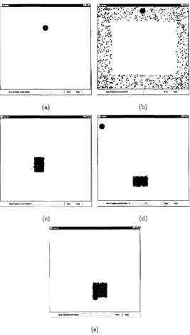
4.1 LEGO MINDSTORM NXT 28 4.2 Localization in the first simulation environment : (a) Beginning of
localiza-tion process; (b) Initializalocaliza-tion of particles; (c) Mobile robot is localized; (d)
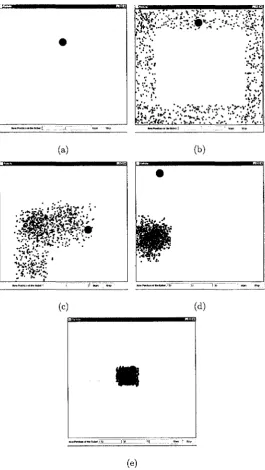
Robot is kidnapped; (e) Localization failure recovery. 32 4.3 Localization in the Second simulation environment : (a) Beginning of
local-ization process; (b) Initiallocal-ization of particles; (c) Robot is kidnapped; (e)
Localization failure recovery. 33 4.4 Simulation environment without obstacle 34
4.8 Real localization environment with obstacle: (a) Localization
environ-ment with obstacle; (b) NXT is located in a random place; (c)
Initial-ization of particles; (d) InitialInitial-ization of the particles based on sensor
data 38
4.9 Real localization environment with obstacle: (a) Particles trying to
localize the robot; (b) Mobile robot trying to localize itself; (c) Particles
are localizing the robot; (d)Robot is localized 39
4.10 Real environment without obstacle 41
4.11 Real environment with obstacle 41
4.12 Localization using MCL in environment without obstacle, (a) Particles
are generated randomly; (b) Robot is localized; (c) Robot is being
kidnapped 46
4.13 Localization using MCL in environment with an obstacle, (a)
Initial-ization of the particles; (b) Mobile robot is localized; (c) Robot is being
Chapter 1
Introduction
Localization is the most fundamental problem to provide a mobile robot with
au-tonomous capabilities. Almost all tasks of mobile robots require a robot to have
accurate knowledge about its location such as in Robotic Soccer. Mobile robot
local-ization [4] is the problem of determining the position of a mobile robot relative to a
given map of the environment and using the sensor data. It is often called position
estimation or position tracking [13]. Let I = (x, y, 8) denote a location, the robot
pose is usually given by three variables, robot's two location coordinates in the plane
(x, y) and robot's orientation 9. In probabilistic robotics, the notion of belief bel(Lt)
is used to reflect the robot's internal knowledge about the state of the environment.
The state cannot be measured directly. It must be inferred from the measurement
data and control data.
Monte Carlo Localization which is based on Particle filters and represents the
belief bel(xt) of the mobile robot by particles is one of the localization algorithms
and has already become one of the most popular localization algorithms in robotics.
It is easy to implement, and tends to work well across a broad range of localization
problems. Most of the existing approaches can not recover from localization failure
and kidnapped robot problems. Therefore we need a method to localize the robot
The number of samples to be used is important, since using more number of particles
will increase the cost of localization.
The proposed method is an improved approach to localize the mobile robot. It
recovers the robot from localization failures with high probability. It has some
dif-ferences from the regular MCL algorithm, modified initialization step and modified
resampling step that helps to reduce some steps of localization and the cost of
lo-calization, and re-generating particles in the case of localization failure that helps
to prevent the robot from failure in kidnapped robot problem situation. Applying
the proposed method, it is expected that robot localizes itself with a high probability
with lower cost. In terms of realization proposed method is much easier to implement,
since particles are not generated from the very beginning and the cost of localization
and computational costs are therefore decreased. Localization is done faster and more
accurate with the use of less number of particles.
This thesis is only concerned on the localization problems in indoor environments,
particularly in small-scale room with robot equipped with low-cost sensors. The
most important aspect of the proposed method is to help the robot to recover from
localization failure.
1.1 Outline
This remainder of the thesis is organized as follows.
Chapter 2 consists background knowledge. This chapter is focused on the
materi-als that the proposed approach is based on. First, we will introduce the uncertainty
in robotics and provide a comprehensive overview of probabilistic robotics. Then
description of basic probabilistic concepts are given. Monte Carlo localization which
is one of the methods of localization and is the fundament of the proposed method
is given in more details and finally there is a brief review of the related works in the
details. First the statement of the problem and the general description of our method,
and then the comparison of the proposed method with the existing methods which
is followed by the discussion of the experimental results in chapter 4. Experiments
are performed in different environments to verify the performance of the proposed
approach. The detailed information of the implementation and the experimental
re-sults are discussed. Finally, we conclude this research work with discussion of possible
C h a p t e r 2
B a c k g r o u n d Knowledge
This chapter provides the background knowledge which the proposed method is based
on. First, we present basic idea of probabilistic robotics, followed by the definition of
mobile robot localization and localization algorithm. Then, Monte Carlo localization
(MCL) algorithm is explained since it is one of the most important probabilistic
algorithms for mobile robot localization and also the foundation of the proposed
method followed by implementations of MCL. Then, we describe kidnapped robot
problem which is a problem that may occur during the localization of the mobile
robot and will result in localization failure. The summary of the related work to date
is given at the end.
2.1 Probabilistic Robotics
Unlike the previous approaches relying on a single best guess of what might be the
case; probabilistic algorithms describe the robot and the environment using random
variable. In particular, there are two basic models involved in probabilistic robotics:
perception, the way sensor is processed, and action, the way robot behaves. By doing
so, probabilistic robotics provides a great way to accommodate the uncertainty that
comes from most robot practice. As a result, they perform excellent in the face of
In probabilistic robotics, we describe the robot and environments using the notion
of state, which can be defined as a collection of all aspects of the robot and its
environment that can impact the future [14]. The state variables that tend to change
over time will be called dynamic state, such as walking people around the robot. The
state that does not change is called static state, such as location of walls in buildings.
The state also involves variables related to robot itself, such as its pose, velocity and
so on. In this thesis, state is denoted as x; the state at time t is denoted as xt.
Time defined here is discrete. That is, all states can be described at discrete time
steps t = 0,1,2,.... The initial state of the robot will be denoted as time t = 0.
For robot action, the state includes variables for the configuration of the robot's
actuators. The location and features of surrounding objects in the environment are
also state variables. An object may be a chair, a box or a wall. Features of these
objects may be their texture or color. The location of objects in the environment is
static in this thesis. Many other variables that may impact a robot's operation can
be state variables as well. The list of all possible state variables is endless. Typical
state variable used in this thesis is the robot pose that includes robot's location and
orientation relative to a global coordinate system. Strictly speaking, mobile robots
have six such state variables, three for Cartesian coordinates, and three for angular
orientation. But for robots defined in planar environments, the pose is usually given
by three variables, two location coordinates in the plane and the heading direction.
There are two fundamental types of interaction between a robot and its
environ-ment: sensor measurements and control actions [14].
Sensor measurement is the process in which the robot obtains the information
about its environment through sensors. Control actions include the robot motion and
the manipulation of objects in the environment. In accordance with two kinds of
environment interactions, robot receives two different streams of data: measurement
data and control data (also referred to as movement data or motion data).
to time t and zt to denote the measurement data at time t. For movement data,
we use ui-t to denote all movement data from time 1 to time t and ut to denote
movement data at time t. For these two kinds of data, localization algorithms based
on probabilistic robotics [14] have two separate components to process them. One
is the measurement model, and the other is the motion model. The measurement
model p(zt \ xt) is the conditional probability of zt at the state xt . The motion
model comprises the state transition probability p(xt | ut, xt~i), which describes the
posterior distribution after incorporating the motion data ut at xt-\.
2.1.1 Map Representation
Mobile robot localization problem assumes that robot is given a map in advance. If
the map of the environment is not given to the mobile robot then the robot should
build the map while trying to localize itself in the environment and that is called
SLAM (simultaneous localization and mapping). The map specifies the environment
in which measurements are generated. Formally, a map m is a list of objects in the
environment with their properties. M = m\, m2, , mn.
If the map of the environments is not given to the mobile robot, then the robot
can calculate the posterior over maps given the data. p(m \ z\-t, Xi:t). Let m; denote
the grid cell with index i. An occupancy grid map partitions the space into finitely
many grid cells: m = ^2 i. Each m; has attached to it a binary occupancy value,
which specifies whether a cell is occupied or free. We will write " 1" for occupied and
"0" for free. The notation p(m, = 1) or p{mi) will refer to a probability that a grid
2.2 Mobile R o b o t Localization a n d Localization
Algorithms
2.2.1 The Bayes Filter and Kalman Filter Algorithms
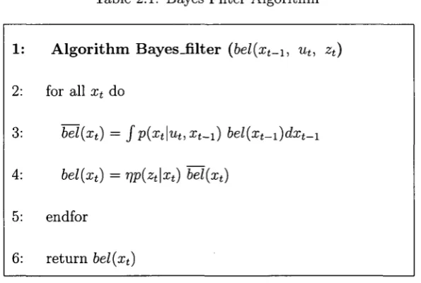
The most general algorithm for the state estimation is Bayes filter [14]. It calculates
the posterior probability bel(xt) according to the measurement and control data as
follows:
bel(a;t) = p(xt | z0:U u0-t)
where xt denotes the robot pose (x, y, 9) at time t, z0:t = ZQ, Z\, ... , zt denotes
the sensor readings up to t, and uo:t — uo, u\, ... , ut is the control data changing the
state of the world. The input of Bayes filter is the belief bel(xt-i) at time t — 1, along
with the most recent control ut, and the most recent measurements zt. The output is
the belief bel(xt) at time t. The measurements of sensors and the control information
are corrupted with noise. In order to deal with these uncertainties, Bayes filter is
conducted in two phases: prediction phase (line 3 of the algorithm), it processes the
movement data ut , and calculate the state xt using the prior belief over state xt-\
and the movement ut. The second step (line 4 of the algorithm) is called update
phase. It processes the measurement data zt, and incorporate it into bel(x(). But
the result be\(xt) may not integrate to 1, so it uses the normalization constant r] to
normalize the result bel(xt).
The Kalman filter technique is commonly used in local localization. The robot
estimates its pose continuously by counterbalancing the odometric error using the
sensor data. Therefore, if the initial pose is accurate and sensor error is small, the
Kalman filter can provide efficient, accurate, and continuous localization result.
Mobile robot localization is the problem of determining the pose of a robot in a
given map of the environment. Localization algorithms are variant implementations
Table 2.1: Bayes Filter Algorithm
1:
2:
3:
4:
5:
6:
Algorithm Bayes_filter (6e/(xf_i, ut, zt)
for all xt do
bel(xt) = J'p(xt\ut, xt^i) bel(xt-i)dxt-i
bel(xt) = r]p(zt\xt) bel(xt)
endfor
return bel(xt)
of multiple beliefs to allow a robot to infer its position and orientation. Table 2.1
shows Bayes filter algorithm.
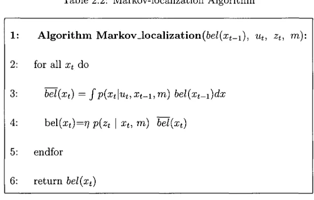
Localization algorithms based on probabilistic theory are variants of Bayes filter.
In the context of mobile robot localization, Bayes filters is also known as Markov
localization [14], [2]. Table 2.2 shows the basic algorithm of Markov localization.
It is derived from the Bayes filter algorithm with map m of the environment also
as input (line 1 of the algorithm). The map m is important in the measurement model
p(zt | xt, m) (line 4 of the algorithm), and is also used in the motion model p(xt \
ut, Xt-i, m) (line 3 of the algorithm). The same as Bayes filter, Markov localization
calculates the probabilistic belief bel(xt) at time t from time t — 1 recursively.
Markov localization or Bayes filter is independent of the representation of state
space [14], and it can be implemented by using different state representation methods,
for example, histogram filter and particle filter. Histogram filter decomposes the state
space into finite regions and represents the cumulative posterior for each region by
a single probability value [24]. Particle filter [11] approximates the posterior by a
Table 2.2: Markov-localization Algorithm
1: A l g o r i t h m Markov_localization(6e/(xt_1), ut, zt, m):
2: for all xt do
3: bel(xt) = Jp(xt\ut,xt-1,m) bel(xt-i)dx
4: bel(ort)=T7 p(zt \ xt, m) bel(xt)
5: endfor
6: return bel(xt)
randomly from the posterior [23], [1].
2.3 Categories of Localization P r o b l e m s
Localization problem can be classified based on 1) whether the initial pose is known
to robot or not, 2) weather or not the robot's effectors are controlled, 3) type of the
environment, and 4) the number of robots.
2.3.1 Whether the Initial Pose is Known to the Robot
Localization can be divided into two parts, global position estimation [7] and local
position tracking [21], [22], [14]. Global position estimation is the ability to determine
the robot's position in a previously learned map, given no other information than that
the robot is somewhere in the map. Once a robot has been localized in the map, local
2.3.2 Weather or Not the Robot's Effectors are Controlled
Passive localization approaches, do not exploit the opportunity to control the robot's
effectors during localization. In passive localization, the localization module only
works as an observer on the robot. Active localization provides setting the robot's
motion direction and determining the pointing direction of the sensors during
local-ization. The control of the robot does not include facilitating locallocal-ization. The robot
might move randomly or do its own jobs. Active localization algorithms control the
robot in order to minimize the localization error or the costs that risk a poorly
local-ized robot moving into dangerous places. Active approaches for localization problem
usually have much better localization results than passive ones, such as coastal
navi-gation.
2.3.3 Type of Environment
Environments can be static or dynamic. In static environment, only the robot moves
and all other objects stay at the same location. In dynamic environments, other than
robot, the location or configuration of other objects change over time.
2.3.4 Number of Mobile Robots
The last class of the localization problem is characterized by the number of robots
included: single-robot localization and multi-robot localization. In single robot case,
all data only need to be collected on a single robot platform, and no communication
issue comes in this problem. The multi-robot localization problem is brought by a
group of robots. The issue of multi-robot localization arises from the representation
of beliefs and the nature of the communication between them.
The most important characteristics of the mobile robot localization problems are
covered in these four categories. In this thesis, we deal with global localization of
2.4 M o n t e Carlo Localization Algorithm and its
I m p l e m e n t a t i o n
2.4.1 Monte Carlo Localization
As described in previous section, Kalman niters offer an elegant and efficient algorithm
for localization. However, the plain Kalman filters is inapplicable to global localization
problems due to the restrictive nature of the belief representation. In contrast to
Kalman filtering based techniques; MCL is able to represent multi-modal distributions
and therefore can globally localize a robot.
Monte Carlo Localization (MCL) takes a new approach to represent uncertainty
in mobile robot localization, instead of describing the state space by a probability
density function; represents it by maintaining a set of samples that are randomly
drawn from it. Monte Carlo methods are used to update this density representation
over time. MCL algorithm is the most popular approach to date, since it is easy to
implement, and works well across a broad range of localization problems. MCL is
applied to both global and local localization problems. MCL algorithm is shown in
Table 2.3 [14].
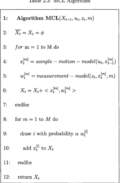
Table 2.3 shows the basic MCL algorithm, which is obtained by substituting the
appropriate probabilistic motion and perceptual models into the algorithm particle
filters. The basic MCL algorithm represents the belief bel(xt) by a set of M particles
Xt = xt ,xt, ...,xt . Lines 4 in the algorithm (Table 2.3) samples from the motion
model, using particles from present belief as starting points. The beam measurement
model is then applied in line 5 to determine the importance weight of that particle.
The initial belief bel(xo) is obtained by randomly generating M such particles from
the prior distribution p(x0), and assigning the uniform importance factor M_ 1 to
each particle. As the robot gets sensor measurements line 5 of the algorithm, MCL
the resampling step, and after incorporating the robot motion (line 4). This leads to
a new particle set with uniform importance weights, but with an increased number
of particles near the three likely places. The new measurement assigns non-uniform
importance weights to the particle set. At this point, most of the cumulative
prob-ability mass is centered on the second door, which is also the most likely location.
Further motion leads to another resampling step, and a step in which a new particle
set is generated according to the motion model. The particle sets approximate the
correct posterior, as would be calculated by an exact Bayes filter [14].
We have used odometry motion model as the basis for calculating the robot's
motion over time. Odometry motion model is commonly obtained by integrating
wheel encoders information. In the updating part according to the sensor reading the
weight of the particles will be updated. After updating, there is a resampling step
and then the summation of the weights of all particles should be equal to one.
2.4.2 Implementation of MCL
We will describe the implementation of MCL algorithm, in details below.
(a) Motion Model
Within the framework of MCL, motion model corresponds to the step sampling
from the state transition distribution p(xt \ ut, £t-i), which generates a hypothetical
state xt based on the particle set £t_i and the control ut. The motion model plays
an essential role in the prediction step of MCL.
The robot motion of probabilistic robotics conforms to the fact that the outcome
of a control is uncertain, because of the control noise or un-modeled effects. Therefore,
the outcome of a control will be represented by a posterior probability. The robot
motion, formally kinematics, is the calculating of the effect of control actions on the
configuration of a robot. The configuration of a mobile robot is commonly described
by three variables, referred as pose (x, y, 6). The pose without orientation is robot's
of the state transition model p(xt | ut, xt-\) in mobile robotics. The xt and xt-\ are
both robot poses and ut is a motion command. This model describes the posterior
distribution over states of kinematic when the motion command ut is executed at
Xt-\. Fig. 2.1 shows two examples of kinematic model for a mobile robot controlled
in a planar environment with the robot's pose initialed as xt-\. The shaded area
shows the distribution p(xt | ut, xt-i): the darker a pose, the more likely it is for the
robot to be at that location.
urn.
Figure 2.1: Probabilistic generation of robot kinematic; (a) A path of moving for-ward; (b) A path of more complicated motion command [25].
There are two common probabilistic motion models for mobile robots: velocity
motion model and odometry motion model. Velocity motion model assumes robot
is controlled through two velocities, a rotational and a translational velocity; and
odometry motion model assumes we have access to odometry information, which is
commonly obtained by integrating wheel encoder information. Velocity motion model
calculates the probability p(xt | ut, xt-i) of being at xt after executing the control ut
at the state xt-\. It assumes that the control is carried out for the fixed short time
duration t. Odometry motion model is used in our proposed method.
The odometry information consists of the distance a robot passed and the angle
a robot rotated. Most of the commercial robots provide odometry using kinematic
information. NXT has wheel encoders to obtain odomety information. Practical
ex-perience suggests that odometry is usually more accurate than velocity. In odometry
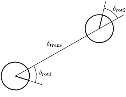
followed by a translation and a second rotation shown in Fig. 2.2 [14]. Both the turns
and translation suffer noisy, such as drift and slippage.
Figure 2.2: Odometry model
In Fig. 2.2 the robot motion in the time interval (t — l,t] is approximated by a
rotation 5rot\, followed by a translation 6trans a nd a second rotation 8Tot2- The turns
and translation are noisy.
(b) Measurement Model
Another important model in probabilistic robotics is the measurement model. The
probabilistic models of sensor measurements p(zt | xt) are essential for the
measure-ment update step in MCL. Measuremeasure-ment models describe the formation process by
which sensor measurements are generated in physical world. Today's robots use a
variety of different sensors, such as tactile sensors, range sensors, or cameras.
Prob-abilistic robotics explicitly models the inherent uncertainty in sensor measurements.
NXT has ultrasonic sensor, touch sensor, light sensor and sound sensor. The
ultra-sonic sensor will return the distance of the NXT to objects. In our experiment, we
use the ultrasonic sensor measurements in order to recognize if NXT is close to wall
or any object in the environment and light sensor measurements to recognize
obsta-cles. Then, high weight will be assigned to the particles that are close to the sensor
are forward to the next step importance sampling.
(c) Resampling
Another important component of MCL is known as resampling or importance
sampling. In our experiment, the algorithm low variance sampling is chosen for
resampling. The basic idea of low variance sampler includes a sequential
stochas-tic process. Instead of choosing M random numbers and selecting those parstochas-ticles
that correspond to these random numbers, this algorithm computes a single random
number and selects samples according to this number but still with a probability
pro-portional to the sample weight. The algorithm showed in Table 2.3 selects particles
by repeatedly adding the fixed amount M — 1 to r and by choosing the particle that
corresponds to the resulting number. The while loop at step 8 stops when i is the
index of the particle such that the corresponding sum of weights exceeds U. Then the
particle is selected. The low variance sampler is very efficient. At the end, we count
the number of particles with zero weight and if the "num-zero" variable is equal to or
greater than half of total number of particles, then a new set of particles is generated.
In regular MCL when the particles can not localize the robot or in situation like
kidnapping there is no surviving particles near the location of the robot, there is no
chance for to robot to recover from failure. But in the extended works that are based
on MCL they inject random particles to the localization process. In this work when
we apply the MCL, we calculate the weight of particles; as soon as the weight of all
particles are zero then a new set of particles is initialized and randomly distributed
all over the environment.
2.5 Kidnapped Robot Problem
Kidnapped robot problem [6], [19], [20] is a variant of global localization problem. It
happens when a robot that is aware of its location is moved to another location of
than global localization problem. In global localization problem, robot knows that
it does not know where it is. In kidnapped robot problem, Robot might believe it
knows where it is, while it does not. It is commonly used to test a robot's ability to
recover from localization failures.
Most of MCL-based works suffer from the kidnapping problem, since this approach
collapses when the current estimate does not fit observations. There are several
exten-sions to MCL that solves this problem by adding random samples at each iteration.
2.6 R e l a t e d Works
Several authors have demonstrated different methods in the area of mobile robot
lo-calization. The most efficient ones are based on particle filters where the significant
advantage of particle filter is to globally localize the mobile robot. Fox et al.
intro-duces Monte Carlo Localization for mobile robot localization [1]. Later, they have
proposed a technique for active localization of mobile robots [2], [3], [10], [9].
In [12] combination of existing methods was used to increase the efficiency of
lo-calization, i.e., first global search is made then a local search is performed, in order
to reduce the probability of finding a local minimum and improving the stability and
accuracy of solutions near the optimum. Extended Kalman filter (EKF) is used to
limit the search ares, otherwise the genetic search becomes too costly from the
compu-tational point of view. EKF obtains a seed which is used to estimate a neighborhood,
where the true value of the state is located, then in this restricted area the most
accurate solution is searched. Genetic algorithm only works in restricted areas of the
solution space and as the result it is a fast optimization method. Fitness function
then focuses the search in a certain neighborhood around the previous estimate, if
the new generation contains a solution that produces an output that is close enough
or equal to the desired answer then the problem has been solved.
cluster of particles. Based on sensor readings, which enables the robot to estimate
some positions with higher probability instead of generating particles that are
ran-domly distributed all over the environment, they have initialized particles just in the
places that the robot will know it is most probable to be the true position. Genetic
algorithm is then employed to work on the clusters that have been generated to get
a unique estimate of the real position of the robot.
In [7] a multi-robot active localization technique is proposed based on CEAMCL.
Using CEAMCL, samples are clustered into species which will evolve according to
a co-evolutionary model derived from the competition of ecological species, and the
size of the species will adaptively change according to the state of the robot. In
this way, CEAMCL cannot only prevent premature convergence of MCL but also
improves its efficiency, so CEAMCL is selected for cooperative localization. In [8] a
t-test revealed that it is significantly better to apply the active approach than the
passive one for the global localization task. Kummerle et al. [8] have presented an
approach to active Monte Carlo localization with a mobile robot using MLS
(Multi-level surface) maps. The approach actively selects the orientation of the laser range
finder to improve the localization results. To speed up the entire process, a clustering
operation was applied on the particles and only evaluate potential orientations based
on these clusters. Their new proposed approach is able to increase the efficiency of the
localization by minimizing the expected entropy. In contrast to the former approaches
[8] focus on reducing the computational demands of the active localization. The goal
of this paper is to develop an active localization method which is able to deal with
Table 2.3: MCL Algorithm
1:
2:
3:
4:
5:
6:
7:
8:
9:
10:
11:
12:
Algorithm M.CL(Xt~i,ut, zt,m)
x
t=
x
t—
4>
for m = 1 to M do
x™ = sample — motion — model(ut, x™[)
tv™ = measurement — model(zt, x\ , m)
x
t
=x
t
+<
x[
r\w
[
r
]
>
endfor
for m = 1 to M do
draw i with probability a wf'
add xf to Xt
endfor
C h a p t e r 3
Mobile R o b o t Localization Failure
Recovery
The description of the proposed method can be found in this chapter.
3.1 Motivation of Our M e t h o d
Most of the existing approaches can not recover from localization failure and
kid-napped robot problem. Therefore we need a method to localize the robot with higher
probability and with the ability to recover the robot from kidnapping problem . The
number of samples to be used is important, since using more number of particles will
increase the cost of localization. Since almost all tasks of mobile robots require a
robot to have accurate knowledge about its location, we need a method to localize
the robot with higher probability and with the ability to be able to recover the mobile
robot from kidnapping problem or any type of localization failure with the use of less
3.2 T h e P r o p o s e d M e t h o d
3.2.1 Problem Statement
Localization is the most fundamental problem to provide a mobile robot with
au-tonomous capabilities, therefore the result of the localization task should be accurate
and reliable to provide the robot an accurate knowledge about its location. Most
of the existing approaches can not recover from localization failure, for example
kid-napped robot problem which is a variant of localization failure. Therefore we need a
method to localize the robot with higher probability and with the ability to recover
the robot from kidnapping problem. The number of samples to be used is important,
since using more number of particles will increase the cost of localization. Therefore,
in the proposed method, we are trying to localize the robot with less number of
par-ticles than the other methods in order to reduce the cost of localization and localize
the robot with higher probability to recover from the failure.
3.2.2 Description of the Proposed Method
The proposed method [15] is an improved approach to localize the robot. It recovers
the robot from localization failures with high probability. Proposed method is based
on Monte Carlo Localization and has two differences from the regular MCL algorithm,
first modified initialization step and second modified resampling step.
It has the ability to re-generate the particles in the case of localization failure.
Applying the proposed method, it is expected that robot localize itself with a high
probability with lower cost. Two main advantages of the method, first different way
of initializing the particles that helps to reduce some steps and the cost of
localiza-tion. Second a new resampling scheme to solve the kidnapped robot problem and
localization failures.
Robot gets sensor reading and moves
< C ^ '
do>20 J ^ >
Yes ^^~~~~-r~^^
Yes
Initializing the particles based on sensor reading
< '
Prediction, Updating Resampling the particles
Particle Checker ""'
Robot is localized
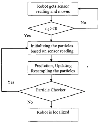
Figure 3.1: Proposed algorithm.
In the algorithm which is presented in Fig. 3.1; in first step, robot moves and
gets the value of its sensors. The value of the ultrasonic sensor which presents the
distance of the robot to the wall is presented as d0. Whenever the distance of the
robot to the wall (do) is less than 20cm then the particles are initialized; otherwise
robot continues moving and getting the sensor data. The distance of the robot to
wall is set to 20cm in order for robot to stop and turn since when doing the real
environment experiments, robot should have enough space in order to make a turn.
After initializing the particles, they are updating and resampling and their weights
changes as the robot moves. Particle-Checker step checks the condition of failure, if
the number of the particles with zero weight are greater than half of the total number
of particles then a new set of particles is generated.
The experiments are performed in order to evaluate the Error rate for the proposed
particles. The error rate is calculated as follows:
Number of times robot cannot localize itself successfully Error rate =
——-Total number or times
There is a comparison between Error rates for different experimental
environ-ments. In first two cases we calculate Error rate in the simulation environments with
obstacle and without obstacle. The last two sets of experiments are performed in the
real environment using NXT. In each set of experiments we run the program for MCL
and the proposed method 50 times and then draw a graph in order to compare the
Error rate for each case.
3.2.3 Initialization of the Particles
In this part there is a description of the differences of the initialization part in regular
MCL and the proposed method. In initialization part of regular MCL, as soon as
MCL runs; particles are generated. There is a uniform distribution of the particles all
over the environment. As shown in Fig. 3.2 (a) particles all have same weight at the
time of generation, bel(L0) is uniformly distributed to reflect the global uncertainty
of the robot.
In the proposed initialization technique, particles are not generated from the very
beginning as in Fig. 3.2 (b), they are generated based on sensor reading. As soon as
robot gets a sensor reading; particles are generated based on the most recent sensor
reading. The weight of the particles that are close to the location of the sensor reading
are higher than the other particles. Therefore particles are generated as some cluster
of particles rather than normally distributed all over the environment as shown in
Fig. 3.2 (c). Therefore, initial belief of the robot bel(L0) is not uniformly distributed.
3.2.4 Resampling the Particles
In this part there is a description of the differences of the resampling part of regular
! - *
•MfM
1 m •
• < ; v .
', kl
(a)
aissi
(c)
(b) ttmiL ... . JOA
when robot gets a sensor reading in the resampling part, particles are assigned new
weights based on new sensor reading. Particles are not re-generated if they do not
localize the robot correctly. In the proposed resampling technique, algorithm guesses
possible locations of the robot based on the sensor reading.
Using motion model this guess is corrected and particles will be assigned new
weights in the resampling step. As the extension of resampling step; if the weight
of most of the particles is zero, a new set of particles is generated based on the new
sensor reading. In other works done, some random particles are added to re-localize
the robot based on regular MCL. In this method, whenever robot knows that it is
lost, a new set of particles is generated based on the sensor reading.
3.2.5 Kidnapped Robot Problem
In the case of kidnapped robot problem, when robot is taken and placed in another
location of the environment; first it can not recognize that its location has been
changed and particles are predicted based on the previous information. When the
robot gets new sensor readings, since most of the particle's weights become zero,
based on new resampling method a new set of particles is generated to help the robot
localize itself and to figure out its true location.
The following figures illustrate the kidnapped robot situation. At first, when the
robot is taken and placed in another location of the environment it can not recognize
of being kidnapped. Particles continue their previous path, but after robot gets new
sensor readings and the weight of the particles is updated based on that, after the
"Particle-Checker" part which counts the number of the particles having zero weight,
if there is more than half of the particles with zero weight then a new set of particles
is generated based on the sensor reading. In Fig. 3.3 (a) robot is localized, but as
in Fig. 3.3 (b) it is being kidnapped and lost, and using the proposed resampling
technique the mobile robot realizes of being kidnapped and it successfully re-localize
•
•
. ?
»* ** * *•*" J" •«
•
(a)
mm-r
i
t M M f U W 4 i n r > * « i i ' «'i (b)
(c)
Chapter 4
Implementation and Experimental Results
The implementation of our proposed method and experiment results are described
in this chapter. Hardware platform and programming environment are presented at
first, followed by experimental results.
4.1 Implementation Details
4.1.1 Hardware Platform and Programming Environment
In 2006 Lego released MindStorms NXT. It includes a local file system on 256 KB
flash RAM. In our experiments we changed the original graphical operating system
inside NXT to LeJOS NX J operating system [28], [29], which is a tiny Java-based
operating system and is used for LEGO MINDSTORM NXT. NXT has four sensors,
sound sensor, light sensor, touch sensor and ultrasonic sensor.
Sound sensor: is the robot's ears. It allows LEGO MINDSTORMS NXT robot to
hear and is able to measure noise levels in both dB (decibels) and dBA (frequencies
around 36 kHz where the human ear is most sensitive), as well as recognize sound
patterns and identify tone differences.
Touch sensor: is robot's fingers. It reacts to touch and release, enabling NXT to
Intelligent.
Light sensor: detects light intensity. The Light sensor assists in helping the robot
to "see". Using the NXT Brick, it enables the robot to distinguish between light
and dark, as well as determine the light intensity in a room or the light intensity of
different colors. It can detect lights invisible to human eye such as infrared light.
Ultrasonic sensor: is robot's eyes, it enables the robot to see and detect objects,
also it is used to make the robot to avoid obstacles, and sense and measure distances,
and detect movement. It is able to measure distances from 0 to 255 centimeters with
a precision of ±3cm. The Ultrasonic sensor uses the same scientific principle as bats:
it measures distance by calculating the time it takes for a sound wave to hit an object
and return, just like an echo. Large sized objects with hard surfaces return the best
readings. Objects made of soft fabric or those that are curved (like a ball) or the ones
that are very thin or small can be difficult for the sensor to detect. The dynamic test
revealed two weaknesses of the ultrasonic sensor. The first issue is that it showed
some areas where the sensor tends to measure 255cm instead of the actual distance.
The second even more important issue is the critical area in between 25cm and 50cm
where the sensor has a high probability of returning the wrong value of 48cm.
NXT also contains a break that is robot's brain, features a powerful 32-bit
micro-processor and flash memory support for Bluetooth and USB 2.0. It has four sensor
ports and three ports in order to connect the motors to the break. It has a LCD with
resolution of 100x64.
The iCommand [30] is used on PC and LeJOS NXT operating system on NXT,
instead of uploading the program to NXT and letting the NXT run the program itself,
since memory of NXT is very small. If the program is bigger than memory of the
NXT, it will not be able to store the program and run it. This limitation of memory is
solved by using iCommand. The iCommand runs programs on the computer instead
of NXT, and sends commands to NXT through Bluetooth connection. iCommand
Figure 4.1: LEGO MINDSTORM NXT
brick by sending individual commands wirelessly and can access all devices on PC,
such as the Internet and other hardware devices.
Programs are written in Java. In the computer we have to install Eclipse with
three packages, iCommand.jar which is a Java package to control the NXT brick over
a Bluetooth connection. RXTXcomm.jar [31] which is a native lib providing serial and
parallel communication for the Java Development Toolkit(JDK) and Bluecove.jar [32]
which is a JSR-82(the official Java Bluetooth API) implementation on Java Standard
Edition (J2SE). Fig. 4.1 shows the construction of NXT for doing the experiments.
In the experiments light and ultrasonic sensors are used.
The size of the environment is 80cm x 80cm and the simulation environment size is
500cmx 500cm. Therefore, we make the movement of NXT and the simulation robot
simultaneously. The speed of the motors of NXT are set to 60 and NXT-distance =
10cm. In each step, the distance that NXT moves is calculated as follows:
NXTJC = NXTJC + NXT.distance * (Math.cos{NXT.A))
4.2 Experimental Results
We have performed experiments in two different environments. The environments are
of the same shape, the only difference is that in the first one there is no obstacle in
the environment and the shape of the environment is symmetry which is the most
difficult type of environment for a mobile robot to localize itself. In the second
one, there is an obstacle in the environment which makes the environment not to be
symmetry anymore. As soon as robot gets to wall, it recognizes and after updating
and resmapling parts, there will be more particles next to the wall; since the weight
of the particles in that area become more than other particles. If after calling the
function "Particle-Checker" which calculates the number of the particles with zero
weight, the number of particles with zero wight are more than half of total number
of the particles then a new set of the particles is generated.
For each case; we performed experiments for different number of particles, since
there is no specific number of particles defined for localization task, we compare the
results of the experiments. The number of the particles that we used is in a large
range in order to compare different numbers more clear.
One of the issues that has to be taken into consideration while using the proposed
method, is the accuracy of the sensors of mobile robot. Robot should have reliable
sensors in order to get reliable results or the possible error values should be taken
into consideration.
4.2.1 Simulation Results
There are a number of experiments that are performed in the simulation environment.
For each simulation environment we run regular MCL 50 times for different number
of particles and then we run the proposed method 50 times for different number of
particles as well in order to compare number of successful localization. In the figures
indicate the particles. The green square shows the obstacle in the environment. Each
particle represents a possible position of NXT. As the robot moves, based on the
motion model, particles are predicted to the new location and as soon as the robot gets
a sensor reading particles's weight will be updated; particles which are close to the area
of sensor reading are assigned higher weight compared to other particles. Then in the
resampling step, since particles with higher weight are chosen more; therefore particles
which are further from the area of sensor reading are eliminated and the concentration
of the particles will be in the places next to the sensor reading area which is the true
location of the mobile robot. Therefore, after some steps particles merge to a group to
localize the robot and that concentrated group of particles indicates the true location
of the mobile robot.
In the previous works done in the field of mobile robot localization, there is no end
for the localization process. The robot must recognize and stop when it is localized
and a cluster of particles are correctly localize the location of the robot. Therefore,
in [27] they have combined MCL and clustering algorithm in order to stop the
lo-calization process when it is successfully completed. In our work since our concern
is not to implement that part of localization process, we recognize when to stop the
localization process manually like the other works done in this area as discussed in
[27].
In general, a binomial distribution applies when an experiment is repeated a fixed
number of times. Each trial of the experiment has two possible outcomes, namely
success and failure. The probability of success is the same for each trial, and the
trials are statistically independent. The confidence interval for experimental results
is determined via P ± za/2\/P(l — P)/n where P is the Error rate and n is the
number of experiments. For Error type I, which is the case of study in this work,
a = 0.05 and thus za/2 = 1.96 from the standard normal cumulative probabilities
table in [26]. Based on this formula if the number of experiments (n) is increased
In some situations, there is an estimation on the robot's location with a low
probability. For example, if based on the information from its sensors it indicates
that it is next to the wall; then all of the particles which are next to the wall will get
higher weight. In some other situation, we may have two or more group of particles
concentrated in the environment in which robot is trying to localize itself such as in
the symmetry environment. But as the robot moves and gets more information about
its environment, it can localize itself more accurate until there will be only one group
of particles in most cases.
Fig. 4.2, shows the localization process in the environment without any obstacle.
Fig. 4.2 (a) shows the beginning of the localization process, where the particles are
not generated yet. At the beginning the initial position of the robot is set as a
random number. After the mobile robot moves and gets to the border (wall in the
real environment) then particles are generate based on the sensor reading as shown in
Fig. 4.2 (b). Fig. 4.2 (c) shows the time which robot has localized itself successfully.
In the user interface of the program there is three text boxes, as soon as we enter
the new pose of the robot which contain the new coordinates and the orientation of
mobile robot and press the "Replace" button. The robot moves to the new location
and it is being kidnapped. In Fig. 4.2 (d) robot is being kidnapped, but the particles
still continue their last path since the robot is not aware of being kidnapped and
Fig. 4.2 (e) shows that robot has localized itself again after being kidnapped based
on the resampling method.
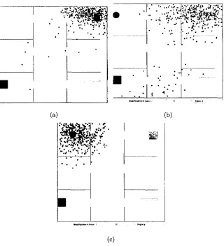
Fig. 4.3 shows localization process in the simulation environment with an obstacle.
Fig. 4.3 (a) shows the beginning of the localization process, where the particles are
not generated yet. In Fig. 4.3 (b) particles are generated based on sensor information.
Fig. 4.3 (c) shows the time that the robot is localized. In Fig. 4.3 (d) robot is being
kidnapped, and Fig. 4.3 (e) shows that robot has recovered from kidnapping problem.
In Tables 4.1, 4.2 and Figs. 4.4 and 4.5 there is a comparison of performance
?Sfi
£1
?tf
• . • • • • • - . ' • •m
:
, * .«.**
* * • *
M M M. i
^
3
..-•
• ' ir
SP
& *
.'--.
• •, r
* : > » • '
^
(c) (d)
(e)
(a)
.?&.?
p
...-. •..*-\. '. :*:
# & '
••' * i
•X-V
" • • • { ' •
^ ' ^ « ? . . ^ .
>1:
•vts
*-•Sv; •: -:.-.
.<;.J
•.AW :'"-7
3&
-(b)
• • • - i S S * # ' ^-: * ' * ,
(e)
Table 4.1: Comparison of performance of the proposed method and traditional MCL, for kidnapping problem in simulation environment without ob-stacle.
Number of Particles 500
1000 1500 2000 2500
Error rate for proposed method (%) 60±14
60±14 52±14 40±14 52±14
Error rate for MCL (%) 100±0
90±8 100±0 80±11 72±12
Table 4.2: Comparison of performance of the proposed method and traditional MCL, for kidnapping problem in simulation environment with obstacle.
Number of Particles 500
1000 1500 2000 2500
Error rate for proposed method (%) 40±14
30±13 32±13 40±14 20±11
Error rate for MCL (%) 80±11 70±13 60±13 62±10 46±14 1.0
o.8 ^
0.6
0.4
0.2
0.0
500 1000 1500 2000 2500
Number of particles
1.0
0.8 -\
0.6
0.4 |
0.2
0.0
MCL with different initialization and resampling
0 500 1000 1500 2000 2500
Number of particles
Figure 4.5: Simulation environment with obstacle.
environment with and without an obstacle in the environment. It shows the Error
rate, which is measured in percentage of time averaged over 50 independent runs,
during which the robot lost track of its position for different number of samples. In
this case, Error rate describes the percentage of lost positions. The results of the
experiments when there is an obstacle in the environment is better since presence
of the obstacle helps the robot to localize itself and removes the symmetry of the
environment.
As it is seen in Tables 4.1 Error rate for MCL in simulation environment without
obstacle when using 2500 particles is 72% which is even higher than using only 500
number of particles in the proposed method. In Table 4.2 also we can see the higher
probability of localization by comparing the Error rates in these two methods in
simulation environment with obstacle. The Error rate when using 2500 particles is
46% in regular MCL which is more than Error rate of 40% when using the proposed
method. In same table, when using 500 particles for the localization process, the
Error rate for the proposed method is 40% and the Error rate for regular MCL is
80%. Using the proposed method we run the program for 50 times and 20 times out
total runs of 50 were not successful. In same table when using 2500 particles, we see
that the Error rate for the proposed method has decreased to 20% and for regular
MCL is decreased to 46%, which indicates 10 unsuccessful results for the proposed
method using 2500 particles and 24 unsuccessful runs for MCL respectively.
4.2.2 Experiments Using Real Robot
We performed two sets of experiments in two different environments in order to make
sure that the proposed method works well in any type of environment. For each real
environment we run regular MCL 50 times for different number of particles and then
we run the proposed method 50 times for different number of particles as well in order
to compare the results of the number of successful localization times. In each set of
experiments, we use different number of particles for localization, since the number of
particles to be used for a specific localization problem is not denned. Therefore, we
performed experiments with different number of particles for each environment and
then we can compare the results.
Figure 4.6: Localization environment without obstacle.
Figure 4.7: NXT calculates its distance to the wall.
to localize itself. In Fig. 4.7, the first time robot gets to the wall and the value of
ultrasonic sensor is less than 20, robot turns 90 degrees and particles are generated,
but after that each time when the value of ultrasonic sensor is less than 20 it rotates
135 degrees.
Figs. 4.8 and 4.9 show the second environment with one obstacle, which is located
in the location (100,300) with size (100,100). When the robot gets to the obstacle, the
weight of the particles in that area will be higher. Generally by an obstacle we mean
something recognizable by the robot which helps it to localize itself. In most cases
they use objects since the robots which are used have vision and they can recognize
different objects by taking pictures and that helps them to localize themselves. Since
NXT provides light sensor which recognizes different colors from each other, we use
color tapes as obstacle, therefore when robot gets to the colored tape it will recognize
it by the value of light sensor and the weight of the particles in that area will be
higher.
Fig. 4.8 (a), (b) show the beginning part of the localization, where there is no
particle generated yet. We put the mobile robot in the experimental environment
(a)
. » . " • ,
• * •
£.V
•. ' "•
; . . v
' »'>Y
Hew P o i U u i <M I1W RalKrt { j 1
^ * • « !
% • ;
• < • % • «
. < ,
. : 1 / . f O
-T^-.r
i »nn if nop
(c) (d)
"^'TffWJMI
"•I«"•'*•. .v
vm
mPosiiztnoMtaRaM
(c) (d)
![Figure 2.1: Probabilistic generation of robot kinematic; (a) A path of moving for-ward; (b) A path of more complicated motion command [25]](https://thumb-us.123doks.com/thumbv2/123dok_us/1455604.1178353/26.600.198.443.213.307/figure-probabilistic-generation-kinematic-moving-complicated-motion-command.webp)