University of Tennessee, Knoxville
Trace: Tennessee Research and Creative
Exchange
Masters Theses Graduate School
12-2011
Capture-recapture of white-tailed deer using DNA
sampling from fecal pellet-groups
Matthew James Goode [email protected]
This Thesis is brought to you for free and open access by the Graduate School at Trace: Tennessee Research and Creative Exchange. It has been accepted for inclusion in Masters Theses by an authorized administrator of Trace: Tennessee Research and Creative Exchange. For more information, please [email protected].
Recommended Citation
Goode, Matthew James, "Capture-recapture of white-tailed deer using DNA sampling from fecal pellet-groups. " Master's Thesis, University of Tennessee, 2011.
To the Graduate Council:
I am submitting herewith a thesis written by Matthew James Goode entitled "Capture-recapture of white-tailed deer using DNA sampling from fecal pellet-groups." I have examined the final electronic copy of this thesis for form and content and recommend that it be accepted in partial fulfillment of the
requirements for the degree of Master of Science, with a major in Wildlife and Fisheries Science.
Lisa I. Muller, Major Professor We have read this thesis and recommend its acceptance:
Craig A. Harper, Joseph D. Clark, Frank T. van Manen
Accepted for the Council: Carolyn R. Hodges Vice Provost and Dean of the Graduate School (Original signatures are on file with official student records.)
CAPTURE-RECAPTURE OF WHITE-TAILED DEER USING DNA SAMPLING FROM FECAL PELLET-GROUPS
A Thesis Presented for the Master of Science Degree
The University of Tennessee, Knoxville
Matthew James Goode December 2011
ii
ACKNOWLEDGMENTS
First, I would like to thank my advisor, Dr. Lisa Muller for giving me the opportunity to be entrusted with this project. Her guidance, patience, and ability to see the positive in any situation was vital in the completion of this project. I am blessed to consider her a mentor and a friend. I am also thankful for the time, patience, and understanding of my committee members, Dr. Craig Harper (who gave me many learning opportunities outside the scope of my own project and made me feel as much a part of his lab as my own), Dr. Joe Clark and Frank T. van Manen (who both gave great insight into the fundamental core of this project). Without any of you, I would have been lost.
Without the financial and logistical support of many entities this project would have never been possible. Rick McWhite, the natural resource manager at Arnold Engineering and Development Center (AEDC) was instrumental in setting up the project and was a great asset throughout. Wes Winton, TWRA manager of AEDC WMA was extremely gracious with his time and resources. Mike Black and Susan Finger helped tremendously with logistical issues and GIS problems. The University of Tennessee Institute of Agriculture and Natural Resources Innovation Fund, Department of Forestry, Wildlife and Fisheries (FWF), and U.S. Fish and Wildlife Service provided funding for the project..
I am indebted to the eager, hard-working, and diligent technicians (Shane McKenzie, Marcus Mustin, Sandra Nash, and Ashley Unger), who endured cold weather, rain, machinegun fire (blanks), mortar shells (simulated), and constant questions about if their job really was to go pick up deer scat in the woods. You made the field season truly enjoyable. To all my fellow FWF grad students, thank you for making my time here not only one of the best learning experiences of my life, but one of the most enjoyable as well. Thanks specifically to Jared Beaver and Seth Basinger who took time out of their lives and projects to help in data collection and overall support. I would also like to thank the staff of FWF for their support, especially Heather Inman and Mirian Wright. Whether it was travel arrangements or tricky package problems they always steered me in the right direction when I had no idea where to go.
iii
I am grateful for all the previous opportunities (jobs) and experiences given to me in this field, which have led me to where I am now. The leadership and wisdom shown to me has been extremely valuable during my time at UT. And of course, I would like to thank my family for all of their support. Even though it took a lot longer than expected and they weren’t quite sure exactly what I was doing, they always found ways to support and motivate me.
iv
ABSTRACT
Reliable density estimates of game and keystone species such as white-tailed deer (Odocoileus virginianus) are desirable to set proper management strategies and for evaluating those strategies over time. However, traditional methods for estimating white-tailed deer density have been inhibited by behavior, densely forested areas that can hamper observation (detection), and invalid techniques of estimating effective trapping area. I wanted to evaluate a noninvasive method of mark-recapture estimation using DNA extracted from fecal pellets as the individual marker and for gender determination, coupled with a spatial detection function to estimate density (Spatially Explicit Capture-Recapture, SECR). I collected pellet groups from 11 to 22 January 2010 at randomly selected sites within a 1-km2 area located on Arnold Air Force Base in Coffee and Franklin counties, Tennessee. I searched 702 plots (10–m radius), collecting 352 pellet-group samples on 197 of the plots. I sent samples to Wildlife Genetics International (Nelson, British Columbia) for genetic analysis. One gender and 6 microsatellite markers with heterozygosity >0.80 were selected for genotyping individuals. Fifteen samples (4%) were not suitable for analysis, 2 (1%) showed evidence of >2 alleles per marker (mixture of DNA), and 114 (32%) failed to provide genotypes during testing. I assigned individual identity and gender to 223 (63%) of the samples which consisted of 39 individuals (18M:21F). I used Program DENSITY (SECR) to fit a model of the detection process to estimate density unbiased by edge effects and incomplete detection. Time of sampling had the largest effect on capture probabilities.
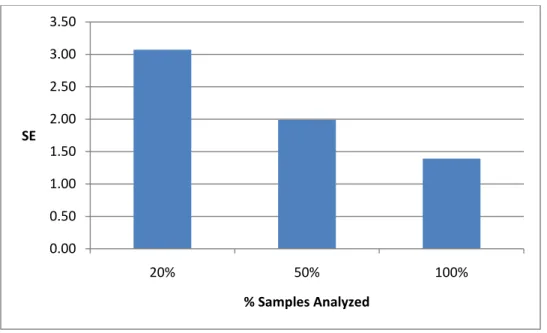
Calculated total deer density was 6.2 (SE = 1.39) deer/km2. Buck to doe ratio was 1:1.75 based on density by gender (2.3 (SE = 0.85) bucks; 4.08 (SE = 1.10) does). I also evaluated whether fewer samples could be used to estimate density with similar measures of precision. Standard error increased from 1.39 for total sample analysis to 1.99 when I evaluated 50% of total
v
samples, and 3.09 when I evaluated 20% of samples. I found DNA sampling from pellet groups provided deer density and sex ratio estimates useful for deer management decisions and reduces the risk of overestimating deer density, common in traditional methods.
KEY WORDS: capture-recapture,density, DNA, fecal pellets,mark-recapture, microsatellites,
vi
TABLE OF CONTENTS
I. INTRODUCTION ... 1
BACKGROUND ... 1
TECHNIQUES FOR ESTIMATING DEER POPULATIONS ... 4
PELLET GROUP COUNTS ... 7
GENETIC SAMPLING FOR DENSITY ESTIMATION ... 10
SPATIALLY EXPLICIT CAPTURE-RECAPTURE ... 12
JUSTIFICATION ... 14
OBJECTIVES ... 15
II. STUDY AREA ... 15
STUDY AREA ... 15 III. METHODS ... 16 FIELD PROCEDURES ... 16 GENOTYPING ... 18 DENSITY ESTIMATION ... 20 IV. RESULTS ... 22 FIELD SAMPLING ... 22 GENOTYPING ... 22 DENSITY ESTIMATION ... 23 V. DISCUSSION ... 24
VI. MANAGEMENT IMPLICATIONS... 29
LITERATURE CITED ... 30
APPENDICES ... 47
APPENDIX A: TABLES ... 48
APPENDIX B: FIGURES ... 54
vii
LIST OF TABLES
Table 1. Microsatellite marker variability, observed and expected heterozygosity, and
observed number of alleles of white-tailed deer on Arnold Air Force Base, Tennessee, USA, 2010. The first 6 markers, and a gender marker, were run on every sample for the purpose of individual identification……….46 Table 2. Number of plots searched, number of plots with at least one sample found, total number
of samples for capture events, and average number of samples for white-tailed deer pellet groups, at Arnold Air Force Base, Coffee and Franklin counties, Tennessee, USA, January 2010. A rain event occurred between sampling period 3 and 4 (17 January, 2010)………47 Table 3. Model selection and density (D) estimates of white-tailed deer population on Arnold
Air Force Base, Tennessee, USA, 2010. Half-normal (HN) detection function was evaluated. The capture probability parameter g0 was modeled as a function of linear time (TL), time before and after rain event (17 January 2010; that occurred between sampling periods 3 and 4 (T3-4)), as a mixture for individual heterogeneity (H2) and as a constant (.). Spatial scale (S) was modeled as H2 and as a constant………...48 Table 4. Model selection and density (D) estimates of white-tailed deer population on Arnold
Air Force Base, Coffee and Franklin counties, Tennessee, USA, January 2010, by gender for the determination of sex ratio. HN detection function was evaluated and capture probability parameter g0 was modeled as a function of linear time (TL), time before and after rain event (17 January 2010; that occurred between sampling periods 3 and 4 (T3-4)), as a mixture for individual heterogeneity (H2) and as a constant (.). Spatial scale (S) was modeled as (H2) and as a constant………49 Table 5. Model-averaged density (D) estimates, SE, Variance, and Lower and Upper 95%
confidence intervals for 100% and sub-samples (50% and 20% of total samples used) of white-tailed deer population on Arnold Air Force Base, Coffee and Franklin counties, Tennessee, USA, January 2010. HN detection function was evaluated and capture probability parameter g0 was modeled as a function of linear time (TL), time before and after rain event (17 January 2010; that occurred between sampling periods 3 and 4 (T3-4)), as a mixture for individual heterogeneity (H2) and as a constant (.). Spatial scale (S) was modeled as (H2) and as a constant………....50
viii
LIST OF FIGURES
Figure 1. Study area map of Arnold Air Force Base, Coffee and Franklin Counties Tennessee, USA for collection of white- tailed deer pellet groups, January 2010………...52 Figure 2. Model-averaged Standard Error (SE) for 20%, 50% and 100% of samples collected
1
I. INTRODUCTION
Background
At the time of European settlement white-tailed deer (Odocoileus virginianus) were abundant and widespread throughout the eastern United States (McCabe and McCabe 1984). White-tailed deer were an important species for both Native Americans and initial settlers who harvested white-tailed deer for food, trade and cultural significance. During European settlement populations declined and there was a 35-50% reduction of an initial estimated 23–34 million white-tailed deer (McCabe and McCabe 1984). However, this decline did not decimate the population possibly because of cultural land management practices (burning) and meteorological events (hurricanes, tornadoes, and lightning) that provided early succession vegetation and edge and favored deer (McCabe and McCabe 1984).
During the 19th century (1800–1865) white-tailed deer populations increased modestly but likely did not reach pre-settlement populations (McCabe and McCabe 1984). However, the increase was only seen in unexplored lands as settlers began to enter the continental interior and traditional Native American influence on the land ceased. As settlers moved west, new
populations of deer were discovered. Land that was abandoned in the east began to recover from overexploitation which attracted and supported white-tailed deer populations. This change in deer habitat use gave the illusion that populations were increasing and led to market and
subsistence hunting in what is known as the exploitation era (1850–1900; McCabe and McCabe 1984).
Many white-tailed deer populations were virtually extirpated late in the 19th century because of human exploitation (Noble 1966, Ellsworth et al. 1994). White-tailed deer were used
2
extensively for food, clothing, a growing market developed for hides, venison, and other carcass products (e.g., antlers, hair, tallow). The white-tailed deer was also perceived as a pest to crop production. Market hunting reached its climax after the Civil War with the advent of repeating rifles and expansion of the railroad system (McCabe and McCabe 1984).
By 1920, white-tailed deer populations reached a historical low and remained at low levels until restoration efforts were initiated by federal and state wildlife agencies after World War II (Ellsworth et al. 1994). Federal agencies initiated restoration efforts that encompassed protective legislation, habitat management, and restocking programs (reviewed in McCabe and McCabe 1984). Approximately 8,000 deer were restocked in Alabama, Florida, Georgia, and South Carolina from source populations native to and outside the region (reviewed in McCabe and McCabe 1984). Whereas the North American white-tailed deer population was estimated at 500,000 individuals in the early 1900s it currently exceeds 20 million individuals (Cook and Daggett 1995, Hubbard et al. 2000).
White-tailed deer are widely distributed throughout North America extending from the Yukon and Northwest Territories across the southern provinces of Canada and south into Central and South America. White-tailed deer are present throughout the contiguous United States (Miller et al. 2003). During the last 20 years abundant white-tailed deer populations have caused a rise in crop and property damage and number of deer-vehicle collisions (DVCs; Conover et al. 1995, Romin and Bissonette 1996). Annually, >1 million DVCs occur in the United States, resulting in >$1 billion in property damage and personal injury (Conover et al. 1995, Ng et al. 2008). Four to 5% of DVCs result in human injury and there are >200 human fatalities annually (Hansen 1983, Conover et al. 1995, Biggs et al 2004). From 1981 to 1991, nationwide estimates
3
of vehicular damage have averaged approximately $2,000 per DVC (Romin and Bissonette 1996, Biggs et al. 2004).
High deer density influences the structure and composition of forest understory (Tilghman 1989, Rossell 2005). Elevated deer density and chronic over-browsing limits
availability of food and cover for many wildlife species in forested areas (Casey and Hein 1983, deCalesta 1994) and impacts both faunal and floral species diversity (Anderson 1993, Rossell 2005, Webster 2005, Rossell et al. 2007). Overbrowsing by deer also can negatively affect the overall health of the deer populations (Johnson et al. 1995). Overabundant white-tailed deer herds can create alternate stable states (stable ecological succession stage other than predicted) in ecological communities (Stromayer and Warren 1997). White-tailed deer overabundance has become, and likely will remain one of the most intricate issues concerning wildlife managers (Warren 1997).
White-tailed deer are also the most popular game animals in the U.S. The number of days spent deer hunting and the associated expenditure exceed that from all other species combined (U.S. Fish and Wildlife Service et al. 2007). An estimated 10.7 million hunters pursued big game in 2006 of which 10.1 million hunters spent 132 million days pursuing deer (Odocoileus spp.; U.S. Fish and Wildlife Service et al. 2007). Deer hunters make up 81% of all hunters ≥16 years. Big game hunters averaged about 15 days of hunting and spent $435 per hunter.
Equipment and trip expenditures for big game hunting totaled $11.8 billion (U.S. Fish and Wildlife Service et al. 2007).
4
Techniques for Estimating Deer Populations
White-tailed deer affect the ecosystem, economy, and safety of highways, so it is desirable to have accurate population and sex ratio estimates to facilitate management. Reliable population estimates are important for management protocols and conservation policies for any wildlife species, but are particularly important for management of threatened, endangered, or game species (Wemmer 1997, Cederlund et al. 1998, Koenen et al. 2002, Valière et al. 2007). Detecting changes in local populations is important in evaluating the effectiveness and efficiency of management protocols of harvested species (Gibbs 2000).
Many techniques have been developed to estimate population abundance and sex ratio of white-tailed deer including, aerial surveys, hunter observations, spotlight counts,
infrared-triggered camera surveys, forward-looking infrared surveys, pellet-group counts, removal methods, distance sampling, and capture-recapture (Bennett et al. 1940, Rice and Harder 1977, McCullough 1982, Wiggers and Beckerman 1993, Jacobson et al. 1997, Belant and Seamans 2000, Koenen et al. 2002). However, many of these techniques only indicate relative changes in population size over time and do not provide accurate abundance, density estimates or sex ratios. The changes in population size determined by these techniques may not accurately represent population growth or decline, because many are unable to account for natural yearly fluctuations in populations, which may result in inappropriate management of populations (Gibbs 1998).
Adult sex ratio affects population growth and therefore harvest strategies (Hamilton et al. 1995). Many traditional population estimation techniques are unable to directly measure sex ratio and those that can assume similar detection and social behavior between genders (Downing et al. 1997, Jacobson et al. 1997, Mccoy et al. 2011). Baiting can lead to dominant individuals
5
controlling the resource not allowing subordinate individuals to be detected (or be detected at a lower rate) and males and females may behave differently in response to road surveys. Grouping of individuals (e.g., bachelor groups, does with fawns) and timing of year can also influence counts. Techniques that estimate sex ratio based on physical characteristics (antlers) to distinguish unique individuals are limited to specific times of the year (McKinley et al. 2006).
Population estimates using well-established statistical techniques that account for imperfect detectability (the probability of detection is less than 1.0) are preferred to uncorrected counts (White 2005, Royle and Young 2008). Although statistical techniques are preferred, uncorrected index counts converted to density are still commonly used for species in remote areas, are difficult to capture or exhibit reclusive tendencies (Harris et al. 2010).
Dense forests in the southeastern United States hamper density estimation for ungulates (Koster and Hart 1988, van Vliet et al. 2008). For example, aerial and ground surveys may not be reliable because dense canopies and understory restrict surveys to easily accessible roads and open areas (Anderson 2001, Brinkman et al. 2011). Different techniques can lead to drastically different estimates. Mandujano and Gallina (1995) used 3 different techniques (track count, pellet-group count, and direct counts on transects) for the same population of white-tailed deer and reported wide ranging density estimates (1.6 to 27.6 deer/km2). Restriction of surveys to easily accessible areas may also affect sex ratio estimates.
Capture-recapture techniques can provide accurate and robust results when assumptions associated with the design can be met (Schwarz and Seber 1999, Williams et al. 2002). Capture-recapture experiments using live captures or remote cameras have been used to estimate white-tailed deer populations (Rice and Harder 1977, Roberts et al. 2006). However, many studies with deer rely on baiting which may violate equal detectability and may lead to unmodeled
6
heterogeneity (Cutler and Swann 1999, Roberts et al. 2006). Also, techniques that require live capture and tagging of ungulates are labor intensive, costly, risk animal mortality generally have a limited spatial scope and often result in population estimates with low precision and accuracy because of low sample sizes (Pollock et al. 1990, Patterson et al. 2003, Brinkman et al. 2011). These techniques generally can only estimate population abundance because of problems associated with trapping area.
Traditional density estimates are calculated by dividing abundance estimates by the effective trapping area (Dice 1938, Efford 2004). However, many of these estimates are biased because of ineffective methods of calculating effective trapping area (e.g., edge effect because of temporary immigration or emigration or behavioral response to traps; Efford 2004, Lancia et al. 2005, Royle and Young 2008). Dice (1938) recommended adding a buffer with a width of a home-range radius to the exterior boundaries of the trapping area to determine the effective trapping area. However, estimates of home range size, and thus the buffer width, can be biased by ranges at the edge of the trapping area. Individuals whose core area only occupies a small portion of the trapping area because of temporary movements in and out of the trapping area will reduce capture probabilities and therefore inflate the density estimate and poorly estimate
effective trapping area (Boulanger and McLellan 2001, Royle and Young 2008). Other methods have since been developed to estimate buffer width from capture-recapture data but they have not been broadly applied (Otis et al. 1978, Gurnell and Gipps 1989, Parmenter et al. 2003). Estimation of effective trapping area is difficult and is usually determined ad hoc resulting in questionable density estimates (Efford 2004). Trap response can bias population abundace estimates high or low. If the trap response is positive (e.g., bait) then density estimates will be
7
biased high and if the trap response is negative (e.g., stress from capture) then density estimates will be biased low (Nichols et al. 1984).
Many techniques used to index populations assume detection of the population will remain constant in every year and that changes in survey numbers represent changes in actual population size. Currently the most reliable techniques used to estimate white-tailed deer populations rely on assumptions that are often overlooked. Techniques are still needed to
accurately estimate density and sex ratios without the use of an arbitrarily defined area, have the ability to account for changes over time, and do not influence behavior. However, this is often not feasible resulting in expensive monitoring programs that lack statistical power to identify population trends (Gibbs 1998). It may be possible to combine techniques to add statistical power and utilize the spatial distribution of recapture (e.g., spatially explicit capture-recapture using genetic sampling from pellet groups).
Pellet Group Counts
Bennet et al. (1940) first described systematic pellet-group counts of white-tailed deer populations in Pennsylvania. Pellet-group sampling is used to estimate population abundance and habit use of big game species (Neff 1968, Rogers 1958). Indices derived from fecal pellet counts are commonly used to investigate and monitor ungulate populations in forested
landscapes (Neff 1968, Kirchhoff 1994, Patterson and Power 2002, Forsyth et al. 2007, van Vliet et al. 2008). Counts can be used to estimate yearly population trends or be divided by pellet-groups/deer/day to estimate deer numbers and deer-days of habitat use. Accuracy and precision of abundance estimates derived using the pellet-group technique depend on many variables such as pellet group density, pellet group distribution, size of the area to be sampled, defecation rate,
8
observation bias and persistence of pellet-groups in the system (Rogers et al. 1958, Van Etten and Bennett 1965).
Pellet-group sampling is more efficient in areas of high pellet-group density. If possible, winter ranges and other concentrated areas should be chosen for herd census or trend studies. Pellet-group density may vary between south and north slopes and different vegetation types (reviewed in Neff 1968). Distribution of pellet-groups may be random, regular, or clumped. However, pellet-groups are found more often in a clustered arrangement. Therefore, preliminary surveys are necessary for a pellet-group sampling program because they provide estimates of mean pellet-group density and distribution (Neff 1968).
An inverse relationship exists between the percentage of an area that needs to be sampled for pellet groups and the size of the sampling area to attain desired confidence limits. Thus, as sampling area increases the percent of the area that needs to be searched decreases to maintain a constant precision. If pellet-group density remains the same for the whole area, the precision of the estimate of mean pellet-group density remains the same on a large as on a small area. However, if deer use is highly variable over a large area a larger sample size may be required to maintain similar confidence limits (Neff 1968).
Pellet-group data can be used to describe population trends without considering
defecation rate, if defecation rates are similar across all years. However, to calculate total deer-day use, or total number of animals present, defecation rates per deer-day are needed. Some factors believed to affect defecation rates are season, range condition, feed intake, moisture content in forage and percentage of fawns in the winter herd (Longhurst 1954, Rogers et al 1958, Smith 1964). Penned deer in Michigan had a mean of 12 pellet-groups/deer/day between February and March (Eberhardt and Van Etten 1956) and 13.2 pellet-groups/deer/day between January and
9
April (reviewed in Neff 1968). Rollins et al. (1984) found an average of 19.6 pellet-groups/deer/day in penned deer in Texas. However, much higher rates were found in free-ranging female white-tailed deer in Minnesota (Rogers 1987) and Georgia (Sawyer et al. 1990), with 22.3–51.9 and 23.5–31.3 pellet-groups/deer/day, respectively.
Observer bias occurs when pellet-groups are miscounted. Miscounts can be from human error caused by fatigue, boredom, vision, and experience, or because of ground cover, and size and shape of plots. Pellet groups are more likely missed when sampling larger concentric circular plots compared to smaller plots and belt transects compared to circular plots (Neff 1968).
Loss of pellet groups from erosion is considered unimportant unless ground cover is sparse. Even on slopes of 60–80%, litter and vegetation held pellet-groups (Neff 1968). Van Etten and Bennet (1965) found some pellet-groups still appeared fresh even after 2 years and some persisted beyond 5 years. The main reasons for pellet-group loss were washing by rain and concealment by litter. However, loss was not large enough to cause problems for annual or semi-annual pellet-group counts (Van Etten and Bennet 1965). Harestad and Bunnell (1987) found pellet-groups deteriorated much faster in moist forested conditions compared with dry
conditions. Location and climate cause variability in persistence and deterioration rates of pellet-groups. Considerable deterioration of pellet-groups can be attributed to insects (Neff 1968).
Although fecal pellet counts have been commonly used to estimate ungulate populations, they can be imprecise, inaccurate, and unreliable (Fuller 1991, Campbell et al 2004) because of variability in persistence of pellet groups (e.g., seasonal and weather effects on pellet
degradation), variability in defecation rates, variability in detectability of pellets in various vegetation types (observation errors). Statistical procedures used to estimate populations from
10
fecal counts lack empirical data and are rarely evaluated over time (Brinkman et al. 2011). Furthermore, few studies have evaluated the relationship between pellet-group counts and deer density (Forsyth 2007). However, extraction of nuclear DNA from fecal pellets of white-tailed deer for individual genetic profiles and gender determination has recently become possible (D. L. Paetkau, Wildlife Genetics International (WGI), unpublished data).
Genetic Sampling for Density Estimation
Traditional capture-recapture techniques use physical markers (e.g. eartag, tattoo, branding) but genetic sampling can be used to obtain capture-recapture data without handling, capturing, or even observing individuals by using genetic material to mark individuals (Waits and Paetkau 2005). Use of genetic sampling ensures tag permanency, decreases intrusiveness, and can be effective to increase capture probabilities, reduce capture bias, and shorten the
sampling period (Taberlet et al. 1999, Woods et al. 1999, Mills et al. 2000). Genetic sampling is a relatively new technique that provides great potential for research and management
applications in wildlife biology (Taberlet et al. 1997, Woods et al. 1999, Mowat and Strobeck 2000), especially for capture-recapture studies. Scat and hair are the most common sources of DNA obtained for genetic sampling (Miller et al. 2005).
Initial research efforts using genetic sampling were based on tissue samples to determine abundance of humpback whales (Megapteranovaeangliae) in the North Atlantic Ocean (Palsbøll et al. 1997) and hair samples to determine abundance of brown bears (Ursus arctos) in British Columbia (Mowat and Strobeck 2000, Poole et al. 2001). Hair snares have been used to collect genetic samples from the hairy-nosed wombat (Lasiorhinus krefftii, Banks et al. 2003), marten (Martes americansus, Mowat and Paetkau 2002, Williams et al. 2009), San Joaquin kit foxes
11
(Vulpes macrotis mutica, Bremner-Harrison et al. 2006) and swift foxes (Vulpes velox, Bremner-Harrison et al. 2006), wolverine (Gulo gulo, Magoun et al. 2011), grizzly bear (Ursus arctos; Boulanger et al. 2004, Kendall et al. 2008), and black bear (Ursus americanus; Settlage et al. 2008, Clark et al. 2010). Efforts to monitor ungulate populations using genetic sampling from hair are scarce but included a study on white-tailed-deer (Belant et al. 2007)
Population estimates using NGS from feces was first conducted successfully for coyote (Canis latrans, Kohn et al. 1999) and later on mountain lion (Puma concolor; Ernest et al. 2000), grey wolves (Canis lupus, Creel et al. 2003), African forest elephant (Loxodonta cyclotis, Eggert et al. 2003), European badger (Meles meles, Wilson et al. 2003), wolverine (Flagstad et al. 2004, Hedmark et al 2004) and brown bears (Bellemain et al. 2005). Use of genetic material obtained from pellet groups has been conducted in red deer (Cervus elaphus; Valière et al. 2007), red duiker (Cephalophus natalensis) and yellow-backed duikers (Cephalophus sylvicultor; van Vliet et al. 2008), Ethiopian walia ibex (Capra walie;Gebremedhin et al. 2009), argali (Ovis ammon; Harris et al. 2010), and Sitka black-tailed deer (Odocoileus hemionus sitkensis; Brinkman et al. 2011). However to our knowledge, no one has used fecal DNA to estimate abundance of free-ranging white-tailed deer.
Fecal pellets contain cells shed off the intestinal lining and DNA extracted from those cells can be used as an individual marker. Thus, this technique can potentially provide abundant samples for capture-recapture studies (Maudet et al. 2004) for low cost (Foran et al. 1997, Brinkman et al. 2011), and without animal capture or disturbance (Belant 2003, Belant et al. 2005). However, diet may affect analysis. High-quality and low-fiber diets during spring (buds and young shoots) increase the digestive process while reducing contact time and abrasion of the intestinal walls. Conversely, summer and winter diets (twigs, dry grasses, and lichens) cause
12
more abrasions and remain in the digestive track longer allowing for greater amounts of genetic material to accumulate on fecal pellets (Mauedet et al. 2004). The amount of DNA material available for genetic analysis on fecal pellets is very small and varies among samples, which can lead to polymerase chain reaction (PCR) amplification errors (Gerloff 1995) and the generation of false alleles or allelic dropout (Taberlet et al. 1996). Smaller allele lengths have a greater amplification success and fewer allelic dropouts than longer alleles (Buchan 2005). Wet weather conditions that dissolve or wash genetic material from pellet groups and extended times of exposure can cause high failure rates in DNA analysis (Murphy et al. 2007). With Sitka black-tailed deer Brinkman et al. (2009a) found that only 22% of fecal samples exposed to
environmental factors for 7 days were successful for microsatellite analysis. None were successful after 14 days of exposure compared with 80% success rate for samples left in a
controlled environment up to 28 days. Contamination from ingested tissue and or hair could also lead to genotyping errors (Wasser et al. 1997).
Because pellet groups are abundant and can remain in the environment for long periods of time, the large number of samples collected can affect the processing capacity of genetic labs (Harestad and Bunnell 1987, Brinkman et al. 2011). Therefore, stratifying samples based on likelihood of success before analysis may be beneficial to reducing cost. Also, defecation rates can vary among locations and seasons and should be considered in the sampling scheme. Differences in defecation rates can influence the number of samples needed for analysis.
Spatially Explicit Capture-Recapture
The spatial relationship within capture-recapture data is usually neglected or ignored during analysis (Efford et al. 2009). Efford (2004) incorporated trap (detector) locations with
13
capture probabilities, for a spatially explicit capture-recapture method (SECR; Borchers and Efford 2008). Efford (2004) used a 2-parameter spatial detection function to represent the capture process and fit a linear model. Animal range centers within the study area are directly correlated to the overall density of that area. Each animal is assumed to occupy a range center at an unknown location and each trap (detector) is set at a known location. Therefore, the
probability of capture is a declining function of distance between the range center and the trap, similar to the detection function in distance analysis (reviewed in Efford 2004). Neither the individual range center nor the complete ranges of movement coordinates are fully observed but can be predicted (Royle and Young 2008). Efford et al. (2009) constructed a likelihood-based model for capture histories that include the location of detection. The model includes a capture submodel with parameter g0 and a distribution submodel with parameter σ.
The capture submodel gives the probability of detecting an individual in a particular trap based on the location of its range center and can account for different types of detectors (e.g. proximity, multi-catch, single-catch). Initially, the method was designed to only allow for each trap to capture 1 animal (single-catch). However, proximity detectors allow for movements of animals after detection (not limiting an animal to only be captured once during an occasion) and multiple animals can be captured at the same trap. This type of detector is useful for passive sampling techniques, such as with DNA sampling and camera traps (Royle et al. 2011). Multi-catch detectors are similar to proximity detectors by allowing multiple individuals to be captured at one trap but individuals detected in one trap cannot be detected in another for the same
occasion (e.g. mist nests and pit fall traps). The distribution submodel (σ) accounts for the distribution of range centers in the sampling area and the intensity of those range centers within
14
the sampling area is equivalent to density (Efford et al. 2009). Covariates, mixture models, differences in density between sites and times may be included in the analysis. This type of analysis produces density estimates unbiased by edge effects and incomplete detection (Efford et al. 2004).
Statistical software packages are available for analyzing spatially explicit capture-recapture data. Program DENSITY (http://www.otago.ac.nz/density/) and SECR in Program R (http://www.otago.ac.nz/density/SECRinR.html) are available for free download and serve as an interface to incorporate spatially explicit capture-recapture data from a variety of detector types.
Justification
Information on population abundance is useful when managing wildlife species especially those that are harvested and have the potential to become overabundant. Reliable estimates of white-tailed deer populations are important for appropriate management and harvest regulations. At Arnold Air Force Base (AAFB), Coffee and Franklin counties, Tennessee, white-tailed deer impact forested systems particularly threatened and endangered flora and fauna species, and cause deer-vehicle collisions. However, they are an important natural resource for deer hunting. Thus, management goals and objectives set by AAFB would benefit from accurate estimates of deer density and sex ratio to minimize impacts from deer-vehicle collisions and effect on threatened and endangered species, while maximizing hunter satisfaction. Techniques used to estimate white-tailed deer populations and determine sex ratios are impaired by logistical problems and biases that culminate in loss of precision and accuracy. Spatially explicit capture-recapture methods using genetic sampling for monitoring white-tailed deer herds may overcome these problems.
15
Objectives
The overall goal of my study was to evaluate genetic sampling from pellet groups for SECR in white-tailed deer. The specific objectives of my study were to:
1) Evaluate the potential of genetic sampling from scat (pellet groups) to estimate white-tailed deer density.
2) Evaluate the potential of genetic sampling from scat (pellet groups) to estimate the sex ratio of white-tailed deer.
II. STUDY AREA
Study Area
I conducted this study at Arnold Air Force Base (AAFB), located in Coffee and Franklin counties, Tennessee (Figure 1). The base was approximately 112 km southeast of Nashville, positioned between the towns of Manchester, Tullahoma, and Winchester, and is within the Duck and Elk River watersheds (United States Department of Defense 2006). The deer population on AAFB was managed jointly by Department of Defense (DoD) and the Tennessee Wildlife Resources Agency (TWRA). A majority of the area on AAFB was open to public hunting and was managed as a Wildlife Management Area (WMA) by TWRA.
Arnold Air Force Base encompassed 15,815 ha. Cultivated loblolly pine (Pinus taeda) plantations or continuous hardwood forest mostly dominated by combinations of southern red oak (Quercus falcata), scarlet oak (Quercus coccinea), post oak (Quercus stellata), black oak (Quercus velutina), white oak (Quercus alba), willow oak (Quercus phellos), water oak (Quercus nigra), and blackjack oak (Quercus marilandica) covered 11,553 ha. The understory
16
included dogwoods (Cornus spp.), maples (Acer spp.), sassafras (Sassafras albidum), sourwood (Oxydendrum arboretum), blueberries (Vaccinium spp.), hickories (Carya spp.), and blackgum (Nyssa sylvatica). Grasslands and early-successional vegetation in utility rights-of-way occupied 898 ha. The remaining 1,895 ha of the installation was occupied by wildlife food plots, buildings and structures, mowed areas, and other open areas (e.g., landfills, roads; United States
Department of Defense 2006).
Field sampling was concentrated within a 100 ha area in Unit 1 of AAFB (Figure 1). The area in Unit 1 consisted of 51.0 ha of hardwood, 38.3 ha of pines and 7.2 ha of fields. The hardwood sections were dominated by post oak (35.7 ha) and southern red oak (15.3 ha). The proportion of vegetation types was similar across all of AAFB.
III. METHODS
Field Procedures
I conducted a pilot study to determine how many plots and samples were needed for a recommended 20% recapture rate (Otis et al. 1978). I searched 20 10-m radius plots for pellet groups within the study area and found 20% of the plots had at least 1 pellet group. I established a 10-m radius from the center of the plot and marked the four cardinal directions with flags (Neff 1968). I visually searched the plots and collected all pellet group samples within the plot. All pellet groups in the plots were removed to avoid resampling of the same pellet group. Assuming deer deposited 10 pellet groups/day (Eberhardt and Van Etten 1956) and based on a density of approximately 8 deer/km2 (J. Beaver, University of Tennessee, unpublished data), I estimated approximately 160 pellet groups/2-day capture event. Therefore I needed approximately 150
17
plots to collect about 32 pellet group samples per sampling occasion. I established 5 sampling occasions and a sampling occasion was defined as a sequential 2-day period and was continuous with no time between occasions. Therefore I needed to collect about 160 pellet-group samples from approximately 750 plots. Five to 6 technicians searched plots over the 100 ha study area.
I generated 150 randomly selected global positioning system (GPS) locations using Arc Map (ESRI® ArcMap 9.3.1, 1999-2009) for each of the 5 sampling occasions (total of 750 GPS locations). A 20-m radius buffer was added around each point to protect against plots
overlapping during individual capture events. Plot designation was the same as for the initial sampling. I collected pellets adjacent to each other within the pellet group. I avoided collecting pellets scattered more than approximately 0.1 m2 from the center of the pellet group to decrease the probability of collecting from more than one individual (Harris et. al 2010). Fresh Latex gloves were used to collect each sample. I recorded GPS location of the plot, date, name of collector and general appearance of the pellets. Samples were rated for quality: a sample coded as 1 was considered fresh and of high quality (still moist, intact, and above litter), 2 represented intermediate quality and freshness (somewhat moist, intact), and 3 represented low quality and older age (dry, easily broken, under liter). I placed fecal pellets in paper bags that were labeled in the field. All pellet groups were removed from plots to avoid resampling if the same area was searched in a later sampling occasion. Samples were allowed to dry at room temperature and desiccant was placed around the paper bags in a storage box to facilitate drying (D. L. Paetkau, Wildlife Genetics International, personal communication).
18
Genotyping
All samples were sent to Wildlife Genetics International (WGI; Nelson, British Columbia, Canada) for genetic analysis. Fecal pellets were analyzed for individual genetic profiles and gender determination. Pellets that were broken open, crushed or clumped together were not analyzed because of the high probability that inhibitory secondary plant compounds compounds within the feces would co-purify with the DNA and thus compromise success rates (Wilson 1997). WGI immersed 1–6 pellets, depending on size and availability, in Qiagen’s ATL digest buffer (Qiagen, Valencia, California, USA) in a test tube and agitated by gentle swirling several times over 1 hour. Pellets were removed from the solution and DNA purification followed methods described in Woods et al. (1999) and Paetkau (2003).
WGI used 21 microsatellite markers routinely used in parentage projects involving white-tailed deer to determine individual identification (BL25, BL42, BM4107, BM6438, BM6506, FCB193, Inra11, OheK, OhemD, OhemH, OhemN, OhemO, OhemP, OhemS, OheQ, OhL, OvirA, Rt5, Rt7, Rt13, and Rt24). WGI excluded markers that amplified weakly from fecal samples, including markers with allele lengths over 200bp. Amplification of DNA from fecal extracts was sensitive to the length of the DNA segment analyzed. After removing markers problematic for success rate (OheK, OheQ, OhL, and Rt13), and sequencing enough samples to have at least 15 animals genotyped at each marker, WGI compared 17 markers for variability, success rate and ability to fit together efficiently in a single sequencer lane (Table 1). WGI selected 6 markers with heterozygosity ≥0.80 (BL42, BM4107, FCB193, OhemS, Rt5, Rt7; Table 1) and added a ZFX/ZFY gender marker alongside the microsatellites.
Samples were stratified by confidence data scores after all had been analyzed at each of the 7 markers. WGI used a combination of objective (peak height) and subjective (appearance)
19
criteria to classify genotype scores. Samples were stratified into 3 groups: those that yielded high-confidence scores for 6 or 7 markers on the first pass, those that yielded high-confidence scores for 3–5 markers, and those that yielded ≤2-locus genotypes. Those that yielded high-confidence scores for 3–5 markers during the first pass were re-analyzed 3 more times at all 7 markers to evaluate run-to-run data reproducibility. For these samples a multilocus consensus genotype was identified for each sample, and each repeat was assigned a value of 0, 0.5 or 1 based on whether 0, 1, or 2 alleles, respectively, matched those in the consensus genotype. These values were averaged across all 4 repeats of all 7 markers to arrive at q,the likelihood that genotype belonged to a unique individual. Samples with q < 0.6 were culled. Samples with q > 0.6 where by the 4 repeats of analysis did not produce at least 2 high-confidence scores (identical to the consensus genotype for a given marker) were subject to further rounds of single-locus analysis to confirm the genotype. Samples with ≤2-locus genotypes were culled. Individual were identified based on their unique, 7-locus genotype.
A major assumption for capture-recapture studies is that individuals are correctly
identified upon recapture. If samples from the same individual are assigned different genotypes, then more individuals will be identified than are actually present in the study area causing error in the density estimate. Also if marker variability is not high enough to uniquely identify individuals, then fewer individuals will be identified than are actually in the study area (Woods et al. 1999, Mills et al. 2000). Therefore, WGI personnel re-analyzed markers that mismatched at 1 or 2 of 7 markers to check for errors. WGI found and corrected errors in 14 samples because of amplification errors at the OhemS and BL42 marker. After correcting for errors there is no reasonable probability that the number of individuals identified in the dataset has been inflated through undetected genotyping error (Kendall et al. 2009).
20
Density Estimation
I used capture histories and capture locations of individuals identified based on their genetic profile to estimate white-tailed deer density using Program DENSITY (version 4.4; http://www.otago.ac.nz/density/, accessed 15 July 2011). Spatially explicit calculation of density involves a detection probability parameter g0 and a spatial scale parameter σ (Efford 2004). Detection was modeled as the half-normal function (Borchers and Efford 2008). Assuming the animals were distributed randomly across the landscape I modeled the number of captured individuals as a Poisson distribution (Borchers and Efford 2008). I used a priori models including individual heterogeneity as a 2-class mixture model that delineated individuals into unobserved sub-groups for both g0 and σ parameters and assumed no behavioral response because pellets were passively collected. I also modeled g0 as a function of time. I considered a linear time trend but also modeled g0 as a function of a rain event that occurred between capture events 3 and 4 (17 January, 2010), which could have affected capture probabilities. I calculated buffer width of ~1500 m by multiplying root-pooled spatial variance (RPSV = 339.1) x 4 as recommended by Efford et al. (2004). I did not use a habitat mask because surrounding the sampling area was considered suitable deer habitat. To compare models I used Akaike’s Information Criterion adjusted for small sample sizes (AICc):
2 ˆ log 2 , 1 c n AIC n K n K where, K is the number of parameters including the intercept and:
2
2 ˆ
ˆ i
21
Models with lower AICc values were considered to have more support and be more
parsimonious (Burnham and Anderson 2002). I compared differences in AICc values (ΔAICc) to evaluate the relative importance of the models; when models had a ΔAICc value of <2, they were considered to have equal support. Model weights (wi,) were calculated as:
1 1 exp 2 1 exp 2 i i R i r w ,
where R is the number of models in the candidate set and r is the first model in the summation (Burnham and Anderson 2002), and were used to compare support allowing us to make inferences about precision over the entire suite of models (Burnham and Anderson 2002). I calculated density using all captures (genders combined) and each gender separately. Density by gender was used to calculate sex ratio.
I also wanted to evaluate if fewer samples could be used to estimate density with similar precision compared with using all samples. To do so, I repeated our analyses based on
subsampling regimes of 50% and 20% of the total pellet groups with individual genotypes. I used the same models and conducted 10 iteration of each subsampling regime, each time selecting a new set of random samples from the full dataset. I again used model averaging to estimate density, standard errors, and variance for each suite of models on each individual run of the iterations. I used 95% confidence intervals to compare density among the full dataset and the 2 subsampling regimes. I calculated mean standard error across the 10 iterations for each
22
IV. RESULTS Field Sampling
I collected pellet groups during 11–22 January 2010. Technicians spent 8–10 hrs/day searching approximately 70 plots during each 2-day sampling occasion. I sampled 703 plots, 197 of which had ≥1 pellet-group sample (28%). I collected 352 pellet-group samples (Table 2). The greatest number of pellet groups found in 1 plot was 8 (0.05%). Overall, 15% of the plots had 1, 8% had 2, and 3% had 3 pellet groups/plot. I searched 4% of the total area (140 10m circular plots per capture event) which yielded an average of 70 samples per capture event. A major rain event occurred on 17 January, between capture events 3 and 4. Mean number of pellet groups/sampling occasion prior to the rain event was 78 and mean number after the rain event was 58.
Genotyping
I used all 352 pellet-group samples for microsatellite analysis. Fifteen samples (4%) were inadequate for analysis because pellets were broken open, crushed, or clumped together. A total of 337 pellet-group samples were used for genetic analysis. Two samples (1%) showed evidence of >2 alleles per marker suggesting a mixture of DNA from 2 individuals, and were not used in the final analysis. One hundred and fourteen samples (34%) failed during genetic
analysis and 223 samples (66%) provided individual identifications.
Percent success of genetic analysis varied by sample quality rating (79% for 1, 67% for 2, and 59% for 3). Samples noted as moldy, weathered, or falling apart during extraction generally failed analysis. Genotyping success rates of genotyping also varied by collection date and sample abundance. Seventy nine percent of samples collected before 17 January (rain event)
23
produced complete genotypes, versus 28% of samples collected after. Samples with a large number of pellets remaining after extraction had a 75% success rate, whereas extracts with few to no pellets left after extraction had a 32% success rate. Fewer samples limited the number of high-quality pellets that could be used for extraction and fewer pellets to reanalyze if errors occurred.
Density Estimation
WGI identified 39 individuals from 198 captures (18 males and 21 females). Number of times captured ranged from 1 to 23. Thirty-two individuals were captured during the 1st
sampling occasion, 6 new individuals were captured during the 2nd, and 1 new individual was captured during the 3rd sampling occasion. No new individuals were captured in the 4th or 5th sampling occasion. Mean number of times captured was 5 with a median of 3. The mean
maximum distance moved (average distance between the most extreme captures of an individual) was 572.3 ± 59.3 m. The asymptotic trap-revealed range length was 987.7 ± 125.4 m.
I ran 7 models using the half-normal detection function, including constants for both g0 and σ parameters, individual heterogeneity for both g0 and σ, and 2 time covariates for g0 (linear and before and after 17 January rain event). The most supported model represented 40% of the weight and modeled individual heterogeneity and a linear time trend for g0 (Table 3). Top models included some form of a time effect for the capture probability (Table 3). Individual heterogeneity for σ was present in 2 of the top 4 models. Individual heterogeneity for g0 probably represented an uninformative variable and was only present in the top models because of the importance of time for g0 (Arnold 2010). Model-averaged white-tailed deer density for the study area was 6.2 deer/km2 (SE = 1.39; 15.9 deer/mile2).
24
For the male and female models the top model included a linear time trend and individual heterogeneity for g0 and σ as a constant for (males: wi = 0.92; females: wi = 0.74). Density for males and females was calculated to be 2.3 deer/km2 (SE=0.85) and 4.08 deer /km2 (SE = 1.10), respectively (Table 4). Thus, the sex ratio was 1:1.75 (male:female) which was different from direct observation of genotyped fecal pellets (18:21 or 1:1.17 male:female).
Time covariates for g0 remained important for the 50% sub-samples and were present in all of the top models regardless of iteration. Top models varied for the 20% sub-samples with no evidence of influence by any one factor probably because of sparse data. Density estimates for the 10 iterations ranged from 4.98 to 9.34 deer/km2 when using 50% subsamples and 3.89–11.42 deer/km2 when using 20% subsamples. All but 1 of the 10 density estimates produced by the 50% subsample were contained within the 95% confidence interval of the estimate based on the full dataset (6.2 deer/km2, 95% CI = 3.48–9.04). Three of the density estimates produced by the 20% sub-sample did not fall within the 95% confidence interval based on the full dataset. The 20% sub-sample had large standard errors and thus wide confidence intervals; 5 of the10 iterations included zero in the confidence limits (Table 5). Mean standard errors for the sub-samples were 3.07 for 20% and 1.98 for the 50% compared to1.39 deer/km2 for all samples (Figure 2).
V. DISCUSSION
Large investments in time, effort, and money are required to plan, implement, analyze, and maintain wildlife surveys (Koenen et al. 2002). I was able to use genetic sampling from pellet groups and spatially explicit capture-recapture to account for imperfect detection
25
methodologies. A major advantage of genetic sampling from pellet groups is that gender can be determined and therefore density can be derived by gender. Management decisions (e.g., harvest regulations) affecting white-tailed deer herds often are based on sex ratio data (Hamilton et al. 1995). However, techniques used to calculate sex ratios of white-tailed deer populations can be biased because they assume similar behavior for males and females, and estimates of female abundance is directly tied to estimates of male abundance (Jacobson et al. 1997, McKinley et al. 2006). For example, McCoy et al. (2011) found that sex ratios obtained by conducting camera surveys at bait stations were different from surveys conducted with randomly placed cameras on game trails. Bucks were found to visit baited camera sites at a different rate than cameras on game trails and randomly placed cameras, whereas does had similar visitation rates to all camera sampling scenarios. By using genetic sampling and SECR, unique density estimates for males and females can be calculated and sex ratios can be estimated without assuming that males and females behave and use resources equally. Currently this is the only method capable of
independent gender density estimates.
Using genetic sampling and SECR from pellet groups allowed me to estimate density without the need to define trapping area boundaries. I was able to incorporate a spatial factor and model heterogeneity in capture probabilities. The mean distance between successive captures of an individual can be biased if being captured at one location affects the location of the next capture (Efford 2004). However, I did not need to model trap behavior because pellet groups Ire passively collected without disturbance to the animals. A time coefficient (linear and for the periods before and after the rain event) was present our top models. The linear trend may have been caused by an overall decrease in pellet groups in the system over time. For example, I collected pellet groups at a faster rate than pellet groups were being deposited in our sampling
26
area. Also, the rain event probably decreased observation and collection of pellet groups. The rain event may have decreased the viability of pellet groups for genotyping and therefore affecting capture probabilities.
Collecting pellet groups for genetic analysis does not require capture or handling of the animal, or artificial use of bait to attract animals. Both can influence behavior and influence capture probabilities and movement. The only intrusion was our presence during sampling. D’Angelo et al. (2003) found that the release of ≥200 dogs/hunt had no apparent long-term effect on female deer movements and Sweeney et al. (1971) found that 98% of deer chased out of their primary home range by dogs and/or human hunters returned within one day. Therefore, our sampling likely did not affect deer in the area.
Closed capture-recapture methods assume the population is geographically and demographically closed, marks are not lost, and all animals have an equal chance of being detected. The study was completed in less than 2 weeks and the short time period was sufficient to meet the assumption of closure. The assumption of demographic and geographic closure could be violated if pellet-groups remained viable for extended periods of time or if samples were collected during or immediately after the hunting season. Genetic markers provide individual marks that are permanent. Genotyping errors could lead to marks being mis-identified, but WGI used extensive error checking to minimize this risk. Plots were randomly placed throughout the study area to facilitate equal detectability. Efford et al. (2009) found with SECR their results were unbiased even when animals were clustered which could have occurred because of family groups (does and yearlings), bachelor groups, or commonly used areas and trails used by the population. Stratification of sampling area may increase success rate of finding samples and decrease time spent looking for samples. However, Langdon et al. (2001) found
27
that stratification based on cover type for pellet-group counts was unnecessary and would not have affected the success rate of collection of pellet groups.
I intensely sampled a small area relative to average annual home-range size of white-tailed deer to test the viability of using DNA from fecal pellets as a genetic marker. I wanted to ensure collecting enough samples to properly evaluate the technique. However, the small sampling area may have limited accurate prediction of the movement parameter σ and could possibly bias the density estimate. Thus, maximum movements between traps may
underestimate actual movement distances and overestimate density because of the small study area. Precision of the density estimate would probably increase with survey of a larger area. However, my sampling period was less than 2 weeks during winter where movements and home-range size are less than across the entire year. Tierson et al. (1985) found that mean winter home-ranges for female white-tailed deer was 132 ha and home-ranges for males was 150 ha in New York, USA. Home-range size is affected by density, available food sources and season (Tierson et al. 1985).
Many of our samples were wet from frost and the rain event during sampling and stored in close proximity to each other (in boxes) that may have hindered the drying process
contributing to mold growth and failed genetic analysis. WGI now recommends using a cotton swab to sample the outside of the pellets which may facilitate drying and integrity of the DNA sample (D. L. Paetkau, Wildlife Genetics International, personal communication).
Pellet-groups that appeared older based on our rating system were not as successful in genetic analysis as those that were rated as fresh. General appearance of pellet groups may be used to correctly identify pellet groups that are more likely to be successful for genetic analysis. If so, this could reduce cost and increase success rate of analysis. Samples collected after the
28
rain event had a higher likelihood of failure. The viability of pellet-groups for genetic analysis was variable based on climate and should be considered during sampling. If possible, pellet groups should be collected during dry periods such as the winter or summer to decrease the risk of failure during analysis.
Genetic sampling is costly compared with other techniques used for white-tailed deer density estimation. However the cost of genetic analysis will probably decline overtime. Five to 6 technicians collected pellet groups 8 hrs/day for 10 days. Total cost of collection materials (latex gloves, paper bags, sharpies) and storage materials (desiccant) was low, <$100. The majority of the cost came from genetic analysis. Genetic analysis cost $60 for each sample analyzed ($50 for genetic profile and $10 for gender determination). My results indicate that by using half the samples provided density estimates and measures of precision similar to using all samples. Therefore, fewer samples could have been used to obtain similar estimates and reduce overall costs of the project. However, our 20% sub-sample did not provide acceptable precision. Sufficient sample sizes should be determined on a case-by-case basis because factors affecting pellet-group numbers will vary by location and season.
Additional information can also be obtained from pellet groups including habitat use, forage preference, movements, stress hormone levels, and disease (Robbins et al. 1975, Collins and Urness 1981, Millspaugh et al. 2002, Millspaugh and Washburn 2004). Increasing the information gained by a single sampling session of pellet groups would help justify costs and allow for multifaceted studies on a single population at the same time. The ability to associate individuals (genotyping) and individual characteristics (gender) with other information gained from pellet groups would facilitate our understanding of deer biology.
29
VI. MANAGEMENT IMPLICATIONS
At the core of white-tailed deer management is having an accurate estimation of density and sex ratio. I believe that genetic sampling using fecal pellets was efficient and effective for precise estimates of density and sex ratio of white-tailed deer in a forested landscape. Although expensive, genetic sampling could become an important tool for white-tailed deer management. Genetic sampling gives us the ability to sample more and larger study areas in remote places regardless of season and vegetation cover, where other techniques may not be applicable. Genetic sampling combined with SECR is able to account for problems associated with effective trapping area, assumptions overlooked by other methods, and provide unbiased sex ratio
estimates important for white-tailed deer management.
Genetic sampling is becoming increasingly available and is a reliable alternative to other density estimation techniques for free-ranging ungulates that are rare, skittish, difficult to
capture, and live in dense cover that makes observation difficult. The use of likelihood methods for proximity detectors in SECR is applicable to many species and developed software packages such as Program Density and Program R make it accessible to field biologists with flexible models (Borchers and Efford 2008).
30
31
Anderson, R. C., and A. J. Katz. 1993. Recovery of browse-sensitive tree species following release from whitetail deer (Odocoileus virginianus) Zimmerman browsing pressure. Biological Conservation 63:203–208.
Anderson, D. R. 2001. The need to get the basics right in wildlife field studies. Wildlife Society Bulletin 29:1294–1297.
Arnold, T. W. 2010. Uninformative parameters and model selection using Akaike’s information criterion. Journal of Wildlife Management 74:1175–1178.
Banks, S. C., S. D. Hoyle, A. Horsup, P. Sunnucks, and A. C. Taylor. 2003. Demographic monitoring of an entire species (the northern hairy-nosed wombat, Lasiorhinus krefftii) by genetic analysis of non-invasively collected material. Animal Conservation 6:1–10. Belant, J. L., and T. W. Seamans. 2000. Comparison of three devices for monitoring white-tailed
deer at night. Wildlife Society Bulletin 28:154–158.
Belant, J. L., 2003. A hairsnare for forest carnivores. Wildlife Society Bulletin. 31:482–485. Belant, J. L., J. F. Van Stappen, and D. Paetkau. 2005. American black bear population size and
genetic diversity at Apostle Islands National Lakeshore. Ursus 16:85–92.
Belant, J. L., T. W. Seamans, and D. Paetkau. 2007. Genetic tagging free-ranging white-tailed deer using hair snares. Ohio Journal of Science 107:50–56.
Bellemain, E., J. E. Swenson, D. Tallmon, S. Brunberg, and P. Taberlet. 2005. Estimating population size of elusive animals with DNA from hunter-collected feces: four methods for brown bears. Conservation Biology 19:150–161.
Bennett, L. J., P. F. English, and R. McCain. 1940. A study of deer populations by use of pellet- group counts. Journal of Wildlife Management 4:398–403.
32
Biggs, J., S. Sherwood, S. Michalak, L. Hansen, and C. Bare. 2004. Animal-related vehicle accidents at the Los Alamos National Laboratory, New Mexico. The Southwestern Naturalist 49:384–394.
Borchers, D. L., and M.G. Efford. 2008. Spatially explicit maximum likelihood methods for capture-recapture studies. Biometrics 64:377–385.
Boulanger, J., and B. McLellan. 2001. Closure violation in DNA-based mark-recapture estimation of grizzly bear populations. Canadian Journal of Zoology 79:642–651. Boulanger, J., B. N. McLellan, J. G. Woods, M. F. Proctor, and C. Strobeck. 2004. Sampling
design and bias in DNA-based capture-mark-recapture population and density estimates of grizzly bears. Journal of Wildlife Management 68:457–469.
Bremner-Harrison, S., S. W. R. Harrison, B. L. Cypher, J. D. Murdoch, J. Maldonado, and S. K Darden. 2006. Development of a single-sampling noninvasive hair snare. Wildlife Society Bulletin 34:456–461.
Brinkman, T. J., M. K. Schwartz, D. K. Person, K. Pilgrim, and K. J. Hundertmark. 2009a. Effects of time and rainfall on PCR success using DNA extracted from deer fecal pellets. Conservation Genetics 11:1547–1552.
Brinkman, T. J., D. K. Person, F. S. Chapin III, W. Smith, and K. J. Hundertmark. 2011.
Estimating abundance of Sitka black-tailed deer using DNA from fecal pellets. Journal of Wildlife Management 75:232–242.
Buchan, J. C., E. A. Archie, R. C. VanHorn, C. J. Moss, and S. C. Alberts. 2005. Locus effects and sources of error in noninvasive genotyping. Molecular Ecology Notes 5:680–683 Burnham, K. P., and D. R. Anderson. 2002. Model Selection and multimodel inference. Second
33
Campbell, D., G. M. Swanson, and J. Sales. 2004. Comparing the precision and cost- effectiveness of faecal pellet group count methods. Journal of Applied Ecology 41:1185–1196.
Casey, D., and D. Hein 1983. Effects of heavy browsing on a bird community in deciduous forest. Journal Wildlife Management 47:829–836.
Cederlund, G., J. Bergqvist, P. Kjellander, R. Gill, J-M. Gaillard, B. Boiseaubert, P. Ballon, and P. Duncan. 1998. Managing roe deer and their impact on the environment: maximizing the net benefits to society. Pages 337–372 in R. Andersen , P. Duncan, and J. D. C. Linnell, editors. The European roe deer: the biology of success. Scandinavian University Press, Oslo, Norway.
Clark, J. D., R. Eastridge, and M. J. Hooker. 2010. Effects of exploitation on black bear populations at White River National Wildlife Refuge. Journal of Wildlife Management 74:1448–1456.
Collins, W. B., and P. J. Urness. 1981. Habitat preferences of mule deer as rated by pellet-group distributions. Journal of Wildlife Management 45:969–972.
Cook, K. E., and P. M. Daggett. 1995. Highway roadkill; associated issues of safety and impacts on highway ecotones. Task Force on Natural Resources, Transportation Research Board. National Research Council, Washington D. C., USA.
Conover, M. R., W. C. Pitt, K. K. Kessler, T. J. DuBow, and W. A. Sanborn. 1995. Review of human injuries, illnesses, and economic losses caused by wildlife in the United States. Wildlife Society Bulletin 23:407–414.
34
Creel, S., G. Spong, J. L. Sands, J. Rotella, J. Zeigle, L. Joe, K. M. Murphy, and D. Smith. 2003. Population size estimation in Yellowstone wolves with error-prone noninvasive
microsatellite genotypes. Molecular Ecology 12:2003–2009.
Cutler, T. L. and D. E. Swann. 1999. Using remote photography in wildlife ecology: a review. Wildlife Society Bulletin 27:571–218.
D’Angelo, G. J., J. C. Kilgo, C. E. Comer, C. D. Drennan, D. A. Osborn, K. V. Miller. 2003. Effects of controlled dog hunting on movements of female white-tailed deer. Proceedings of the Annual Conference of Southeast Association of Fish and Wildlife Agencies 57:317–325.
de Calesta, D. S. 1994. Effects of white-tailed deer on songbirds within managed forests in Pennsylvania. Journal of Wildlife Management 58:711–718.
Dice, L. 1938. Some census methods for mammals. Journal of Wildlife Management 2:119–130. Downing, R. L., E. D. Michael, and R. J. Poux Jr. 1997. Accuracy of sex and age counts of
white-tailed deer. Journal of Wildlife Management 41:709–714.
Eberhardt, L., and R. C. Van Etten. 1956. Evaluation of the pellet group count as a deer census method. Journal of Wildlife Management 20:70–74.
Efford, M. G. 2004. Density estimation in live-trapping studies. Oikos 106:598–610. Efford, M. G., D. K. Dawson and C. S. Robbins. 2004. DENSITY: software for analyzing
capture- recapture data from passive detector arrays. Animal Biodiversity and Conservation 27:217–228.
Efford, M. G., D. L. Borchers, and A. E. Byrom. 2009. Density estimation by spatially explicit capture-recapture: likelihood-based methods. Pages 255–269 in D. L. Thomson, E. G. Cooch, and M. J. Conroy, editors. Modeling demographic processes in marked