Permutation estimation and minimax rates of identifiability

Permutation estimation and minimax rates of

identifiability

Olivier Collier, Arnak S. Dalalyan

To cite this version:

Olivier Collier, Arnak S. Dalalyan. Permutation estimation and minimax rates of identifiability.

JMLR, MIT Press, 2013, 31, pp.10-19.

<hal-00787916>

HAL Id: hal-00787916

https://hal-enpc.archives-ouvertes.fr/hal-00787916

Submitted on 13 Feb 2013

HAL

is a multi-disciplinary open access

archive for the deposit and dissemination of

sci-entific research documents, whether they are

pub-lished or not.

The documents may come from

teaching and research institutions in France or

abroad, or from public or private research centers.

L’archive ouverte pluridisciplinaire

HAL, est

destin´

ee au d´

epˆ

ot et `

a la diffusion de documents

scientifiques de niveau recherche, publi´

es ou non,

´

emanant des ´

etablissements d’enseignement et de

recherche fran¸cais ou ´

etrangers, des laboratoires

publics ou priv´

es.

Olivier Collier Arnak Dalalyan IMAGINE, Université Paris-Est CREST, ENSAE

Abstract

The problem of matching two sets of features appears in various tasks of computer vision and can be often formalized as a problem of permutation estimation. We address this problem from a statistical point of view and provide a theoretical analysis of the accuracy of several natural estimators. To this end, the notion of the minimax rate of identifiability is introduced and its expression is obtained as a function of the sample size, noise level and dimensionality. We consider the cases of homoscedastic and heteroscedastic noise and carry out, in each case, upper bounds on the identifiability threshold of several estimators. This upper bounds are shown to be unim-provable in the homoscedastic setting. We also discuss the computational aspects of the estimators and provide empirical evidence of their consistency on synthetic data.

1

Introduction

In this paper, we present a rigorous statistical analysis of the problem of permutation estimation and multi-ple feature matching from noisy observations. More precisely, let {X1, . . . , Xn}and{X

#

1 , . . . , Xm#}be two

sets of vectors from_Rd_{containing many matching}

ele-ments. That is, for manyXis there is aX

#

j such that

Xi and X

#

j coincide up to an observation noise (or

measurement error). Our goal is to estimate an appli-cationπ∗:{1, . . . , n} → {1, . . . , m}for which eachXi

matches with X_π#∗_(i) and to provide tight conditions ensuring the identifiability of π∗_.

In order to define a statistical framework making it possible to compare different estimators ofπ∗, we

con-Appearing in Proceedings of the 16th _{International} Con-ference on Artificial Intelligence and Statistics (AISTATS) 2013, Scottsdale, AZ, USA. Volume XX of JMLR: W&CP XX. Copyright 2013 by the authors.

fine1 _{our attention to the case n = m, that is when}

the two sets of noisy features have equal sizes. Fur-thermore, we assume that there exists a unique per-mutation of {1, . . . , n}, denoted π∗, leading to pairs of features (Xi, X

#

π∗_(i)) that match up to a measure-ment error. In such a situation, it is clearly impossible to identify the true permutation π∗ if some features within the set {X1, . . . , Xn} are too close. Based on

this observation, we propose to measure the quality of a procedure of permutation estimation by the minimal distance between pairs of different features for which the given procedure is still consistent. This quantity will be called identifiability threshold and will be the main concept of interest in the present study.

1.1 A motivating example : feature matching in computer vision

Many tasks of computer vision, such as object recog-nition, motion tracking or structure from motion, are currently carried out using algorithms that contain a step of feature matching, cf. [11, 5]. The features are usually local descriptors that serve to summarize the images. The most famous examples of such features are perhaps SIFT [9] and SURF [1]. Once the features have been computed for each image, an algorithm is applied to match features of one image to those of another one. The matching pairs are then used for es-timating the deformation of the object, for detecting the new position of the followed object, for creating a panorama, etc. In this paper, we are interested in simultaneous matching of a large number of features. The main focus is on the case when the two sets of features are extracted from the images that represent the same scene with a large overlap, and therefore the sets of features are (nearly) of the same size and every feature in the first image is also present in the second one. This problem is made more difficult by the pres-ence of noise in the images, and thus in the features as well.

1

These assumptions are imposed for the purpose of get-ting transparent theoretical results and are in no way nec-essary for the validity of the considered estimation proce-dures, as discussed later in the paper.

Permutation estimation and minimax rates of identifiability

1.2 Main contributions

We consider four procedures of permutation estima-tion: a greedy procedure that sequentially assigns to each feature Xi the closest feature X

#

j among those

features that have not been assigned at an earlier step and three estimators defined as minimizers of the log-likelihood under three different modeling assumptions. These three modeling assumptions are that the noise level is constant across all the features (homoscedastic noise), that the noise level is variable (heteroscedastic noise) but known and that the noise level is variable and unknown. The corresponding estimators are re-spectively called least sum of squares (LSS) estimator, least sum of normalized squares (LSNS) estimator and least sum of logarithms (LSL) estimator.

We first consider the homoscedastic setting and show that all the considered estimators are consistent under similar conditions on the minimal distance between distinct features κ. These conditions state that κ is larger than some function of the dimensiond, the noise levelσand the sample sizen. This function is the same for the four aforementioned procedures and is given, up to a multiplicative factor, by

κ∗(d, σ, n) =σmax((logn)1/2,(dlogn)1/4).

We then prove that this expression provides the op-timal rate of the identifiability threshold in the sense that for some absolute constant c if κ ≤ cκ∗(d, σ, n) then there is no procedure capable of consistently es-timatingπ∗.

In the heteroscedastic case, we provide an upper bound on the identifiability threshold ensuring the consis-tency of the LSNS and LSL estimators. This result shows that the ignorance of the noise level does not se-riously affect the quality of estimation. Furthermore, the LSL estimator is easy to adapt to the casen6=m

and is robust to the presence of outliers in the features. We carried out a small experimental evaluation that confirms that in the heteroscedastic setting the LSL estimator is as good as the LSNS (pseudo-) estimator and that they outperform the two other estimators: the greedy estimator and the least sum of squares. We also show that the three estimators stemming from the maximum likelihood methodology are efficiently com-putable by linear programming.

2

Notation and problem formulation

#

1, . . . , Xn#} are randomly

generated from the model

(

Xi =θi+σiξi ,

X_i#=θπ∗_(i)+σ#_i ξ_i#,

i= 1, . . . , n (1)

where

• θ={θ1, . . . , θn}is a collection of distinct vectors

from _Rd_{, corresponding to the original features,}

which are unavailable,

• σ1, . . . , σn, σ#1, . . . , σn# are positive real numbers

corresponding to the levels of noise contaminating each feature,

• ξ1, . . . , ξnandξ#1, . . . , ξ #

n are two independent sets

of i.i.d. random vectors drawn from the Gaussian distribution with zero mean and identity covari-ance matrix,

• π∗ _{is a permutation of{1, . . . , n}.}

In this formulation, there are three (sets of) unknown parameters: θ, σ = {σi, σi#}i=1,...,n and π∗.

How-ever, we will focus our attention on the problem es-timating the parameter π∗ only, considering θ and σ

as nuisance parameters. In what follows, we denote by Pθ,σ,π∗ the probability distribution of the vector (X1, . . . , Xn, X1#, . . . , Xn#) defined by (1). The set of

all permutations of {1, . . . , n}will be denoted bySn.

Let us denote byκ(θ)the smallest Euclidean distance between two distinct features:

κ(θ)_,min

i6=j kθi−θjk. (2)

It is clear that if κ(θ) = 0, then the parameter π∗

is nonidentifiable, in the sense that there exist two different permutations π₁∗ and π∗₂ such that the dis-tributions Pθ,σ,π∗

1 and Pθ,σ,π

∗

2 coincide. Therefore,

the condition κ(θ)> 0 is necessary for the existence of consistent estimators of π∗. Furthermore, good es-timators are those consistently estimating π∗ even if

κ(θ) is small. To give a precise sense to these con-siderations, let α ∈ (0,1) be a prescribed tolerance level and let us callidentifiability threshold of a given estimation procedureπˆ the quantity

κα,σ,n,d(ˆπ) = inf n κ >0 : sup θ:κ(θ)>κ π∈Sn Pθ,σ,π(ˆπ6=π)≤α o .

In the next section, we establish nonasymptotic upper bounds on the identifiability threshold of several nat-ural estimators. We then define the minimax rate of identifiability as

κα,σ,n,d= inf

ˆ

π κα,σ,n,d(ˆπ),

where the inf is taken over all possible estimators ofπ∗. In the homoscedastic case, we will show that the afore-mentioned upper bounds coincide with the minimax rate of identifiability up to a multiplicative constant.

3

Theoretical results

As already mentioned, we will consider four es-timators. The simplest one, called greedy algo-rithm and denoted by πgr is defined as follows:

πgr(1) = arg minj∈{1,...,n}kXj −X

#

1 k and, for every

i∈ {2, . . . , n}, recursively define

πgr(i) = arg min

j6∈{πgr_(1),...,πgr_(i−1)}kXj−X

#

i k. (3)

A drawback of this estimator is that it is not symmet-ric: the resulting permutation depends on the initial numbering of the features. However, we will show that in the homoscedastic setting this estimator possesses nice optimality properties.

The three other estimators, termed least sum of squares, least sum of normalized squares and least sum of logarithms, are defined as

πLSS= arg min π∈Sn n X i=1 kXπ(i)−X # i k 2_{, (4)} πLSNS= arg min π∈Sn n X i=1 kXπ(i)−X # i k 2 σ2 π(i)+σ # i 2 , (5) πLSL= arg min π∈Sn n X i=1 logkXπ(i)−Xi#k 2_{. (6)}

A first remark concerning these three estimators is that the LSS and the LSL are adaptive with respect to the noise level σ, while the computation of the LSNS re-quires the knowledge of σ. A second remark is that these estimators can be seen as maximum likelihood (ML) estimators under different settings. The LSS cor-responds to the ML-estimator when σi =σ

#

i =σ for

every i(homoscedastic noise). The LSNS corresponds to the ML-estimator when the noise is not necessarily homoscedastic, but the noise level σ is known. More interestingly, and this is less obvious, the LSL cor-responds to the ML-estimator when the noise is het-eroscedastic with unknown noise levelσ satisfying the relation σ#_i = σπ∗_(i) for every i. Finally, a third ob-servation deserving to be mentioned is that the com-putation of these three estimators can be done effi-ciently by linear programming, and the complexity of this computation is comparable to that of the greedy algorithm.

3.2 Minimax rates of identifiability

The purpose of this section is to present our main theo-retical results providing guarantees for the consistency of the aforementioned estimators in terms of upper bounds on their identifiability threshold. This makes

it possible to compare different procedures and to eval-uate how far they are from the optimal ones. We start by considering the homoscedastic case, in which upper and lower bounds matching up to a constant are ob-tained. Note that in this setting the LSNS estimator coincides with the LSS estimator.

Theorem 1. Letα∈(0,1)be a tolerance level and let the noise level σ be a constant vector: σi = σ

#

i =σ

for alli∈ {1, . . . , n}. Then, ifˆπdenotes either one of the estimators (3)-(6), we have

κα,σ,n,d(ˆπ)≤8σmax n log8n 2 α 1/2 ,dlog4n 2 α 1/4o .

An equivalent way of stating this result is that if

κ= 8σmaxnlog8n 2 α 1/2 ,dlog4n 2 α 1/4o

and Θκ is the set of allθ∈Rn×d such thatκ(θ)≥κ,

then sup θ∈Θκ max π∗_∈S n Pθ,π∗(ˆπ6=π∗)≤α

for all the estimators defined in the previous subsec-tion. The strength of this result is that it is nonasymp-totic and holds for any vectorθand any tolerance level

α. Roughly speaking, it tells us that the identifiability threshold of the procedures under consideration is at most of the order of

σmaxn(logn)1/2,(dlogn)1/4o. (7) However, this result does not allow us to deduce any hierarchy between the four estimators, since it provides the same upper bound for all of them. Furthermore, as stated in the next theorem, this bound is optimal up to a multiplicative constant.

Theorem 2. Assume that n ≥ 4. There exist two absolute constantsc >0 andC >0 such that if

κ≤σ 4 max n (logn)1/2, c(dlogn)1/4o, then, inf ˆ π _θsup_∈Θ κ max π∗_∈S n Pθ,σ,π∗ πˆ 6=π∗> C,

where the infimum is taken over all permutation esti-mators.

We switch now to the heteroscedastic setting, which allows us to discriminate between the four procedures. One remarks immediately that the greedy algorithm, the LSS and the LSL have a serious advantage with respect to the LSNS in that they can be computed without knowing the noise levelσ.

Permutation estimation and minimax rates of identifiability

The identifiability threshold here is slightly redefined in order to better reflect the variability of the noise level. We assume that for every i = 1, . . . , n, σ_i# =

σπ∗_(i) and define ˜ κ(θ)_,min i6=j kθi−θjk q σ2 i +σ 2 j .

Theorem 3. Consider a realαin(0,1). Set

˜ κ= 4 maxn2 log8n 2 α 1/2 ,dlog4n 2 α 1/4o

and denote by Θ˜κ the set of all θ ∈ Rn×d such that

˜

κ(θ) ≥ κ˜. Then, if πˆ is either πLSNS _{(if the noise}

levelsσi, σ#i are known) orπ

LSL_{(when the noise levels}

are unknown), we have

sup θ∈Θκ˜ max π∗_∈S n Pθ,π∗(ˆπ6=π∗)≤α.

It follows from this theorem that the identifiability thresholds of the LSNS and LSL estimators are up-per bounded by 4 max i6=j(σ 2 i +σ2j)1/2 n 2 log8n 2 α 1/2_ dlog4n 2 α 1/4o ,

which coincides with the upper bound stated in The-orem 1 in the case of constant noise level. We believe that this expression provides the optimal rate of iden-tifiability in the heteroscedastic setting, but we do not have the rigorous proof of this claim.

Note also that Theorem 3 does not tell anything about the theoretical properties of the greedy algorithm and the LSS under heteroscedasticity. In fact, the iden-tifiability thresholds of these two procedures are sig-nificantly worse than those of the LSNS and the LSL especially for large dimensions d. We state the cor-responding result for the greedy algorithm, a similar conclusion being true for the LSS as well. The su-periority of the LSNS and LSL is also confirmed by numerical simulations presented in Section 6 below. Theorem 4. Let d≥225 log 6 andn = 2. Consider the heteroscedastic setting described above withσ21= 3

andσ2

2= 1. Then, ifκ <˜ 0.1(2d)1/2, we have sup

θ∈Θκ˜

Pθ,id(πgr6=id)≥1/2.

This theorem shows that if d is large, the condition necessary for πgr _{to be consistent is much stronger} than the one obtained for πLSL _{in Theorem 3.} In-deed, for the consistency ofπgr,˜κneeds to be at least of the order of d1/2, whereasd1/4 is sufficient for the consistency ofπLSL.

4

Computational aspects

At first sight, the computation of the estimators (4)-(6) requires to perform an exhaustive search over the set of all possible permutations, the number of which,

n!, is prohibitively large. This is in practice impossi-ble as soon as n ≥20. In this section, we show how to compute these (maximum likelihood) estimators in polynomial time using linear programming2_.

For instance, let us consider the LSS estimator

πLSS= arg min π∈Sn n X i=1 kXπ(i)−X # i k 2_.

For every permutation π, we denote by Pπ _then×n

(permutation) matrix with coefficientsPπ

ij =1{j=π(i)}.

Then it is equivalent to compute the estimator

πLSS= arg min

π∈Sn

tr M Pπ

, (8)

whereM is the matrix with coefficientkXi−Xj#k2at

the ith _{row and j}th _{column. The cornerstone of our}

next argument is the Birkhoff-von Neumann theorem stated below.

Theorem 5 (cf., for instance, Budish et al. [2]). Let

P be the set of all doubly stochastic matrices of sizen, i.e., the matrices whose entries are nonnegative and sum up to 1 in every row and every column. Then, every matrix inP is a convex combination of matrices

{Pπ _{: π ∈ S}

n}. Furthermore, permutation matrices

are the vertices of the simplex P.

In view of this result, the combinatorial optimization problem (8) is equivalent to the following problem of continuous optimization:

PLSS= arg min

P∈Ptr M P

, (9)

in the sense that ifπis a solution to (8), thenPπ _{is a}

solution to (9). To prove this claim, let us remark that for every P ∈ P there exist coefficients α1, . . . , αn! in (0,1) such that P = n! X i=1 αiPπi and n! X i=1 αi= 1. Therefore, tr M P = n! X i=1 αitr M Pπi ≥ min π∈Sn tr M Pπ and tr M PLSS ≥tr M PπLSS . 2

This idea has been already used in the literature; see, for instance, Jebara [7]

The great advantage of (9) is that it concerns the min-imization of a linear function under linear constraints and, therefore, is a problem of linear programming that can be efficiently solved even for large values of

n. It is clear that the same arguments apply to the estimators πLSNS _andπLSL _{(only the matrixM needs} to be changed).

5

Possible extensions

When considering the problem of permutation estima-tion, it may be relevant to define the risk of an algo-rithmπˆ as the average rate of incorrect matches pro-vided by the algorithm:

R(ˆπ, π∗) =Eθ,σ,π∗ 1 n n X i=1 1{πˆ(i)6=π∗_(i)} ,

instead of the probability of failing to correctly esti-mate the whole permutation π∗. All the results pre-sented in previous sections carry over this setting with minor modifications. Because of space limitations, these results are not contained in this paper but will be included in its extended version which is in prepa-ration.

Another interesting extension concerns the case of ar-rangement estimation, i.e., the case m 6=n. In such a situation, without loss of generality, one can as-sume that n < m and look for an injective function

π∗ : {1, . . . , n} → {1, . . . , m}. All the estimators pre-sented in Section 3.1 admit natural counterparts in this “rectangular” setting. Furthermore, the computa-tional tricks described in the previous section are valid in this setting as well, and are justified by the extension of the Birkhoff-von Neumann theorem recently proved by Budish et al. [2]. In this case, the minimization should be carried out over the set of alln×mmatrices

P such thatPi,j≥0,Pn_i=1Pi,j≤1andPm_j=1Pi,j= 1

for every (i, j)∈ {1, . . . , n} × {1, . . . , m}.

From a practical point of view, it is also important to consider the issue of robustness with respect to the presence of outliers, i.e., when for somei there is no

X_j# matching with Xi. The detailed exploration of

this problem being out of scope of the present paper, let us just underline that the LSL-estimator seems to be well suited for such a situation because of the ro-bustness of the logarithmic function.

6

Experimental results

We have implemented all the procedures in Matlab and carried out a certain number of numerical experi-ments on synthetic data. To simplify, we have used the general-purpose solver SeDuMi [10] for solving linear

programs. We believe that it is possible to speed-up the computations by using more adapted first-order optimization algorithms, such as coordinate gradient descent. However, even with this simple implementa-tion, the running times are reasonable: for a problem with n = 500 features, it takes about 6 seconds to compute a solution to (9) on a standard PC.

5 5.5 6 6.5 7 7.5 8 8.5 9 9.5 10 0 0.1 0.2 0.3 0.4 0.5 0.6 0.7

κ

Figure 1: Average error rate of the four estimating proce-dures in the experiment with homoscedastic noise as a func-tion of the minimal distance κ between distinct features. One can observe that the LSS, LSNS and LSL procedures are indistinguishable and, a bit surprisingly, perform much better than the greedy algorithm.

Homoscedastic noise We chosen =d= 200 and randomly generated an×dmatrixθwith i.i.d. entries uniformly distributed on [0, τ], with several values of

τ varying between 1.4 and 3.5. Then, we randomly chose a permutationπ∗ (uniformly fromSn) and

gen-erated the sets{Xi} and{X

#

i }according to (1) with

σi =σ

#

i = 1. Using these sets as data, we computed

the four estimators ofπ∗_{and evaluated the average}

er-ror rate 1

n

Pn

i=11(ˆπ(i)6=π∗(i)). The result, averaged over 500 independent trials, is plotted in Fig. 1. One can clearly observe that the three estimators origi-nating from the maximum likelihood methodology lead to the same estimators, while the greedy algorithm provides an estimator which is much worse when the parameter κis small.

Heteroscedastic noise This experiment is similar to the previous one, but the noise level is not constant. We still chosen=d= 200and definedθ=τ Id, where

Idis the identity matrix andτvaries between4and10.

Then, we randomly chose a permutationπ∗(uniformly from Sn) and generated the sets{Xi} and{X

#

i }

ac-cording to (1) with σi =σ

#

π∗_(i) = 1 for 10 randomly chosen values of i andσi =σ

#

π∗_(i) = 0.5 for the oth-ers. Using these sets as data, we computed the four estimators of π∗ and evaluated the average error rate

Permutation estimation and minimax rates of identifiability 4 5 6 7 8 9 10 0 0.1 0.2 0.3 0.4 0.5 0.6 κ Estimation accuracy Least squares

Max Likelihood 3 (adaptive) Max Likelihood 2 (nonadaptive) Greedy algorithm 4 4.1 4.2 4.3 4.4 4.5 4.6 4.7 4.8 4.9 5 0 0.02 0.04 0.06 0.08 0.1 0.12 0.14 0.16 0.18 0.2 κ Estimation accuracy Least squares Max Likelihood 3 (adaptive) Max Likelihood 2 (nonadaptive)

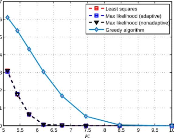
Figure 2: Top: Average error rate of the four estimating procedures in the experiment with heteroscedastic noise as a function of the minimal distanceκbetween distinct fea-tures. Bottom: zoom on the same plots. One can observe that the LSNS and LSL are almost indistinguishable and, as predicted by the theory, perform better than the LSS and the greedy algorithm.

1

n

Pn

i=11(ˆπ(i)6=π∗(i)). The result, averaged over 500 independent trials, is plotted in Fig. 2.

One can observe that among the noise-level-adaptive estimators, LSL outperforms the two others and is as accurate as (and even slightly better than) the LSNS (pseudo)-estimator.

7

Conclusion

Motivated by the problem of feature matching, we pro-posed a rigorous framework for studying the problem of permutation estimation from a minimax point of view. The key notion in our framework is the mini-max rate of identification, which plays the same role as the minimax rate of separation in the statistical hy-potheses testing theory [6]. We established theoretical guarantees for several natural estimators and proved the optimality of some of them. The results appeared to be quite different in the homoscedastic and in the heteroscedastic case. However, we have shown that

the least sum of logarithms estimator outperforms the other procedures either theoretically or empirically.

8

Proofs of Theorems

In this section we collect the proofs of the theorems stated in Section 3.2. We start with the proof of The-orem 3, since it concerns the more general setting and the proof of Theorem 1 follows from that of Theorem 3 by simple arguments. We then prove Theorem 2 and postpone the proofs of some technical lemmas to the appendix.

8.1 Proof of Theorem 3

To ease notation and without loss of generality, we assume that π∗ _{is the identity permutation denoted}

byid. Furthermore, since there is no risk of confusion, we write Pinstead ofPθ,σ,π∗. We wish to bound the probability of the eventΩ ={πˆ6=π∗}.

Let us first denote byπˆ the maximum likelihood esti-matorπLSL _{defined by (6). We have}

Ω = [ π6=id Ωπ, where Ωπ = nXn i=1 log kXi−X # i k 2 kXπ(i)−X # i k2 >0o =n X i:π(i)6=i log kXi−X # i k2 kXπ(i)−X # i k2 >0o.

On the one hand, for every permutation π, using the concavity of the logarithm we get

X π(i)6=i log 2σi2 σ2 i+σ2π(i) = n X i=1 log(2σ_i2)−log(σ_i2+σ_π2_(i)) = n X i=1 log(2σ2 i) + log(2σπ2(i)) 2 −log(σ 2 i +σ 2 π(i)) ≤0. Therefore, Ωπ⊂ n X i:π(i)6=i log kXi−Xi#k2/(2σ2i) kXπ(i)−X # i k2/(σi2+σ2π(i)) >0o ⊂ n [ i=1 [ i6=j nkX_i−X# i k2 2σ2 i > kXj−X # i k2 σ2 j +σ 2 i o .

This readily yieldsΩ⊂Ω, where¯ ¯ Ω = n [ i=1 [ i6=j nkX_i−X# i k2 2σ2 i ≥ kXj−X # i k2 σ2 j+σ 2 i o . (10)

Furthermore, the same inclusion is obviously true for the LSNS estimator as well. Therefore, the rest of the proof is common for the estimators LSNS and LSL. Let us denote ζ1= max i6=j (θi−θj)>(σiξi−σjξj#) kθi−θjk √ σ2 i+σj2 , ζ2=d−1/2max i,j σ_√iξi−σjξj# σ2 i+σ2j 2 −d .

Sinceπ∗=id, for everyi∈ {1, . . . , n}, it holds that kXi−Xi#k 2_=σ2 ikξi−ξi#k 2_≤2σ2 i(d+ √ dζ2). Similarly, for everyj6=i,

kXj−Xi#k 2_=kθ j−θik2+kσjξj−σiξi#k 2 + 2(θj−θi)>(σjξj−σiξi#). Therefore, kXj−X # i k 2 ≥ kθj−θik2+ (σi2+σ 2 j)(d− √ dζ2) −2kθj−θik q σ2_i +σ_j2ζ1.

This implies that on the event Ω1 = {˜κ(θ) ≥ ζ1} it holds that kXj−X # i k 2 σ2 i +σ2j ≥κ˜(θ)2−2˜κ(θ)ζ1+d− √ dζ2.

Combining these bounds, we get that Ω∩Ω1⊂

n d+ √ dζ2 > ˜κ(θ)2−2˜κ(θ)ζ1+d− √ dζ2 o , which implies that P(Ω)≤P(Ω{₁) +P Ω∩Ω1 ≤P ζ1≥˜κ(θ) +P(2√dζ2+ 2˜κ(θ)ζ1>κ˜(θ)2) ≤2P ζ1≥ ˜ κ(θ) 4 +P ζ2> ˜ κ(θ)2 4√d . (11)

Finally, one easily checks that for suitably chosen ran-dom variablesζi,j drawn from the standard Gaussian

distribution, it holds that ζ1 = maxi6=j|ζi,j|.

There-fore, using the well-known tail bound for the standard Gaussian distribution in conjunction with the union bound, we get P ζ1≥1₄κ˜(θ)≤ X i6=j P |ζi,j| ≥ 1₄κ˜(θ) ≤2n2e−321κ˜(θ) 2 . (12)

Similarly, using the tail bound of Lemma 4 stated in the supplementary material and borrowed from Lau-rent and Massart [8], we get

P ζ2>κ˜(θ) 2 4√d ≤2n2e−(˜κ(θ)d/16)2(˜κ 2_(θ)∧8d) . (13)

Combining inequalities (11)-(13), we obtain that as soon as ˜ κ(θ)≥4p2 log(8n2_{/α)∨ dlog(4n}2_/α)1/4 , we have P(ˆπ6=π∗) =P(Ω)≤α. 8.2 Proof of Theorem 1 It is evident that on the event

A= n \ i=1 \ j6=i n kXπ∗_(i)−X_i#k<kX_π∗_(i)−X_j#k o

all the four estimators coincide with the true permu-tationπ∗. Therefore, we have

{πˆ6=π∗} ⊆ n [ i=1 [ j6=i n kXπ∗_(i)−X_i#k>kX_π∗_(i)−X_j#k o .

The latter event coincides with Ω¯ at the right-hand side of (10), the probability of which has been already evaluated in the previous proof. This completes the proof.

8.3 Proof of Theorem 2

For two probability measures P and Q such that P

is absolutely continuous with respect toQ, we denote by K(P,Q)the Kullback-Leibler divergence between

PandQdefined by

K(P,Q) =

Z

logdP

dQ dP.

In our proof, we decided to separate the cases when maxn(logn)1/2, c(dlogn)1/4o= (logn)1/2 and when

maxn(logn)1/2, c(dlogn)1/4o=c(dlogn)1/4.

Besides, we will repeatedly use the fact that forn≥4, log(n/2)≥1

2lognand, to ease notation, we will omit the subscriptσ inPθ,σ,π.

First part: κ≤(σ/4)√logn

Notice that in this first case κ ≤ (σ/√8)plog(n/2), which is the bound we will use from now on.

We choose θ0 ∈ Rn×d such that θ0,i = (i ×

κ,0, . . . ,0)> ∈ Rd for every i ∈ {1, . . . , n}. We

re-duce our problem from considering Θκ to considering

onlyθ0∈Θκ: inf ˆ π _θsup_∈Θ κ max π∗_∈S n Pθ,π∗ πˆ6=π∗ ≥inf ˆ π πmax∗_∈S n Pθ0,π∗ ˆπ6=π ∗ .

A lower bound for this quantity can be obtained from the following lemma:

Permutation estimation and minimax rates of identifiability

Lemma 1(Tsybakov [12]). LetM be an integer larger than 2. Assume that there exist distinct permutations

π0, . . . , πM ∈Sn and mutually absolutely continuous

probability measuresQ0, . . . ,QM such that

1 M M X j=1 K(Qj,Q0)≤ 1 8logM, then inf ˜ π j=0max,...,MQj(˜π6=πj)≥ √ M √ M + 1 3 4− 1 2√logM ,

where the infimum is taken over all permutation esti-mators.

We will apply this lemma with M = n−1 and, for

i= 1, . . . , n,πi being the permutation which leaves all

j ∈ {1, . . . , n} \ {i, i+ 1} invariant and switchesiand

i+ 1. Then, we have K Qi,Q0= 1 2σ2 n X k=1 kθ0,πi(k)−θ0,kk 2_≤ κ2 σ2. Thus, ifn≥3andκ≤(σ/√8)plog(n/2), then

1 M M X i=1 K Qi,Q0 =1 8 log(n/2)≤ 1 8logM and Lemma 1 yields the desired result.

Second part: κ≤(cσ/4)(dlogn)1/4

In this second part, we suppose that c ≤ 1, so that

κ≤(σ/4) dlogn1/4

, which is the bound we need to prove the result. Furthermore, the hypothesis made on the maximum implies that

d≥ 1

c4logn≥logn.

Now, let µ be a (prior) probability measure on

Rn×d. Define the (posterior) probability Pµ,π =

R RndPθ,πµ(dθ). It holds that sup θ∈Θκ max π∗_∈S n Pθ,π∗ πˆ6=π∗ ≥ max π∗_∈{id}∪Π Z Θκ Pθ,π∗ πˆ 6=π µ(dθ) µ(Θκ) ≥ max π∗_∈{id}∪ΠPµ,π ∗ πˆ6=π_j−µ(_Rnd\Θ_κ). We will use Lemma 1 again with

     M =n,

π0=id andπ1, . . . , πM M distinct transpositions,

∀i∈ {0, . . . , M},Qi=Pµ,πi.

To this end, we state the following lemma, that al-lows us to bound the Kullback-Leibler divergence from above.

Lemma 2. Let be a positive real number with ≤

σ/2and letµbe the uniform distribution on{±}n×d_.

Then, for any transposition π, we have

K(Pµ,π,Pµ,id)≤ 8d4 σ4 . Furthermore, if =κ/√d, then µ(Rnd\Θκ)≤ n(n−1) 2 e −d/8_.

Using the priorµ and the value of≤σ/2defined in the previous lemma, we get

1 M M X i=1 K(Qi,Q0)≤ 8d4 σ4 = 8κ4 dσ4 ≤ 1 8logn. This implies that the minimum risk is larger than

√ 3 √ 3 + 1 3 4− 1 2√log 3 −n 2 2 e −d/8_. Finally, remembering thatd≥ 1

c4logn, we have

(n2/2)e−d/8≤ 1 2n

2−1/8c4 .

Takingc small enough, we get the desired result. 8.4 Proof of Theorem 4

It is clear that {πgr _6=π∗_{} ⊃ {kX}

1−X1#k2 >kX1−

X₂#k2_{} := Ω}

2. In the following, we lower bound the probability of the eventΩ2. Let us choose anyθ from

Rn×d satisfyingkθ1−θ2k= 2˜κ.

One easily checks that for suitably chosen random vari-ables η1∼χ2d,η2∼χ2d andζ3∼ N(0,1) it holds that kX1−X1#k

2_{− kX}

1−X2#k 2_{= 6η}

1−4˜κ2−8˜κζ3−4η2. According to Lemma 4 stated in the supplementary material, for every x > 0, each one of the following three inequalities holds true with probability at least 1−e−x2: η1≥d−2 √ dx, η2≤d+ 2 √ dx+ 2x2, ζ3≤ √ 2x.

This implies that with probability at least 1−3e−x2, we have kX1−X1#k 2_{− kX} 1−X2#k 2 ≥2d−20 √ dx−4(˜κ+√2x)2.

If x = √log 6, then the conditions imposed in The-orem 4 on ˜κ and d ensure that the right-hand side of the last inequality is positive. Therefore, P( ¯Ω) ≥ 1−3e−x2= 1/2.

References

[1] H. Bay, A. Ess, T. Tuytelaars and L. Van Gool. SURF: Speeded Up Robust Features.

Com-puter Vision and Image Understanding, 110: 346–359, 2008.

[2] E. Budish, Y.K. Che, F. Kojima and P. Mil-grom. Designing Random Allocation Mechanisms:

Theory and Applications. American Economic

Re-view, to appear, 2012.

[3] O. Collier. Minimax hypothesis testing for curve registration. Electron. J. Statist., 6:1129–1154, 2012. [4] O. Collier and A. Dalalyan.Wilks’ phenomenon and penalized likelihood-ratio test for nonparamet-ric curve registration. Journal of Machine Learning Research - Proceedings Track (AISTATS 2012), 22: 264-272, 2012.

[5] R. Hartley and A. Zisserman. Multiple view

ge-ometry in computer vision. Second edition. Cam-bridge University Press, CamCam-bridge, 2003.

[6] Yu. I. Ingster and I. A. Suslina. Nonparametric

goodness-of-fit testing under Gaussian models. Lec-ture Notes in Statistics. Springer-Verlag, New York, 2003.

[7] Jebara T. Images as Bags of Pixels. Presented at IEEE International Conference on Computer Vision (ICCV’03), 2003.

[8] B. Laurent and P. Massart.Adaptive estimation

of a quadratic functional by model selection. Ann.

Statist., 28:1302–1338, 2000.

[9] D.G. Lowe. Distinctive image features from scale-invariant keypoints.International journal of computer vision, 60 (2):91–110, 2004.

[10] J. F. Sturm. Using SeDuMi 1.02, a MATLAB

tool-box for optimization over symmetric cones. Optim.

Methods Softw., 11/12(1-4):625-653, 1999.

[11] R. Szeliski. Computer Vision: Algorithms and Ap-plications. Springer, New York, 2010.

[12] A.B. Tsybakov.Introduction to Nonparametric Es-timation. Springer Verlag, 2008.

Appendix

Lemma 3. For every x∈R, it holds that x2 2 − x4 12 ≤log cosh(x)≤ x2 2 .

Lemma 4 (Laurent and Massart [8]). Let Y ∼

χ2_{(D), whereD∈}

N∗. Then, for everyx >0,    P Y −D≤ −2√Dx≤e−x, P Y −D≥2√Dx+ 2x ≤e−x_.

As a consequence, for every y >0,

P D−1/2|Y −D| ≥y

≤2 expn−1 8y(y∧

√

D)o.

Proof of Lemma 2. Let π be the transposition (i, j). Let θ = (θ1, . . . , θn) be randomly drawn from

µ. We define θ0 by θ0

i = θ0j = 0 and θ0k = θk

if k 6∈ {i, j}. Let us denote by µ˜ the probability distribution of this random matrix on _Rn×d and set

Pµ,π˜ =

R

ΘPθ,π µ˜(dθ).

We first compute the likelihood ratio of Pµ,π

and Pµ,id. We get, for every (X, Y) =

(X1, . . . , Xn, Y1, . . . , Yn)inRnd, dPµ,π dPµ,id (X, Y) =dPµ,π dPµ˜ (X, Y)×dPµ,id dPµ˜ (X, Y) −1 =Eµ " dPθi dP0 (Xi) dPθj dP0 (Xj) dPθj dP0 (Yi) dPθi dP0 (Yj) # ×E−_µ1 " dPθi dP0 (Xi) dPθj dP0 (Xj) dPθi dP0 (Yi) dPθj dP0 (Yj) # .

Now, reminding that for example

dPθi dP0 (Xi) =e− 2d 2σ2+σ12(Xi,θi)_, we get that dPµ,π dPµ,id (X, Y) = d Y k=1 cosh _σ2(X (k) i +Y (k) j ) cosh _σ2(X (k) i +Y (k) i ) × d Y k=1 cosh _σ2(X (k) j +Y (k) i ) cosh _σ2(X (k) j +Y (k) j ) .

Then, we compute the Kullback-Leibler divergence,

K(Pµ,π,Pµ,id) = Z logdPµ,π dPµ,id dPµ,π = 2 d X k=1 Eµ hZ log cosh σ2(2θi,k+σ √ 2X)dQi −2 d X k=1 Eµ hZ log cosh σ2(θi,k+θj,k+σ √ 2X)dQi,

where Q is a standard Gaussian distribution. Using Lemma 3, we get that the general term in the first sum is smaller than 2

σ2+2

4

σ4, while the second general term

is larger than _σ22 −2 6 σ6 − 2 3 8 σ8, whence K(Pµ,π,Pµ,id)≤4d 4 σ4 + 4d 6 σ6+ 4d 3 8 σ8 ≤ 8d4 σ4 . Finally, to upper boundµ(Rnd\Θκ), we notice that

µ(Rnd\Θκ)≤ n(n−₂ 1)µ kθ1−θ2k2< κ2 ≤ n(n−₂ 1)µ d P j=1 (ζ₁(j)−ζ₂(j))2< κ22 =d .