Classification of Hyperspectral Images
Gabriele Cavallaro, Mauro Dalla Mura, Jon Atli Benediktsson, Lorenzo
Bruzzone
To cite this version:
Gabriele Cavallaro, Mauro Dalla Mura, Jon Atli Benediktsson, Lorenzo Bruzzone. Extended
Self-Dual Attribute Profiles for the Classification of Hyperspectral Images. IEEE Geoscience
and Remote Sensing Letters, IEEE - Institute of Electrical and Electronics Engineers, 2015,
<
10.1109/LGRS.2015.2419629
>
.
<
hal-01259781
>
HAL Id: hal-01259781
https://hal.archives-ouvertes.fr/hal-01259781
Submitted on 20 Jan 2016
HAL
is a multi-disciplinary open access
archive for the deposit and dissemination of
sci-entific research documents, whether they are
pub-lished or not.
The documents may come from
teaching and research institutions in France or
abroad, or from public or private research centers.
L’archive ouverte pluridisciplinaire
HAL
, est
destin´
ee au d´
epˆ
ot et `
a la diffusion de documents
scientifiques de niveau recherche, publi´
es ou non,
´
emanant des ´
etablissements d’enseignement et de
recherche fran¸
cais ou ´
etrangers, des laboratoires
publics ou priv´
es.
Extended Self-Dual Attribute Profiles for the
Classification of Hyperspectral Images
Gabriele Cavallaro,
Student Member, IEEE,
Mauro Dalla Mura,
Member, IEEE,
J´on Atli Benediktsson,
Fellow, IEEE,
and Lorenzo Bruzzone,
Fellow, IEEE,
Abstract—In this letter, we explore the use of self-dual attribute
profiles (SDAPs) for the classification of hyperspectral images. The hyperspectral data are reduced into a set of components by non-parametric weighted feature extraction (NWFE), and a morphological processing is then performed by the SDAPs separately on each of the extracted components. Since the spatial information extracted by SDAPs results in a high number of features, the NWFE is applied a second time in order to extract a fixed number of features, which are finally classified. The experiments are carried out on two hyperspectral images, and the support vector machines (SVMs) and Random Forest (RF) are used as classifiers. The effectiveness of SDAPs is assessed by comparing its results against those obtained by an approach based on extended attribute profiles (EAPs).
Index Terms—Attribute filters, attribute profiles, self-dual
attribute profiles, extended attribute profiles, non-parametric weighted feature extraction, mathematical morphology, remote sensing.
I. INTRODUCTION
T
HE DEVELOPMENT in hyperspectral sensors is leading to an increased availability of data having both high spectral and spatial resolution. The high spectral resolution (i.e., hundreds of channels acquired in very narrow spectral bands) allows a very accurate identification of surface mate-rials. The high spatial resolution enables precise analysis of small heterogeneous spatial structures present in the surveyed scene. The modeling of the characteristics of spatial objects can be achieved by processing an image with a set of math-ematical morphology operators. In this context, region-based filtering tools [1] (called connected operators) have recently received significant attention due to their effectiveness in both extracting spatial information and preserving the geometrical characteristics of the objects in images (i.e., borders of regions are not distorted since only an image is processed by merging its flat zones). Attribute filters [2] are a set of connected operators that are able to simplify a grayscale image accordingG. Cavallaro is with the Faculty of Electrical and Computer Engi-neering, University of Iceland, Reykjavik 101, Iceland (e-mail: [email protected]).
M. Dalla Mura is with the GIPSA-lab, Grenoble Institute of Technology, Grenoble, France (e-mail: [email protected]).
J. A. Benediktsson is with the Engineering Research Institute, University of Iceland, Reykjavik 107, Iceland (e-mail: [email protected]).
L. Bruzzone is with the Department of Information and Communi-cation Technologies, University of Trento, 38050 Trento, Italy (e-mail: [email protected]).
This research was supported in part by EU FP7 Theme Space project North State and the program J. Verne 2014 under Project 31936TD. The authors are grateful to professor Bor-Chen Kuo for providing the NWFE code.
to an arbitrary measure (i.e., attribute), such as scale, shape and contrast. In Dalla Mura et al. [3], the authors proposed to use attribute filters in a multilevel approach, called attribute profiles (APs), for dealing with the heterogeneity of objects present in remote sensing high resolution images (both in scale and shape). Dalla Muraet al.[4] showed interesting properties of APs when extended to hyperspectral images (EAPs) and used as spatial features for classification. Dalla Mura et al.
[4] [5] applied APs to the first few principal components (i.e., PCA) and to the independent components (i.e., ICA), extracted from a hyperspectral image, respectively. Dalla Muraet al.[6] proposed self-dual attribute profiles with area attribute as a variant of APs for the classification of very high geometrical resolution images. The use of SDAPs proved to be more effective than APs for modeling the spatial information (i.e., bright and dark regions are simultaneously processed) even with a reduced number of features. Subsequently, Cavallaro
et al. [7] compared APs with SDAPs obtained by different attributes and filtering strategies and showed that SDAPs could achieve higher classification accuracy. In this letter, we propose Extended Self-Dual Attribute Profiles (ESDAPs), a generalization of SDAPs for the extraction of spatial features for the classification of hyperspectral images. A classic ap-proach extracting spectral-spatial classification based on a two-steps supervised feature extraction technique [8] is adopted with the non-parametric weighted feature extraction NWFE method [9]. We aim to compare the capability of extracting the spatial information of EAPs and ESDAPs components when considering different attributes. This is done by analyzing at the classification accuracies provided by the support vector machines (SVM) and Random Forest (RF) classifiers. The remainder of this letter is organized as follows. Section II reviews the features reduction methods by focusing on the supervised NWFE. The concepts of morphological attribute filters and extended self-dual attribute profiles (ESDAPs) are introduced in section III. The experimental analysis (which includes the description of the data sets), the setup and the results are described in section IV. Section V concludes this letter with some remarks and possible future research directions.
II. FEATUREEXTRACTION
Feature extraction in hyperspectral images is an impor-tant processing step that can improve the effectiveness of a classifier [10]. Several approaches have been developed to address this task. They are typically based on statistical
methods, which might face significant challenges especially when dealing with data of high dimensionality [11]. Data mining techniques are included in the classification of remote sensing images for two main reasons: to counteract the Hughes phenomenon [12] (i.e., the combination of high dimensional data and a small number of training samples) and to reduce the required computational load. Data mining techniques present in the literature include supervised and unsupervised, paramet-ric and nonparametparamet-ric, linear and nonlinear methods, which all seek to identify the relevant informative subspace. Indeed, the original feature space may not be the most effective domain for representing hyperspectral data. This work adopts the Non-parametric Weighted Feature Extraction (NWFE) technique which is an efficient algorithm for high dimensional multi-class pattern recognition problems [10]. NWFE is a supervised method (i.e., it computes the transformation according to the properties of the training set), and assigns different weights to each sample in order to compute the weighted means. Since NWFE is based on a nonparametric extension of scatter matrices (i.e., between-class and within-class), the algorithm is able to extract a desired number of features (higher than the number of classes) and can work well even for data that are not in Gaussian distribution [10].
III. DEFINITION OFEXTENDEDSDAPS
We define Extended Self-Dual Attribute Profile as an ex-tension of SDAPs for the analysis of hyperspectral images. ESDAPs are based on morphological attribute filters applied on the Inclusion tree, which is a hierarchical representation of the image [13].
Attribute filters (AFs) are a set of connected operators defined in the mathematical morphology framework [14]. They proved to be effective tools for the analysis of the spatial information in images. Connected operators process an image by removing flat zones (i.e., a set of connected iso-intensity pixels) according to a given criterion T based on a single or multiple attributes (e.g., geometrical, textural and spectral). Since only flat zones can be processed, the result of the filtering preserves geometrical features such as the borders. Attribute filters can be efficiently implemented on an equivalent representation of an image, such as the component tree (i.e., min-tree or max-tree [15]) or the inclusion tree (also known as tree of shapes) [13]. The representation of the image as max-tree (min-tree) can be used to perform an attribute thinning γT (thickening φT), which is an
anti-extensive (anti-extensive) idempotent transformation [3]. Self-dual connected operatorsρT [6] can be obtained by considering the inclusion tree representation since it stores both the min- and max-trees.
The application of attribute filters on a given tree structure is composed by the following three steps:
1) Compute the tree representation of the image (i.e., identification of connected components and modeling the hierarchical structure between the components). 2) Pruning the tree by removing the nodes whose associated
regions do not fulfill a given binary predicate T. The predicate usually compares an attribute αcomputed on
the pixels corresponding to a node X in the tree and gives the threshold value taken as reference λ: e.g.,
T =α(X)≥λ.
3) Converting the pruned tree back to the image.
A. Tree representations
Mathematical morphology provides a model for represent-ing images by usrepresent-ing structure level sets [16]. A discrete two-dimensional grayscale image can be fully represented by sets of connected components (i.e., lower and upper level sets [17]) obtained by a thresholding computed over all the values within the image. An inclusion relationship between the extracted connected components allows to associate each of them to a node of a tree and to represent the image as a hierarchical structure. The min-tree and max-tree represent the components in the lower and upper level sets, respectively. The min-tree models the inclusion of regions according to decreasing ordering relation among the graylevel (i.e., ≤), therefore the tree contains only the shapes that are darker than their neighborhood (i.e., the graylevel of each region is lower than their neighborhood graylevel). The max-tree is dual and contains only the regions that are brighter than the graylevel of their neighboring pixels. These trees are complementary representations of the image, since usually not all the components present in the min-tree are also present in the max-tree and vice versa. A more general representation of the image is given by the inclusion tree, a quasi self-dual representation [13], which includes both min-tree and max-tree in a single structure. An operation called saturation is applied to the connected components. It gives flat regions that are obtained by progressively merging nested regions. The inclusion tree can be built by an efficient algorithm called Fast Level Sets Transform (FLST) [13]. The inclusion tree is a complete representation of the input image meaning that the image can be fully retrieved from the tree.
B. APs and SDAPs
Attribute profiles are introduced in remote sensing in [18] as a sequential application of attribute filters based on a min-tree (i.e., attribute thickening operation φT) and max-tree
(i.e., attribute thinning operationγT). The AP is obtained by
filtering an imageuwith attribute operators using a predicate with increasing threshold values{λk}1L:
AP(u) ={φTλL(u), φTλL−1(u), ..., u, ..., γTλL−1(u), γTλL(u)} (1)
withφandγbeing the thickening and thinning operators based on the predicate T, respectively, and Tλ a set of L ordered
predicates.
APs provide a multilevel characterization of the spatial fea-tures which can be useful for the classification of very high resolution remote sensing images [18].
The Self-Dual Attribute Profiles [6], are proposed as a version of the APs based on self-dual connected operators
ρT computed on the inclusion tree of the image instead of considering a min-tree or max-tree. The use of the inclusion
tree as a structure representing the image allows simultane-ously to access the information present on both min-tree and max-tree. Moreover, the self-dual connected operators that are computed on the inclusion tree produce a greater simplification of the image with respect to non dual filters, since they operate simultaneously on bright and dark components of the image. SDAPs is obtained by filtering an image u with attribute operators using a predicate with increasing threshold values:
SDAP(u) ={u, ρTλ1(u), ..., ρTλL−1(u), ρTλL(u)} (2)
withρbeing the self-dual operator based on the predicateT, andTλ a set ofL ordered predicates.
Dalla Muraet al.in [4] proposed extended attribute profiles (EAPs) as the application of APs to hyperspectral data. An EAP is obtained by concatenating the APs (i.e., based on a single attribute) built on several feature components (FCs) extracted by a reduction technique (i.e., PCA) computed on the hyperspectral image. Thus, the EAP can be formally defined as:
EAP ={AP(F C1), AP(F C2), ..., AP(F CN)} (3)
An example of EAPs derived from the first two feature components with the moment of inertia attribute is reported in Fig. 1.
Analogously to the definition of EAP, we propose Extended Self-Dual Attribute Profiles which are generated by concate-nating the SDAPs computed on different components. Each SDAP is built on one of theN features components extracted by a feature reduction transformation from a hyperspectral image:
ESDAP ={SDAP(F C1), SDAP(F C2), ..., SDAP(F CN)}
(4) An example of ESDAP, derived from the first two feature components with themoment of inertiaattribute is reported in Fig. 2. In contrast to APs, the SDAPs are composed ofN+ 1
images while APs, built with the same sequence of λs are
made up of 2N+ 1 images. 𝑆𝑆𝑆𝑆𝑆𝑆𝑆𝑆(𝑆𝑆𝐶𝐶1) 𝑆𝑆𝑆𝑆𝑆𝑆𝑆𝑆(𝑆𝑆𝐶𝐶2) 𝑆𝑆𝑆𝑆𝑆𝑆𝑆𝑆(𝑆𝑆𝐶𝐶3) 𝑆𝑆𝑆𝑆𝑆𝑆𝑆𝑆(𝑆𝑆𝐶𝐶4) 𝐹𝐹𝐶𝐶1 𝜙𝜙𝑇𝑇𝜆𝜆4(𝐹𝐹𝐶𝐶1) 𝜙𝜙𝑇𝑇𝜆𝜆3(𝐹𝐹𝐶𝐶1) 𝜙𝜙𝑇𝑇𝜆𝜆2(𝐹𝐹𝐶𝐶1) 𝜙𝜙𝑇𝑇𝜆𝜆1(𝐹𝐹𝐶𝐶1) 𝛾𝛾𝑇𝑇𝜆𝜆1(𝐹𝐹𝐶𝐶1) 𝛾𝛾𝑇𝑇𝜆𝜆2(𝐹𝐹𝐶𝐶1) 𝛾𝛾𝑇𝑇𝜆𝜆3(𝐹𝐹𝐶𝐶1) 𝛾𝛾𝑇𝑇𝜆𝜆4(𝐹𝐹𝐶𝐶1) 𝐹𝐹𝐶𝐶2 𝜙𝜙𝑇𝑇𝜆𝜆4(𝐹𝐹𝐶𝐶2) 𝜙𝜙𝑇𝑇𝜆𝜆3(𝐹𝐹𝐶𝐶2) 𝜙𝜙𝑇𝑇𝜆𝜆2(𝐹𝐹𝐶𝐶2) 𝜙𝜙𝑇𝑇𝜆𝜆1(𝐹𝐹𝐶𝐶2) 𝛾𝛾𝑇𝑇𝜆𝜆1(𝐹𝐹𝐶𝐶2) 𝛾𝛾𝑇𝑇𝜆𝜆2(𝐹𝐹𝐶𝐶2) 𝛾𝛾𝑇𝑇𝜆𝜆3(𝐹𝐹𝐶𝐶2) 𝛾𝛾𝑇𝑇𝜆𝜆4(𝐹𝐹𝐶𝐶2)
Fig. 1. Example of EAP computed on the first two FCs extracted by NWFE from the Indian Pines data set. The EAP is generated by the concatenation of four APs derived fromF C1andF C2. Each AP is composed of three levels:
A thickening imageφT, the original FC, and theγT image. All the filtering
φT andγT are computed withmoment of inertiaand the threshold values shown in Table III
IV. EXPERIMENTAL ANALYSIS
A. Data sets
The experimental analysis has been carried out on two hyperspectral images acquired by the AVIRIS and ROSIS
𝑆𝑆𝑆𝑆𝑆𝑆𝑆𝑆(𝑆𝑆𝐶𝐶1) 𝑆𝑆𝑆𝑆𝑆𝑆𝑆𝑆(𝑆𝑆𝐶𝐶2) 𝑆𝑆𝑆𝑆𝑆𝑆𝑆𝑆(𝑆𝑆𝐶𝐶3) 𝑆𝑆𝑆𝑆𝑆𝑆𝑆𝑆(𝑆𝑆𝐶𝐶4)
𝐹𝐹𝐶𝐶1 𝜌𝜌𝑇𝑇𝜆𝜆1(𝐹𝐹𝐶𝐶1) 𝜌𝜌𝑇𝑇𝜆𝜆2(𝐹𝐹𝐶𝐶1) 𝜌𝜌𝑇𝑇𝜆𝜆3(𝐹𝐹𝐶𝐶1) 𝜌𝜌𝑇𝑇𝜆𝜆4(𝐹𝐹𝐶𝐶1)
𝐹𝐹𝐶𝐶2 𝜌𝜌𝑇𝑇𝜆𝜆1(𝐹𝐹𝐶𝐶2) 𝜌𝜌𝑇𝑇𝜆𝜆2(𝐹𝐹𝐶𝐶2) 𝜌𝜌𝑇𝑇𝜆𝜆3(𝐹𝐹𝐶𝐶2) 𝜌𝜌𝑇𝑇𝜆𝜆4(𝐹𝐹𝐶𝐶2)
Fig. 2. Example of ESDAP computed on the first two FCs extracted by NWFE from Indian Pines data set. The ESDAP is generated by the concatenation of four SDAPs derived fromF C1 andF C2. Each SDAP is composed of two
levels: The original FC, and theρT image. All the filtering are computed
withmoment of inertiaand the threshold values shown in Table III
sensors, respectively. The former captured a scene of the Indian Pines, Indiana, and is made up of 145×145 pixels and 200 spectral bands (with spatial resolution 20 m). The latter represents a portion of the city of Pavia, Italy, and is made up of 640 × 340 pixels with 103 data channels and a spatial resolution of 1.3 m. The Pavia and Indian Pines ground reference data contain 9 and 16 classes (see Fig. 4(a) and Fig. 5(a)), respectively (further information can be found in [5] and [19]). The experiments for Indian Pines are run ten times with a set of different training sets randomly selected (10% of the labeled samples are taken for each class), while for Pavia, the classifier used the training set available with the data [20].
B. Experimental setup
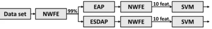
In order to deal with the dimension of the original data and with the elevated number of features extracted by the morphological processing (i.e., EAP and ESDAP), we propose the flowchart shown in Fig. 3. The hyperspectral data sets are reduced by NWFE into a subspace of feature components (FCs). The AP and SDAP are applied to the first FCs, which contain more than 99% of the total variance of the data. This leads to the definition of EAP and ESDAP, respectively. Finally, since the EAP and the ESDAP built on the different extracted components result in a high number of features, the NWFE is performed for the second time, with only the first 10 features selected to be classified (to ensure fair comparison of the capability in modeling the spatial information between EAP and ESDAP).
Data set NWFE EAP ESDAP
NWFE 10 feat. SVM
99%
NWFE 10 feat. SVM
Fig. 3. Flowchart of the spectral-spatial classification approach based on the two-steps supervised NWFE.
For all the experiments, the Leave-One-Out Covariance (LOOC) estimator is applied to regularize the within-class scatter matrix for the performances of the NWFE (i.e., neces-sary in small training sample size situation). The mixing pa-rameterβ [21] is fixed at 0.5. For both data sets, the EAP and ESDAP were computed on the feature components extracted by NWFE considering attribute and threshold values reported
TABLE I
PAVIA UNIVERSITY DATA SET. CLASSIFICATION ACCURACIES OBTAINED BY CLASSIFYING WITHSVMANDRFTHE HYPERSPECTRAL IMAGE(RAW),THE FIRST FEATURE COMPONENTS WHICH CONTAIN MORE THAN99%OF THE TOTAL VARIANCE OF THE DATA(FE),EACH SINGLEEAP,EACH SINGLE
ESDAP,AND THE STACKED VECTOR WHICH CONCATENATES THE DIFFERENT ATTRIBUTES.
Classifier Features Raw (103) FE (11) EAPaFE (10) EAPdFE (10) EAPiFE (10) EAPsFE (10) ESDAPaFE (10) ESDAPdFE (10) ESDAPiFE (10) ESDAPsFE (10) SV EAP (40) SV ESDAP (40) K (%) 75.11 74.41 92,51 88,67 83,83 86,48 95,22 90,21 86,48 94,51 87,14 91,37 SVM OA (%) 80.05 79.51 94,31 91,28 87,24 89,52 96,41 92,44 89,51 95,82 89,95 93,39 AA (%) 88.03 87.69 94,44 92,91 94,06 90,91 96,27 94,71 93,33 94,81 95,16 95,53 K (%) 65,33 71,09 91,22 88,34 87,83 87,03 94,34 94,15 86,14 89,98 93,79 97,22 RF OA (%) 71,82 76,58 93,34 90,98 90,52 89,95 95,75 95,57 89,22 92,23 95,26 97,89 AA (%) 82,31 86,65 92,17 93,37 94,12 91,28 93,82 94,51 91,24 95,77 95,32 97,74 TABLE II
INDIANPINES DATA SET. CLASSIFICATION ACCURACIES OBTAINED BY CLASSIFYING WITHSVMANDRFTHE HYPERSPECTRAL IMAGE(RAW),THE FIRST FEATURE COMPONENTS WHICH CONTAIN MORE THAN99%OF THE TOTAL VARIANCE OF THE DATA(FE),EACH SINGLEEAP,EACH SINGLE
ESDAP,AND THE STACKED VECTOR WHICH CONCATENATES THE DIFFERENT ATTRIBUTES(MEAN AND STANDARD DEVIATION IN BRACKET).
Classifier Features Raw (200) FE (123) EAPaFE (10) EAPdFE (10) EAPiFE (10) EAPsFE (10) ESDAPaFE (10) ESDAPdFE (10) ESDAPiFE (10) ESDAPsFE (10) SV EAP (40) SV ESDAP (40) K (%) 78,42 (0,76) 72,07 (1,23) 81,42 (1,61) 81,05 (1,56) 81,59 (0,99) 83,89 (1,16) 93,21 (0,88) 93,55 (1,02) 83,57 (1,13) 91,84 (0,82) 90,88 (1,21) 96,05 (0,15) SVM OA (%) 81,11 (0,66) 75,71 (1,06) 83,78 (1,39) 83,47 (1,65) 83,97 (0,86) 85,91 (1,03) 94,05 (0,77) 94,36 (0,89) 85,68 (0,97) 92,85 (0,72) 92,05 (1,04) 96,54 (0,13) AA (%) 77,04 (1,88) 64,37 (1,75) 73,78 (3,32) 72,48 (3,17) 77,09 (4,17) 82,77 (2,61) 89,16 (2,82) 88,72 (2,66) 75,67 (4,71) 91,26 (1,15) 76,41 (5,51) 90,74 (3,14) K (%) 71,47 (0,66) 68,61 (1,27) 81,18 (1,03) 79,73 (1,45) 80,27 (1,15) 83,45 (1,11) 92,06 (1,01) 93,12 (0,64) 81,99 (0,72) 90,93 (0,84) 88,41 (0,92) 95,31 (0,51) RF OA (%) 75,29 (0,55) 73,16 (1,05) 83,57 (0,91) 82,34 (1,25) 82,83 (0,99) 85,57 (0,96) 93,04 (0,88) 93,97 (0,55) 84,33 (0,61) 92,06 (0,73) 89,87 (0,81) 95,88 (0,44) AA (%) 61,43 (1,98) 57,21 (1,72) 79,58 (2,33) 78,34 (2,28) 79,27 (2,01) 83,22 (1,84) 93,16 (2,08) 94,09 (1,59) 81,71 (1,21) 90,46 (1,71) 85,13 (1,52) 94,51 (1,82)
in Tab. III (the thresholds were manually selected by a visual analysis of the scenes). The area (i.e. EAPa and ESDAPa)
and thelength of the diagonal(i.e. EAPd and ESDAPd) allow
the extraction of objects based on their size. The moment of inertia(i.e. EAPi and ESDAPi) can describe the geometry of
structures (i.e., elongated objects can be discriminated from compact ones) [22]. Finally,standard deviation(i.e. EAPsand
ESDAPs) can model the homogeneity of the pixels gray levels
belonging to different regions. The stacked vector approach, which was applied in [5], is considered here in order to concatenate the different EAP and ESDAP in a simple vector of features.
TABLE III
ATTRIBUTE AND THRESHOLD VALUES Attribute Pavia Indian
Area 100, 1000, 1500, 2000 50, 100, 500, 2000 Length of the diagonal 10, 25, 50, 100 25, 50, 100, 150
Standard Deviation 5, 7.5 ,10, 12.5 5, 10, 15, 20 Moment of Inertia 0.20, 0.30, 0.40, 0.50 0.18, 0.20, 0.30, 0.40
For each experiment, the performance is reported in terms of overall accuracy (OA), average accuracy (AA) and the Kappa coefficient (K) obtained by the Support Vector Machines (SVMs) and Random Forest (RF) classifiers. For the SVM, the Radial Basis Function (RBF) kernel is adopted, and the regularization C and kernel γ parameters are estimated by exploiting a grid search using a 10-fold cross-validation. The RF classifier is composed by 150 trees.
C. Experimental results
In order to evaluate the performance of SDAPs for the clas-sification of hyperspectral images, we compare the accuracies obtained by ESDAPattr with the results given by EAPattr
(i.e., same attributes and threshold values). The classification
(a) (b) (c)
Fig. 4. Pavia data set. Ground reference (a), classification maps obtained by (b) EAPa (OA 94.31%) and (c) ESDAPa (OA 96.41%) with the SVM
classifier.
(a) (b) (c)
Fig. 5. Indian Pines data set. Ground reference (a), classification maps obtained by (b) EAPs (average OA 85.91%) and (c) ESDAPd(average OA
94.36%) with the SVM classifier..
accuracies are reported in Tables I and II for Pavia and Indian Pines data sets, respectively. For both cases, we report the accuracies achieved with the original data (i.e., 103 and 200 spectral bands) and with the feature components extracted by NWFE in the first step. The spectral channels do not provide enough information to the classifier to achieve very high accuracies. However, the NWFE performs a very efficient
extraction of most of the information components leading to similar results that are generated by the whole spectral infor-mation. In spite of the different data sets, when considering the single EAPattrand ESDAPattr, the information given as input
to the classifier is more complete (i.e., spectral and spatial features), and an improvement in the overall classification accuracies is achieved. For each experiment (i.e., attribute), the EAPattr and ESDAPattr are generated on the extracted
features components (i.e., which contain more than 99% of the total variance of the data), and the NWFE is applied a second time. In order to better investigate the capability of the extended profiles in extracting informative features, the classification step is carried out with a reduced number of FEs provided by the second-step NWFE. In particular, since the variance of the data changes among the different profiles (i.e., EAPattr and ESDAPattr) and attributes, the Tables I
and II report the accuracies obtained by classifying only the first 10 feature components. In the case of a single attribute, for the Indian Pines data set, ESDAPd outperforms the rest of
the attributes (OA of 94,36% and 93,97% for SVM and RF, respectively) while in the Pavia data set the best accuracy is provided by ESDAPa(OA of 96,41% and 95,75% for the SVM
and the RF, respectively). In both cases, the corresponding ESDAPd and ESDAPa perform better than EAPd and EAPa
(see the corresponding classification maps in Fig. 5 and Fig. 4 for the SVM classifier). The stacked vector approach gives the best results in the Indian Pines data set (both classifiers) and in the Pavia University data set (RF classifier) for the ESDAPattr. For the other cases, the information extracted
by the different attributes is redundant, thus penalizing the generalization capability of the classification algorithms (i.e., Hughes phenomenon). In all the experiments, the capability of SDAPattr in modeling the information within heterogeneous
scenes (i.e., feature components) is noticeable. In [6] and [7], it was already shown that spatial information can be better modeled by SDAPattreven with a reduced number of features
with respect to considering the APattr. The experimental
results show that this property holds also for the extended version of the SDAPattr (i.e., ESDAPattr) in the case of
different attributes, data sets and classifiers. V. CONCLUSION
In this paper, we presented the extended self-dual attribute profiles as the extended concept of self-dual attribute profiles for the classification of hyperspectral images. Non-parametric weighted feature extraction (NWFE) was adopted in a two-step fashion: i) for reducing the number of features contained in the original data and ii) for extracting a fixed number of features (i.e., 10) from the different morphological profiles. We proved that in a hyperspectral domain, SDAPs (i.e., multilevel application of attribute filters based on inclusion tree) are a more efficient tool for the analysis of the spatial information than APs. Our future research aims to explore new strategies for the selection of the threshold values by exploring the information present in the inclusion tree structure.
REFERENCES
[1] P. Salembier and J. Serra, “Flat zones filtering, connected operators, and filters by reconstruction,”IEEE Trans on Image Processing, vol. 4, pp. 1153–1160, 1995.
[2] E. J. Breen and R. Jones, “Attribute openings, thinnings, and granulome-tries,”Computer Vision and Image Understanding, vol. 64, no. 3, pp. 377 – 389, 1996.
[3] M. Dalla Mura, J. A. Benediktsson, B. Waske, and L. Bruzzone, “Morphological attribute profiles for the analysis of very high resolution images,”IEEE Transactions on Geoscience and Remote Sensing, vol. 48, no. 10, pp. 3747–3762, Oct 2010.
[4] M. Dalla Mura, J. A. Benediktsson, B. Waske, and L. Bruzzone, “Extended profiles with morphological attribute filters for the analysis of hyperspectral data,”International Journal of Remote Sensing, vol. 31, no. 22, pp. 5975–5991, 2010.
[5] M. Dalla Mura, A. Villa, J. A. Benediktsson, J. Chanussot, and L. Bruzzone, “Classification of hyperspectral images by using extended morphological attribute profiles and independent component analysis,”
Geoscience and Remote Sensing Letters, IEEE, vol. 8, no. 3, pp. 542– 546, May 2011.
[6] M. Dalla Mura, J. A. Benediktsson, and L. Bruzzone, “Self-dual attribute profiles for the analysis of remote sensing images,” in Mathematical Morphology and Its Applications to Image and Signal Processing, P. Soille, M. Pesaresi, and G. Ouzounis, Eds. Springer Berlin Heidelberg, 2011, pp. 320–330.
[7] G. Cavallaro, M. Dalla Mura, J. A. Benediktsson, and L. Bruzzone, “A comparison of self-dual attribute profiles based on different filter rules for classification,”Proceedings of IEEE International Geoscience and Remote Sensing Symposium (IGARSS), pp. 1265–1268, 2014. [8] P. Ghamisi, J. Benediktsson, G. Cavallaro, and A. Plaza, “Automatic
framework for spectral-spatial classification based on supervised fea-ture extraction and morphological attribute profiles,”IEEE Journal of Selected Topics in Applied Earth Observations and Remote Sensing, vol. 7, no. 6, pp. 2147–2160, June 2014.
[9] T. Castaings, B. Waske, J. Atli Benediktsson, and J. Chanussot, “On the influence of feature reduction for the classification of hyperspectral images based on the extended morphological profile,” International Journal of Remote Sensing, vol. 31, no. 22, pp. 5921–5939, 2010. [10] B. C. Kuo and D. Landgrebe, “Nonparametric weighted feature
extrac-tion for classificaextrac-tion,”IEEE Transactions on Geoscience and Remote Sensing, vol. 42, no. 5, pp. 1096–1105, May 2004.
[11] J. Xiuping, K. Bor-Chen, and M. Crawford, “Feature mining for hyper-spectral image classification,”Proceedings of the IEEE, vol. 101, no. 3, pp. 676–697, March 2013.
[12] G. Hughes, “On the mean accuracy of statistical pattern recognizers,”
IEEE Transactions on Information Theory,, vol. 14, no. 1, pp. 55–63, Jan 1968.
[13] P. Monasse and F. Guichard, “Fast computation of a contrast-invariant image representation.”IEEE Trans. Image Processing, vol. 9, pp. 860– 872, 2000.
[14] J. Serra, Image analysis and mathematical morphology. New York: Academic Press, 1982, vol. 1.
[15] P. Salembier, “Connected operators based on region-trees,” pp. 2176– 2179, Oct 2008.
[16] G. Matheron,Random sets and integral geometry [by] G. Matheron. Wiley New York, 1974.
[17] V. Caselles and P. Monasse, Geometric Description of Images as Topographic Maps. Springer Berlin Heidelberg, 2010, vol. 1984. [18] M. Dalla Mura, J. A. Benediktsson, B. Waske, and L. Bruzzone,
“Mor-phological Attribute Profiles for the Analysis of Very High Resolution Images,”IEEE Trans. on Geosci. and Remote Sens., vol. 48, pp. 3747– 3762, 2010.
[19] B. Song, J. Li, M. Dalla Mura, P. Li, A. Plaza, J. Bioucas-Dias, J. A. Benediktsson, and J. Chanussot, “Remotely sensed image classification using sparse representations of morphological attribute profiles,”IEEE Transactions on Geoscience and Remote Sensing, vol. 52, no. 8, pp. 5122–5136, Aug 2014.
[20] P. Gamba. Hyperspectral remote sensing scenes. [Online]. Available: http://www.ehu.es/ccwintco/index.php
[21] B.-C. Kuo and K.-Y. Chang, “Feature extractions for small sample size classification problem,”IEEE Transactions on Geoscience and Remote Sensing, vol. 45, no. 3, pp. 756–764, March 2007.
[22] H. Ming-Kuei, “Visual pattern recognition by moment invariants,”IRE Transactions on Information Theory, vol. 8, no. 2, pp. 179–187, February 1962.