Miao_unc_0153D_15289.pdf

CLASS-SENSITIVE PRINCIPAL COMPONENTS ANALYSIS

Di Miao

A dissertation submitted to the faculty at the University of North Carolina at Chapel Hill in

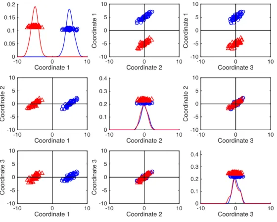
partial fulfillment of the requirements for the degree of Doctor of Philosophy in the

Department of Statistics and Operations Research.

Chapel Hill

2015

Approved by:

J. S. Marron

Jason P. Fine

Andrew B. Nobel

Yufeng Liu

c

2015

Di Miao

ABSTRACT

DI MIAO: CLASS-SENSITIVE PRINCIPAL COMPONENTS ANALYSIS

(Under the direction of J. S. Marron and Jason P. Fine)

Research in a number of fields requires the analysis of complex datasets. Principal

Com-ponents Analysis (PCA) is a popular exploratory method. However it is driven entirely by

variation in the dataset without using any predefined class label information. Linear

clas-sifiers make up a family of popular discrimination methods. However, these will face the

data piling issue often when the dimension of the dataset gets higher. In this dissertation, we

first study the geometric representation of an interesting dataset with strongly auto-regressive

errors under the High Dimensional Low Sample Size (HDLSS) setting and understand why

the Maximal Data Piling (MDP), proposed by Ahn et al. (2007), is the best in terms of

clas-sification compared with several other commonly used linear discrimination methods. Then

we introduce the Class-Sensitive Principal Components Analysis (CSPCA), which is a

com-promise of PCA and MDP, that seeks new direction vectors for better Class-Sensitive

visual-ization. Specifically, this method will be applied to the Thyroid Cancer dataset (see Agrawal

et al. (2014)). Additionally, we investigate the asymptotic behavior of the sample and

pop-ulation MDP normal vector and Class-Sensitive Principal Component directions under the

HDLSS setting. Moreover, the Multi-class version of CSPCA (MCSP) will be introduced as

ACKNOWLEDGMENTS

I would like to express my deepest gratitude and appreciation to my advisors, Dr. J. S.

Marron and Dr. Jason P. Fine for their generous guidance, support and encouragement. I am

especially indebted to Dr. J. S. Marron for his patience, criticism and help during the writing

of this dissertation.

I would like to deliver thanks to other committee members: Dr. Andrew Nobel, Dr.

Yufeng Liu and Dr. Eric Bair for their valuable suggestions and comments. Thanks also go

to Dr. Vonn Walter for kindly providing the Thyroid cancer data, which led to interesting

applications in this dissertation.

I wish to thank my parents for their care from far away and confidence in me. Last but

not least, I would like to give my special appreciation to my wife, Mingjun Zhu. Without her

sacrificial love, everlasting support and constant prayers, getting to this point would have not

TABLE OF CONTENTS

LIST OF TABLES

. . . ix

LIST OF FIGURES

. . . .

x

1 INTRODUCTION

. . . .

1

2 EXPLORATORY METHODS

. . . .

4

2.1 Singular Value Decomposition . . . .

4

2.2 Principal Components Analysis . . . .

5

2.3 Canonical Correlation Analysis . . . .

9

2.3.1 Review of Canonical Correlation Analysis . . . .

9

2.3.2 The relationship between

⇢

and the size of dataset . . . 12

3 LINEAR DISCRIMINATION METHODS

. . . 18

3.1 Fisher Linear Discrimination . . . 18

3.2 Support Vector Machine . . . 20

3.3 Maximal Data Piling . . . 23

3.3.1 Review of Maximal Data Piling . . . 24

3.3.2 Maximal Data Piling solved by Canonical Correlation

Analysis . . . 25

3.3.3 Relationship to Fisher Linear Discrimination . . . 27

3.3.4 Relationship to Support Vector Machine . . . 29

3.3.5 Geometric Representation of Two-class Auto-Regressive

High Dimension Low Sample Size Data . . . 33

3.4.1 Review of Distance Weighted Discrimination . . . 51

3.4.2 Distance Weighted Discrimination of Auto-Regressive High

Dimension Low Sample Size Data . . . 53

3.5 Standardized WithIn Class Sum of Squares . . . 58

3.5.1 Review of Standardized WithIn Class Sum of Squares . . . 59

3.5.2 Relationship to Maximal Data Piling . . . 60

3.6 Supervised Principal Components Analysis . . . 61

3.7 The PCA-FLD Integrated Methods . . . 63

4 CLASS-SENSITIVE PRINCIPAL COMPONENTS ANALYSIS

. . . 64

4.1 Class-Sensitive Principal Components Analysis . . . 64

4.2 The Generalized Eigen-analysis . . . 77

4.3 Measure of Class-Sensitive visualization performance . . . 79

4.3.1 Criterion of Class-Sensitive visualization and the choice

of the optimal tuning parameter . . . 79

4.3.2 Simulated examples for Class-Sensitive Principal

Components Analysis . . . 86

4.3.3 Real data example for Class-Sensitive Principal

Components Analysis . . . 121

4.4 The Advantages of Class-Sensitive Principal Components

Analysis . . . 131

4.5 A Variation of Class-Sensitive Principal Components Analysis . . . 133

4.5.1 Review of Continuum Canonical Correlation . . . 133

4.5.2 A Variation of Class-Sensitive Principal Components

Analysis . . . 134

4.5.3 General Relationship to Continuum Canonical Correlation . . . 136

4.5.4 The reason why this is not used in this dissertation . . . 137

5 HIGH DIMENSION LOW SAMPLE SIZE ASYMPTOTICS

. . . 141

5.1 HDLSS asymptotic properties of Principal Components Analysis . . . 141

5.1.1 Consistency and strong inconsistency . . . 147

5.1.2 Alternative asymptotic domain . . . 152

5.1.3 Boundary behavior of Principal Components Analysis

HDLSS asymptotics . . . 154

5.2 HDLSS asymptotic properties of Maximal Data Piling . . . 155

5.2.1 Review of Ahn et al. (2012)’s research . . . 155

5.2.2 HDLSS asymptotics of Maximal Data Piling . . . 157

5.2.3 Simulation study . . . 164

5.2.4 Proof of Maximal Data Piling HDLSS Asymptotics

Theorem . . . 165

5.2.5 General HDLSS asymptotics of Maximal Data Piling . . . 190

5.3 HDLSS asymptotic properties of Class Sensitive Principal

Components Analysis . . . 197

5.3.1 Population Class Sensitive Principal Components directions . . . 197

5.3.2 Simulation study . . . 203

5.3.3 Proof of Class Sensitive Principal Components Analysis

HDLSS Asymptotics Theorem . . . 204

5.3.4 General HDLSS asymptotics of Class Sensitive Principal

Components Analysis . . . 212

5.4 Open Problems . . . 222

6 MULTI-CLASS CLASS-SENSITIVE PRINCIPAL COMPONENTS

ANALYSIS

. . . 224

6.1 Multi-class Maximal Data Piling . . . 224

6.2 A null space approach to Multi-class Maximal Data Piling . . . 225

6.3 Multi-class Class-Sensitive Principal Components Analysis . . . 234

6.3.2 Real data example for Multi-class Class-Sensitive Principal

Components Analysis . . . 244

LIST OF TABLES

4.1 Sample sizes of the training and testing datasets of each class of

the Thyroid cancer data . . . 122

6.1 Sample sizes of the training and testing datasets of each class of

LIST OF FIGURES

2.1 Empirical correlations of X and Y for different dimensions . . . 15

2.2 Empirical correlations of X and Y if Y is a indicator vector for

different dimensions . . . 17

3.1 Projections of low dimensional example showing the relationship

between MDP and SVM . . . 30

3.2 Projections of high dimensional example showing the relationship

between MDP and SVM . . . 32

3.3 Projection of Two-class Auto-Regressive data onto the first 3

coordinates . . . 34

3.4 One-dimensional projection onto the diagonal direction and QQ

plot of Two-class Auto-Regressive data . . . 38

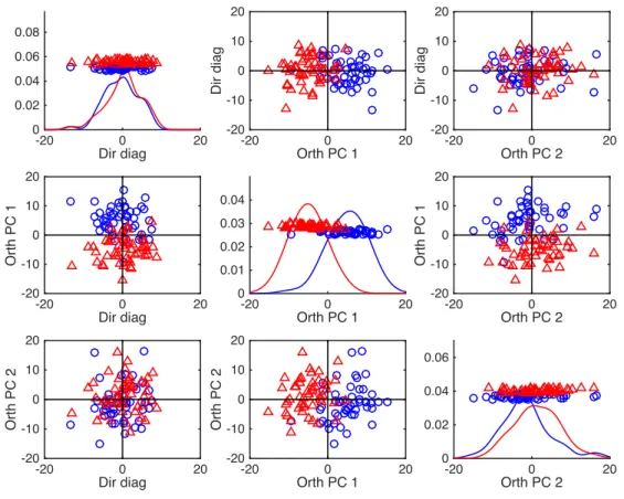
3.5 Projections of Two-class Auto-Regressive data onto the diagonal

direction and first 2 orthogonal PC directions . . . 39

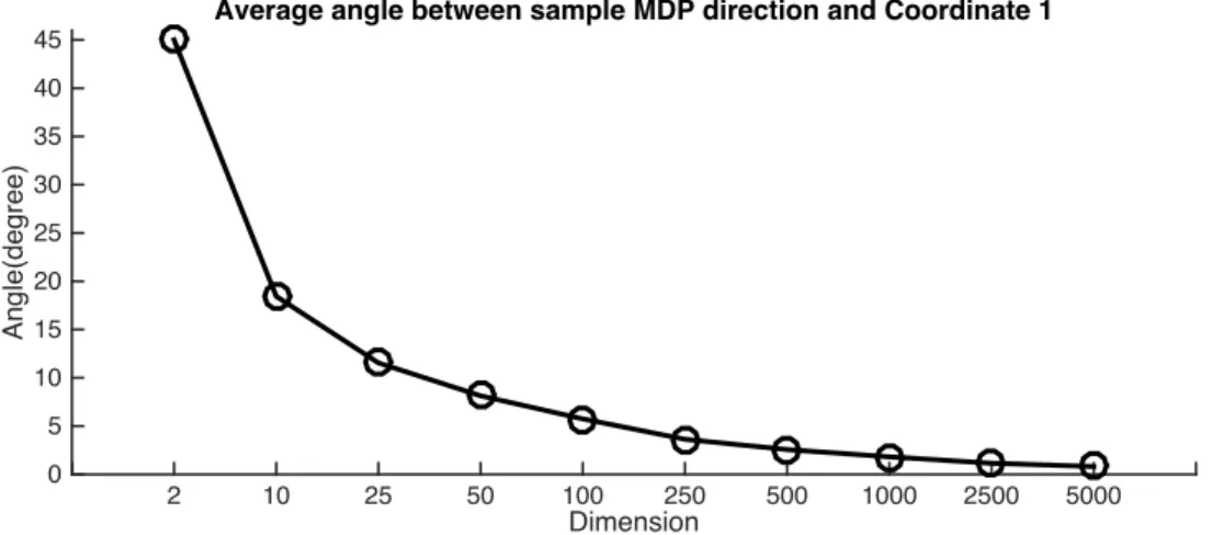
3.6 Monte Carlo average angle between the MDP normal vector and

e

for Two-class Auto-Regressive data structure . . . 48

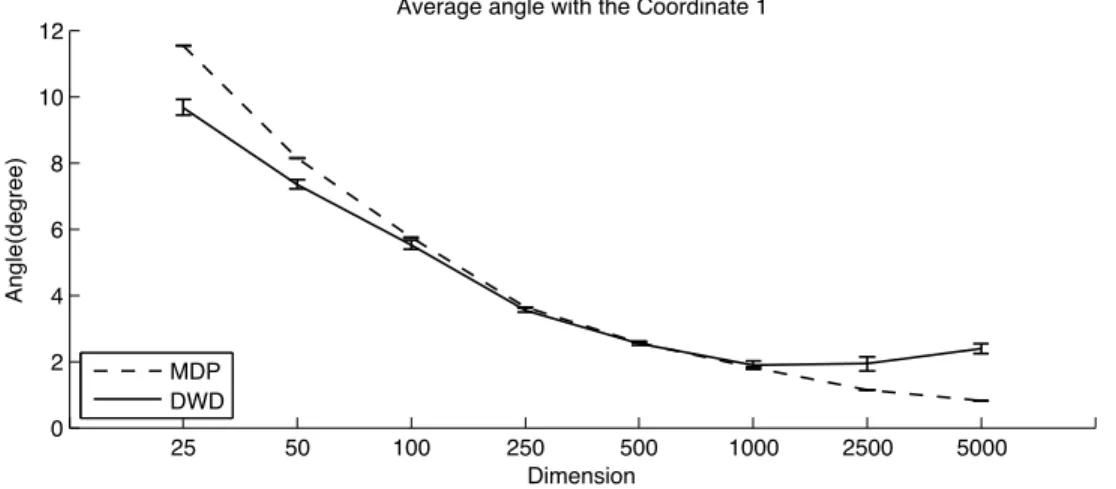
3.7 Monte Carlo average angle between MDP (and DWD) normal

vector and

e

for Two-class Auto-Regressive data structure . . . 57

4.1 Examples showing the disadvantages of the second version of

the CSPCA optimization criterion . . . 74

4.2 Examples showing the disadvantages of the third version of the

CSPCA optimization criterion . . . 76

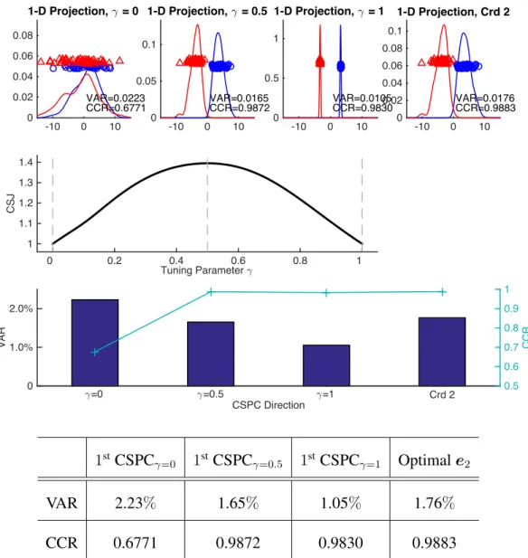
4.3 One-dimensional projections onto CSPC directions corresponding

to three different values of

. . . 82

4.4 Comparison of the data representation and classification

performances for a series CSPC directions . . . 85

4.5 Projections of the Two-class Auto-Regressive data onto the first

3 sample PC directions . . . 88

4.6 Projections of the Two-class Auto-Regressive data onto the Bayes

optimal direction and first 2 orthogonal PC directions . . . 90

4.7 Projections of the Two-class Auto-Regressive data onto the MDP

4.8 The curve of CSJ as a function of of the Two-class

Auto-Regressive data . . . 92

4.9 One-dimensional projections onto CSPC directions corresponding

to three different values of

. . . 93

4.10 Projections onto two CSPC directions where is near

0

of the

Two-class Auto-Regressive data . . . 95

4.11 Projections onto two CSPC directions where is near

1

of the

Two-class Auto-Regressive data . . . 96

4.12 Projections of the Two-class Auto-Regressive data onto the first

3 CSPC directions . . . 97

4.13 Projections of the Two-class Auto-Regressive data onto the FLD

normal vector and first 2 orthogonal PC directions . . . 99

4.14 Projections of the Two-class Auto-Regressive data onto the DWD

normal vector and first 2 orthogonal PC directions . . . 100

4.15 Projections of the Two-class Auto-Regressive data onto the SVM

normal vector and first 2 orthogonal PC directions . . . 102

4.16 Monte Carlo average performances of different methods of the

Two-class Auto-Regressive data . . . 103

4.17 Monte Carlo average percentage of VAR and log error rate for

different methods of the Two-class Auto-Regressive data . . . 105

4.18 Projections of the first simulated example onto the first 3 sample

PC directions . . . 108

4.19 Projections of the first simulated example onto the first 4 sample

PC directions . . . 109

4.20 The curve of CSJ as a function of of the first simulated example . . . 110

4.21 Projections of the first simulated example onto the first 4 CSPC

directions . . . 111

4.22 Comparison of the absolute value of the loadings for PCA and

CSPCA of the first simulated example . . . 112

4.23 Projections of the first simulated example onto the DWD normal

vector and first 3 orthogonal PC directions . . . 114

4.24 Projections of the first simulated example onto the FLD normal

vector and first 3 orthogonal PC directions . . . 117

4.26 Projections of the first simulated example onto the SVM normal

vector and first 3 orthogonal PC directions . . . 118

4.27 Monte Carlo average performances of different methods of the

first simulated example . . . 120

4.28 Projections of the Thyroid cancer data onto the first 3 sample PC

directions . . . 123

4.29 The curve of CSJ as a function of of the Thyroid cancer data . . . 124

4.30 Projections of the Thyroid cancer data onto the first 3 CSPC

directions . . . 125

4.31 Projections of the Thyroid cancer data onto the DWD normal

vector and first 2 orthogonal PC directions . . . 126

4.32 Projections of the Thyroid cancer data onto the FLD normal

vector and first 2 orthogonal PC directions . . . 127

4.33 Projections of the Thyroid cancer data onto the MDP normal

vector and first 2 orthogonal PC directions . . . 128

4.34 Projections of the Thyroid cancer data onto the SVM normal

vector and first 2 orthogonal PC directions . . . 129

4.35 Monte Carlo average performances of different methods of the

Thyroid cancer data . . . 130

5.1 Relationship between HDLSS asymptotic properties of MDP

normal vector for different choices of

a

and

max (

b, c

)

. . . 160

5.2 Graphical illustration of the asymptotic properties of the

1

PC

direction under the population model (5.3) and (5.4) . . . 162

5.3 Simulation illustration of MDP HDLSS asymptotic theorem . . . 165

5.4 MDP HDLSS asymptotic projection of Case 2 . . . 177

5.5 MDP HDLSS asymptotic projection of Case 3a . . . 179

5.6 MDP HDLSS asymptotic projection of Case 3b . . . 181

5.7 MDP HDLSS asymptotic projection of Case 4a . . . 183

5.8 MDP HDLSS asymptotic projection of Case 4b . . . 185

5.10 MDP HDLSS asymptotic projection of Case 5b . . . 189

5.11 Relationship between HDLSS asymptotic properties of CSPC

direction(s) for different choices of

max (

a, b

)

and

c

. . . 202

5.12 Simulation illustration of CSPCA HDLSS asymptotic theorem . . . 204

6.1 MDP null space graphical illustration . . . 228

6.2 Simulated data illustrates the projection of the 3-class data onto

the MMDP subspace proposed by Ahn and Marron (2010) . . . 231

6.3 Simulated data illustrates the projection of the 3-class data onto

the MMDP subspace using the new null space approach . . . 232

6.4 Simulated data illustrates the projection of the 3-class data onto

the MMDP subspace after rotation . . . 233

6.5 Graphically illustration of the underlying distribution of the

simulated example for the MCSP . . . 236

6.6 Projections of the simulated data for MCSP onto the first 3 PC

directions . . . 237

6.7 Projections of the simulated data for MCSP onto the 4

_{, 5}

_and

6

_{directions . . . 238}

6.8 Projections of the simulated data for MCSP on the Multi-class MDP

subspace . . . 239

6.9 The curve of MCSJ as a function of of the simulated data . . . 240

6.10 Projections of the simulated data for MCSP onto the first 4 MCSP

directions . . . 241

6.11 First 6 PC and MCSP loading vectors comparison of the simulated

data for MCSP . . . 242

6.12 Projections of the Thyroid cancer data (3 classes) onto the first 3

PC directions . . . 246

6.13 Projections of the Thyroid cancer data (3 classes) onto the

Multi-class MDP subspace . . . 247

6.14 The curve of MCSJ as a function of for the Thyroid cancer data

(3 classes) . . . 248

6.15 Projections of the Thyroid cancer data (3 classes) onto the first 3

6.16 The PCA and MCSP 1-dimensional projections comparison of the

Thyroid cancer data (3 classes) . . . 250

6.17 The PCA and MCSP 2-dimensional projections comparison of the

Thyroid cancer data (3 classes) . . . 251

6.18 SWISS permutation test of the Thyroid cancer data (3 classes) . . . 253

6.19 SWISS permutation test of the Thyroid cancer data (3 classes) for

N components . . . 255

6.20 Projections of the testing Thyroid cancer data (3 classes) onto the

first 3 training PC directions . . . 256

6.21 Projections of the testing Thyroid cancer data (3 classes) onto the

first 3 training MCSP directions . . . 257

6.22 Projections of the Thyroid cancer data (4 classes) onto the first 4

PC directions . . . 259

6.23 Projections of the Thyroid cancer data (4 classes) onto the

Multi-class MDP subspace . . . 260

6.24 The curve of MCSJ as a function of of the Thyroid cancer data

(4 classes) . . . 261

6.25 Projections of the Thyroid cancer data (4 classes) onto the first 4

MCSP directions . . . 262

6.26 The PCA and MCSP 2-dimensional projections comparison of the

Thyroid cancer data (4 classes) . . . 263

6.27 SWISS permutation test of the Thyroid cancer data (4 classes) for

N components . . . 265

6.28 Projections of the testing Thyroid cancer data (4 classes) onto the

first 4 training PC directions . . . 266

6.29 Projections of the testing Thyroid cancer data (4 classes) onto the

CHAPTER 1: INTRODUCTION

In the past few decades, the scope of statistics has been broadened to include exploratory

analysis and data visualization - going beyond the usually taught standard paradigms of

esti-mation and testing, to look for patterns in data beyond initial expectations (see Tukey (1970),

Tukey (1977), Velleman and Hoaglin (1981), Chambers (1983), Buja et al. (1996) and

Gel-man (2004) for detailed discussions).

Exploratory Data Analysis

, an approach to analyzing

datasets to summarize their main characteristics, uncover underlying structure and extract

important variables, often with visual methods is continuously developing. Exploratory

tech-niques for datasets in which a small number of variables are measured for a given set of

ob-jects are well developed. However, improvements in measurement, computation and

technol-ogy have produced complex datasets that require new exploratory techniques. Among them

the

High Dimension Low Sample Size

(

HDLSS

) data are becoming increasingly common in

various fields. These fields include genetic micro-arrays, medical imaging and chemometrics

in which hundreds or thousands of variables are measured for each object of interest (see

Hall et al. (2005)).

The technique of

Principal Components Analysis

(

PCA

), invented by Pearson (1901) and

named by Hotelling (1933), is a famous exploratory method which has been successfully

ap-plied in a variety of disciplines. However, PCA is driven entirely by variation of the dataset

not give effective data visualization. Therefore, the result is often difficult to interpret. Some

sparse PCA methods such as Zou et al. (2006) and Shen and Huang (2008) seek combinations

of few variables (modified PC directions with sparse loadings) to find informative structure

of high dimensional data. However, class labels are not considered in these methods. On the

other hand, linear classifiers such as

Fisher Linear Discrimination

(

FLD

),

Maximal Data

Pil-ing

(

MDP

),

Support Vector Machine

(

SVM

) and

Distance-Weighted Discrimination

(

DWD

)

focus on finding the best hyperplane to separate different types of data. The normal vector is

the direction perpendicular to the separating hyperplane. The projection of the dataset onto

the normal vector can give good visualization of the separation. As the dimension get higher,

some linear discrimination methods are going to overfit the data. Therefore they cannot give

effective data visualization. Some sparse regression methods such as Tibshirani (1996), Fan

and Li (2001), and Zou (2006) select subset of variables to provide better prediction.

How-ever, within-class variations are not targeted by these methods. In a variety of applications,

the within-class variations are important for visualization. For example, suppose we have a

dataset consisting of gene expressions of two types of cancer cells. In each type, men and

women may have different gene profiles. Although linear classifiers can separate the two

cancer types very well, from the 1-dimensional projection onto the normal vector, we may

not be able to visualize the different variations of men and women within each type. Hence

we develop a new statistical method that seeks direction vectors which capture not only the

variations but also the predefined class label information of the dataset. This method

com-bines the advantages of PCA and linear classifiers and compensates their disadvantages at the

can provide very informative data visualization.

The rest of this dissertation is laid out as follows. In Chapter 2 and Chapter 3 we give

the background of the

Object Oriented Data Analysis

(

OODA

) (Marron and Alonso (2014))

including exploratory methods, discrimination methods and some mathematical statistical

properties. In Subsection 3.3.5, we study the geometric representation of an interesting

dataset with strongly auto-regressive errors under the HDLSS setting and understand why the

MDP, proposed by Ahn et al. (2007), is the best in terms of classification compared with

sev-eral commonly used discrimination methods. In Chapter 4, we introduce the

Class-Sensitive

Principal Components Analysis

(

CSPCA

), which is a compromise of PCA and MDP, that

seeks new direction vectors for better Class-Sensitive visualization. Section 4.1 describes the

CSPCA method, 4.3 describes the criterion of choosing the tuning parameter and gives

ap-plications on simulated examples and a real dataset, and 4.5 describes a variation of CSPCA

and its relationship to the

Continuum Canonical Correlation

(

CCC

), proposed by Lee (2007).

In Chapter 5, we investigate the asymptotic behavior of MDP normal vector and CSPC

di-rections under the HDLSS setting. In Chapter 6 we introduce the Multi-class version of

CHAPTER 2: EXPLORATORY METHODS

In this chapter we review three commonly used exploratory methods for Objected

Ori-ented Data Analysis (OODA) (see Marron and Alonso (2014) and Wang and Marron (2007)

for detailed discussions). These methods can be utilized to explore the structure and uncover

patterns within a single multivariate dataset or discover relationship among multiple datasets.

In particular, we review the

Singular Value Decomposition

(

SVD

) in Section 2.1, Principal

Components Analysis (PCA) in Section 2.2 and

Canonical Correlation Analysis

(

CCA

) in

Section 2.3 respectively.

2.1 Singular Value Decomposition

The Singular Value Decomposition (SVD) is a factorization of a real-valued or

complex-valued matrix into a product of a diagonal matrix and two orthogonal matrices. Formally, let

X

be a real-valued matrix of dimension

d

_⇥

n

:

d

variables measured on

n

samples. Then

there exists a factorization of the form

X

=

U

⇤

V

,

(2.1)

where

U

is a

d

⇥

d

unitary matrix,

⇤

is a

d

⇥

n

diagonal matrix with non-negative numbers

on the diagonal, and

V

is an

n

_⇥

n

unitary matrix. The diagonal entries

of

⇤

are the

left-singular vectors and right-left-singular vectors of

X

respectively. The singular values are usually

listed in descending order, giving the SVD a unique representation if all the singular values

are different. The number of non-zero singular values of

X

(found on the diagonal entries of

⇤

) is equal to the rank of

X

. Therefore, the number of non-zero singular values is less than

or equal to

min (

d, n

)

.

The SVD has a variety of applications, one of the most important is the low-rank matrix

approximation. Consider solving the problem of approximating a matrix

X

by another same

size matrix

_X

ˆ

_{, which has a specific rank}

_r

_{. In this case the approximation is based on}

minimizing the

Frobenius norm

(

k

X

k

=

qPd

Pn

x

ij

) of the difference between

X

and

_X

ˆ

_:

ˆ

X

= ˆ

U

⇤

ˆ

V

ˆ

,

(2.2)

where

_⇤

ˆ

_{is the same as}

_⇤

_{except that it contains only the}

_r

_{largest singular values,}

_U

ˆ

_{is a}

d

⇥

r

matrix of the first

r

columns of

U

, and

V

ˆ

is an

n

⇥

r

matrix of the first

r

columns of

V

. This is known as the

Eckart-Young

Theorem (see Eckart and Young (1936)).

2.2 Principal Components Analysis

The technique of Principal Components Analysis (PCA) was invented by Karl Pearson

(see Pearson (1901) and Jolliffe (2005) for detailed discussions). The principal components

transformation of a centered data matrix (row means have been subtracted) can be associated

X

is centered so that each row of

X

has mean 0. Then the first

r

principal components are

computed by the rank

r

SVD approximation of

X

as (2.1), where the

d

_⇥

r

matrix

U

ˆ

gives the

first

r

principal component loading vectors for each variable and the

r

⇥

n

matrix

S

ˆ

= ˆ

⇤

V

ˆ

gives the first

r

principal component scores for each sample. Therefore the approximation

ˆ

X

can be written as

ˆ

X

= ˆ

U

S

ˆ

.

The scores

_S

ˆ

_{reveal the structure in the samples that represent the amount of variability in the}

data matrix

X

and the loading vectors

U

ˆ

define the size of the contribution of each original

variable to the principal components.

Rather than being merely associated with SVD, PCA also has an important geometric

interpretation in terms of variation. Since the row centered

d

⇥

n

data matrix

X

can be

decomposed as (2.1). The projections of

X

on

U

and

V

are:

Proj

=

U

X

=

U

U

⇤

V

=

⇤

V

,

Proj

=

XV

=

U

⇤

V

V

=

U

⇤.

The first column vector of

U

, denoted by

u

, satisfies

u

= arg max

Var

u

X

= arg max

u

X

u

X

The Equation (2.3) can be rephrased as

u

= arg max

u

T SS

u

(2.4)

where TSS refers to the Total Sum of Squares (

T SS

=

XX

).

After subtracting the first

k

1

principal components from

X

:

˜

X

=

X

k 1

X

s=1

usu

X

then the

k

column vector of

U

, denoted by

uk

, satisfies

uk

= arg max

Var

⇣

u

Xk

˜

⌘

.

Therefore

u

is the direction in the

d

-dimensional sample space maximizing the variation

of the projected samples in

X

, and

ui

, for all

i

= 2

,

3

, . . .

is the direction maximizing the

variation while orthogonal to the first

i

1

directions. Hence the scores

S

of the first

r

principal components are given as

S

=

U

X

=

0

B

B

B

B

B

B

@

u

1

X

...

u

X

1

C

C

C

C

C

C

A

.

With this geometric interpretation, visualization of the first few principal component

vantage points, in terms of variation explained.

The principal components can not only be interpreted as maximizing the projected

vari-ation, but also be interpreted as minimizing the projection Residual Sum of Squares (RSS).

To see why this is, let

u

2

R

_{be a vector with norm 1. Then}

_uu

_X

_{is the projection of the}

data matrix

X

onto

u

. We minimize the projection RSS over

u

:

RSS

(u) =

_k

X

uu

_X

_k

₌

n

X

i=1

k

x

uu

x

k

(2.5)

where

xi

for all

i

= 1

, . . . , n

is the

i

column of the matrix

X

. After some algebra we have

RSS

(u) =

X

i=1

xix

X

i=1

x

uu

xi

.

(2.6)

The first term doesn’t depend on

u

, so it doesn’t appear in the minimization of the residual

sum of squares. To make RSS small, what we must do is make the second term big, i.e., we

want to maximize

n

X

i=1

x

uu

xi

=

u

X

u

X

=

u

XX

u

.

(2.7)

Therefore the optimal solution of minimizing RSS

(u)

is the 1

principal component

direc-tion of data matrix

X

. In general it is useful to project onto multiple vectors, say

r

vectors,

which are orthogonal and have norm 1. Then the residual sum of squares is

RSS

(u

ur) =

_k

X

X

Similar algebra as in (2.5), (2.6) and (2.7) gives that the optimal solutions are the first

r

principal components of the data matrix

X

. In other words, the RSS of

X

projected onto

r

orthonormal vectors is minimized by the first

r

principal components.

2.3 Canonical Correlation Analysis

Canonical Correlation Analysis (CCA) (first introduced by Hotelling (1936)) is one of

the principle tools in multivariate statistics for studying the relationship between two sets of

multivariate data. CCA seeks two vectors such that the correlation between the projections

of variables onto these vectors are maximized.

2.3.1 Review of Canonical Correlation Analysis

Formally, let

X

and

Y

be two centered (row means have been subtracted) matrices of

dimension

d

⇥

n

and

d

⇥

n

respectively. Denote

u

and

v

as

d

⇥

1

and

d

⇥

1

vectors

respectively. The correlation between the two projections Proj

=

u

X

and Proj

=

v

Y

can be written as

⇢

=

p

Cov

(

Proj

,

Proj

)

Var

(

Proj

)

p

Var

(

Proj

)

=

u

T

_XY

_v

p

u

_XX

_u

p

_v

_{Y Y}

_v

.

Note that the correlation is scale invariant under affine transformation of both data matrices,

constraints

u

_XX

_u

₌

_v

_{Y Y}

_v

_{= 1}

_{. Then CCA is equivalent to the following:}

max

u,v

u

T

_XY

_v

_(2.8)

subject to

u

_XX

_u

₌

_v

_{Y Y}

_v

_{= 1}

_{. The corresponding Lagrange form is}

u

XY

v

2

u

T

_XX

u

1

2

v

T

_{Y Y}

v

1

.

Take the partial derivatives w.r.t.

u

and

v

, and setting the them equal to 0 gives the following

equations

XY

v

=

u

,

(2.9)

Y X

u

=

Y Y

v

.

(2.10)

Subtracting

u

times (2.9) from

v

times (2.10), we obtain

xuT

XX

u

v

Y Y

v

= 0

,

which implies

x

=

=

⇢.

Assuming

Y Y

is invertible we have

v

=

Y Y

T 1

_{Y X}

_u

Similarly assuming

XX

is invertible we have

u

=

XX

T 1

_XY

_v

⇢

.

(2.12)

Substituting (2.11) and (2.12) into equations (2.9) and (2.10) and rearranging terms gives the

following generalized eigen-analysis

XY

Y Y

Y X

u

=

⇢

XX

u

,

(2.13)

Y X

XX

XY

v

=

⇢

Y Y

v

.

(2.14)

The solution is therefore:

•

u

is an eigenvector of

XX

XY

Y Y

Y X

if

XX

is invertible,

•

v

is an eigenvector of

Y Y

Y X

XX

XY

if

Y Y

is invertible.

Therefore the eigenvectors

u

and

v

corresponding to the largest eigenvalues of

XX

XY

Y Y

Y X

and

Y Y

Y X

XX

XY

respectively are the first pair of canonical direction vectors. Then the empirical correlation

between projections

u

vari-2.3.2 The relationship between

⇢

and the size of dataset

Suppose we have two data matrices

X

and

Y

from probability distributions that are

ab-solutely continuous with respect to Lebesgue measure. We have the following theorem which

claims that, with probability

1

, there exist a pair of direction vectors such that the correlation

between the projections of

X

and

Y

is 1 if the dimension of the vertical concatenation of the

two data matrices is greater than or equal to the samples size.

Theorem 1.

Suppose we have two data matrices

X

and

Y

from probability distributions

that are absolutely continuous with respect to Lebesgue measure. Their sizes are

d

⇥

n

and

d

⇥

n

respectively. Denote

d

=

d

+

d

as the dimension of the vertical concatenation of

X

and

Y

. If

d

n, then with probability 1, there exist vectors

a

₂

R

and

b

2

R

such

that the empirical correlation between the projections Proj

=

a

_X

_{and Proj}

b

=

b

Y

is 1.

Define

Z

= (X;

Y

)

to be the

d

_⇥

n

vertical concatenation of

X

and

Y

. Since the mean

of

Z

for each row is 0 and

d

n

, we know that rank

(Z) =

r

_

n

1

. Thus

Z

can be

decomposed by SVD as

Z

=

r

X

i=1

iuivT_i

where

ui

2

R

_,

_vi

₂

_R

_,

_u

i

ui

=

v

vi

= 1

, for all

i

= 1

, . . . , n

and

u

uj

=

v

vj

= 0

, for

all

i

₆

=

j

.

It naturally follows that

ZZ

=

X

i=1 2

And it is easy to see that, given any pair

a

2

R

and

_b

2

R

, we have

a

XY

b

=

1

2

2

6

6

4

✓

a

_b

◆

ZZ

0

B

B

@

a

b

1

C

C

A

a

XX

a

b

Y Y

b

3

7

7

5

(2.15)

and

✓

a

_b

◆

ZZ

0

B

B

@

a

b

1

C

C

A

=

X

✓

a

_b

◆

ui

u

0

B

B

@

a

b

1

C

C

A

.

(2.16)

Solving for

a

and

b

to make (2.16) be 0, we have

✓

a

_b

◆

ui

= 0

,

for all

i

= 1

, . . . , r

(2.17)

because

i

>

0

and

✓

a

_b

◆

uiu

0

B

B

@

a

b

1

C

C

A

0

, for all

i

= 1

, . . . , r

. We write

ui

as

0

B

B

@

ui,X

ui,Y

1

C

C

A

, where

ui,X

is a vector which consists of the first

d

elements of

ui

and

ui,Y

is a

vector which consists of the remaining

d

elements of

ui

. Then (2.17) can be rephrased as

a

ui,X

=

b

ui,Y

,

for all

i

= 1

, . . . , r.

(2.18)

Since

Z

=

X

=

0

B

B

@

Pr

i=1 iui,X

v

Pr

iui,Y

v

1

C

C

A

and

Z

=

we know that

X

=

r

X

i=1

iui,X

v

,

Y

=

r

X

i=1

iui,Y

v

.

Equations (2.18) imply that

a

XX

a

=

b

Y Y

b

.

(2.19)

Then equations (2.15) and (2.19) together imply that

⇢

=

a

T

_XY

_b

p

a

_XX

_a

p

_b

_{Y Y}

_b

= 1

.

Because

⇢

is scale invariant under affine transformations of

a

and

b

, we can set another

constraint

a

XX

a

=

C,

where

C

is a positive constant to make the solution unique. Therefore we have

a

XX

a

=

C

(2.20)

a

ui,X

b

ui,Y

= 0

for all

i

= 1

, . . . , r

(2.21)

1. If

d



n

1

, there may not exist any vectors

a

and

b

such that

⇢

= 1

.

2. If

d

=

n

, with probability 1, there exist at least one pair of vectors

a

and

b

such that

⇢

= 1

.

3. If

d

n

+ 1

, with probability 1, there exist many pairs of vectors

a

and

b

such that

⇢

= 1

.

Next we use simulated examples to illustrate the above conclusions. In each panel of

Figure 2.1, two datasets

X

and

Y

follow two uncorrelated Gaussian distributions. For each

distribution we simulated

n

= 50

samples. The projections onto the first pair of CCA

direc-tion vectors are plotted in Figure 2.1.

CC sample scores X

-5 0 5

CC sample scores Y

-5 0 5

;=0.202 d_X=2, d_Y=2, n=50

CC sample scores X

-5 0 5

CC sample scores Y

-5 0 5

;=0.835

d_X=15, d_Y=15, n=50

CC sample scores X

-5 0 5

CC sample scores Y

-5 0 5

;=1

d_X=25, d_Y=25, n=50

Figure 2.1: The first pair of CCA scores forX andY. The left two panels show that whend < n 1,

the empirical correlation between CCA scores is less than1. The right panel shows that

when d = n, the empirical correlation between CCA scores is 1. These three panels

illustrate the tendency of CCA to overfit asd_{! 1}.

In the left two panels of Figure 2.1, the dimension

d

is less than the sample size

n

. We

can see that the projections do not lie along the 45

_{line perfectly. Therefore the correlation}

perfectly. Therefore the correlation is

1

. These three panels illustrate the tendency of CCA to

overfit as

d

_{! 1}

. If the matrix

Y

is a class indicator vector, we have the following corollary.

Corollary 1.

Suppose a

d

⇥

n

data matrix

X

is from a probability distribution that is

absolutely continuous with respect to Lebesgue measure. Further assume that

_Y

˜

_{is a}

₁

_⇥

_n

class indicator vector

˜

Y

= (˜

y1, . . . ,

y

˜

,

(2.22)

where

y

˜

2

{

1

,

+1

}

for all

i

= 1

, . . . , n. We denote

Y

as the centered version of

Y

˜

, then

the dimension of matrix

Z

= (X;

Y

)

is

d

+ 1

. Suppose rank

(X

) = min (

d

, n

1)

, then

we have the following conclusions

1. If

d



n

2

, there do not exist any vectors

a

and

b

such that

⇢

= 1

. In other words,

⇢

is always less than 1.

2. If

d

n

1

, with probability 1, there exist at least one pair of vectors

a

and

b

such

that

⇢

= 1

.

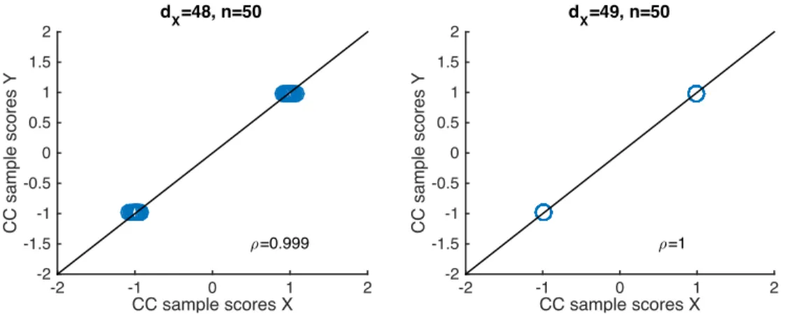
Again, we will use simulated examples to illustrate the above conclusions. The

CC sample scores X

-2 -1 0 1 2

CC sample scores Y

-2 -1.5 -1 -0.5 0 0.5 1 1.5 2

;=0.999 d_X=48, n=50

CC sample scores X

-2 -1 0 1 2

CC sample scores Y

-2 -1.5 -1 -0.5 0 0.5 1 1.5 2

;=1 d_X=49, n=50

Figure 2.2: The first pair of CCA directions forX andY, whereY is a1⇥nclass indicator vector. The left panel shows whendX = n 2, the empirical correlation between CCA scores

is less than 1. The right panel shows whendX =n 1, the projection of all points onto

the CCA directions are piled at two distinct values. Therefore the empirical correlation between CCA scores is perfect as 1.

In each panel of Figure 2.2,

Y

is a class indicator vector defined as (2.22), data matrix

X

consists of

n

= 50

d

-dimensional samples simulated from a Gaussian distribution. In the

left panel, the dimension of

X

is

d

= 48



n

2

. We can see that the projections do not

lie along the 45

_{line perfectly. Therefore the correlation is less than 1. In the right panel,}

the dimension is

d

= 49

n

1

. We can see that the projections lie along the 45

line

perfectly. Therefore the correlation is perfect as 1. In addition, if we project the data onto the

first CCA direction of

X

, all data points will pile at only two distinct values. This interesting

CHAPTER 3: LINEAR DISCRIMINATION METHODS

In this chapter we first review four linear methods for two-class discrimination. The goal

of discrimination is to find a rule for assigning the labels

+1

or

1

to new data vectors,

depending on whether the vectors are “more like class

+1

” or “more like class

1

”. In

particular, we review the Fisher Linear Discrimination (FLD) in Section 3.1, Support Vector

Machine (SVM) in Section 3.2, Maximal Data Piling (MDP) in Section 3.3 and Distance

Weighted Discrimination (DWD) in Section 3.4. In Subsection 3.3.5, we study the geometric

representation of an interesting dataset with strongly auto-regressive errors under the HDLSS

setting and understand why the MDP is the best in terms of classification compared with

several other commonly used linear discrimination methods. Then we review a quantitative

measurement called Standardized WithIn class Sum of Squares (SWISS) for quantifying how

well a data clusters into predefined classes in Section 3.5. Within this section, we will also

discuss the relationship of SWISS with MDP.

3.1 Fisher Linear Discrimination

As we reviewed in Section 2.2, PCA is an exploratory technique which does not use

the predefined class label information. We refer to this kind of technique as

unsupervised

techniques

. How can the class label information be used in finding information projections?

sification in this 1-dimensional space.

Formally, we use a

d

_⇥

n

matrix

X

= (x

xn)

to denote our centered (where row

means have been subtracted) dataset. Let

X

and

X

denote the collection of samples

xi

which belong to Class

+1

and Class

1

respectively. We use

n+1

and

n

to denote the

number of samples of each class. Besides, we let

_X

˜

_and

_X

˜

_{denote the centered versions}

of

X

and

X

respectively.

Suppose the two classes of samples have sample means

x

¯

and

x

¯

and sample

covari-ances matrices

S

and

S

respectively. The normal vector perpendicular to the

discrimi-nant hyperplane is defined as the solution

w

2

R

_{found by maximizing}

J

(w) =

w

T

_BSS

_w

w

_{W SS}

_w

(3.1)

subject to

w

_w

_{= 1}

_{, where BSS is the “Between-class Sum of Squares” defined as}

BSS

=

XX

X

˜

X

˜

T

+1

X

˜

X

˜

T

1

,

and WSS is the “Within-class Sum of Squares” defined as

W SS

= ˜

X

X

˜

T

+1

+ ˜

X

X

˜

T

1

.

Maximizing

J

(w)

yields a closed form of optimal normal vector, i.e., the FLD normal vector

w

=

W SS

1

_(¯

_x

If WSS is not invertible, then we use the Moore-Penrose pseudoinverse (see Chapter 1 of

Ben-Israel and Greville (2003) for detailed discussions). Thus we have obtained

w

for FLD

- the linear function yielding the maximum ratio of BSS to WSS. The classification has been

converted from a

d

-dimensional problem to a more manageable 1-dimensional one.

Similar to Canonical Correlation Analysis reviewed in Subsection 2.3.1, solving the

op-timization problem (3.1) yields the following generalized eigen-analysis

BSS

w

=

W SS

w

,

(3.3)

and the FLD normal vector is the eigenvector corresponding to the largest eigenvalue. Since

matrix BSS is of rank 1, there is only 1 non-zero eigenvalue of this generalized eigen-analysis

(3.3). And the unit length eigenvector corresponding to this eigenvalue has the closed form

as (3.2).

3.2 Support Vector Machine

The Support Vector Machine (SVM) was first proposed by Cortes and Vapnik (1995). The

SVM constructs a hyperplane in a high-dimensional space, which can be used for

classifica-tion, regression, or other tasks. Intuitively, a good separation is achieved by the hyperplane

that has the largest distance to the nearest training data point of any class. Again, let our

training dataset be the same as in Section 3.1. Defined a hyperplane by

where

w

is a unit vector. For the moment we assume that the classes are separable, i.e., we

can find a function

f

(x) =

x

_w

₊

_with

_y

i

f

(xi)

>

0

for all

i

= 1

, . . . , n

. The key idea

behind SVM is to find

w

and to keep the data in the same class all on the same side of, and

also as far as possible from, the separating hyperplane. This is quantified using a maximum

optimization formulation, focusing only on the training data points closest to the separating

hyperplane, called

support vectors

. The optimization problem

max

w,

M

(3.4)

subject to

y

x

w

+

M

for all

i

= 1

, . . . , n

and

w

w

= 1

captures this concept. This

problem can be more conveniently rephrased as

min

w,

k

w

k

(3.5)

subject to

y

x

w

+

1

for all

i

= 1

, . . . , n

, which is equivalent to

min

w,

1

2

w

T

_w

_(3.6)

subject to

y

x

w

+

1

for all

i

= 1

, . . . , n

where we have dropped the norm constraint

on

w

. Note that

M

= 1

/

k

w

k

. Equation (3.6) is the usual way of writing the support vector

criterion for separated data.

Suppose now that the classes are no longer separable, i.e., they overlap in feature space.

as

y

x

w

+

M

(1

⇠

)

,

for all

i

= 1

, . . . , n

,

⇠

0

,

Pn

⇠



C

,

C

is a constant. The value

⇠

is the proportional

amount by which the prediction

f

(x

) =

x

w

+

is on the wrong side of its margin. Hence

by bounding the sum

Pn

⇠

, we bound the total proportional amount by which predictions

fall on the wrong side of their margin. Then the optimization problem is

min

1

2

w

T

_w

subject to

y

x

w

+

1

⇠

⇠

0

,

X

i=1

⇠



C

for all

i

= 1

, . . . , n

, which can be rephrased as

min

1

2

w

T

_w

₊

_C

₁

n

⇠

(3.7)

subject to

y

x

w

+

1

⇠

for all

i

= 1

, . . . , n

, where

1n

= (1

, . . . ,

1)

and

C

is a positive penalty parameter. In the

rest of this article we use Gunn’s recommendation of

C

= 1000

for SVM. This is the usual

way the SVM is defined for the non-separable case. By the nature of the criterion (3.7), we

see that points inside their class boundary do not play a role in shaping the boundary. More

details of SVM including the computation and examples can be found in Vapnik (2000);

Vapnik and Kotz (2006) , Burges (1998), Cristianini and Shawe-Taylor (2000), Schlkopf and

Smola (2001) and Hastie et al. (2013).

3.3 Maximal Data Piling

In two-class discrimination when the dimension is larger than the sample size, there exist

direction vectors onto which the data project to only two distinct values, one for each class.

The Maximal Data Piling (MDP) direction for discrimination was proposed by Ahn and

Marron (2010). Why it is called maximal data piling direction vector is because the data

are piled on two points while maximizing the distance in between. We assume that the

dimension

d

satisfies

d

n

1

, where

n

is the sample size. We also assume that the data are

not degenerate, in the sense of generating a subspace of dimension

n

. Data piling was first

discussed in Marron et al. (2007). They observed that the SVM classifier yielded substantial

data piling when it was applied to HDLSS data. MDP can be regarded as an extreme version

3.3.1 Review of Maximal Data Piling

We use the same notations as in Section 3.1. In addition, we use

_X

˜

₌

⇣

_X

˜

_X

˜

⌘

_to

denote the horizontal concatenation of the two centered matrices of the two classes.

The MDP normal vector is defined as the solution

w

2

R

_{found by solving the}

opti-mization problem

max

⇥

w

(¯

x

x

¯

)

⇤

(3.8)

subject to

w

_w

_{= 1}

_and

_X

˜

_w

_{= 0}

_{. This optimization problem can be interpreted as}

maximizing the squared difference between the projected class means while insisting that the

projection of each class point onto the unit direction vector is the same as its class mean.

There are some insightful optimization problem that are equivalent to (3.8). The MDP

normal vector

w

₂

R

_{can be found by solving the problem of maximizing}

J

(w) =

w

T

_BSS

_w

w

_{T SS}

_w

,

(3.9)

subject to

w

_w

_{= 1}

_{, where TSS is the “Total Sum of Squares” defined as}

T SS

=

XX

.

We can see that the above optimization problem is a simple replacement of the Within-class

Sum of Squares WSS in FLD optimization problem (3.1) by the Total Sum of Squares TSS.

Why does this make sense? It says that a good solution is one where the class means are

section that when

d



n

2

, (3.9) is equivalent to FLD, which does not have the piling

property. When

d

n

1

, (3.9) yields complete data piling. The FLD is invariant under

affine transformation of data when

d



n

2

, but (3.9) is not. However, we can view MDP

as an appropriate high dimension, low sample size version of FLD in the sense that it yields

data projections with zero WSS and maximized BSS.

Similar to Equation (3.2), maximizing

J

(w)

in (3.9) yields a closed form of optimal

normal vector, i.e., the MDP normal vector

w

=

T SS

1

_(¯

_x

+1

x

¯

)

k

T SS

_(¯

_x

+1

x

¯

)

k

.

(3.10)

If TSS is not invertible, we use the Moore-Penrose pseudoinverse. Similarly, solving the

MDP optimization problem (3.9) yields the following generalized eigen-analysis

BSS

w

=

T SS

w

(3.11)

and the MDP normal vector is the eigenvector corresponding to the largest eigenvalue of

T SS

_BSS

_{. More detailed discussion and examples can be found in Ahn and Marron}

(2010).

3.3.2 Maximal Data Piling solved by Canonical Correlation Analysis

In this subsection, we derive the connection between MDP and CCA. From the

connec-tion we can see that the MDP normal vector is a special case of the canonical vector using

indicator vector

Y

to have the form

Y

= (

y1, . . . , y

,

(3.12)

such that

y

2

{

q

1 n·n+1

,

q

n·n 1

}

for

i

= 1

, . . . , n

. We assume that there are

n

y

s equal

to

q

n·n+1

and

n y

s equal to

q

n·n 1

. Therefore it naturally follows

n

=

n+1

+

n

.

The reason why we use this specific class indicator vector instead of the conventional one

(2.22) in Subsection 2.3.2 is because applying this class indicator vector (3.12) to the CCA

calculation will give us the same generalized eigen-analysis as (3.11).

First we have that

XY

=

r

n+1n

n

(¯

x

x

¯

)

.

With the fact

Y Y

= 1

and using the result (2.13) in Subsection 2.3.1

XY

Y Y

Y X

u

=

⇢

XX

u

we have

n+1n

n

(¯

x

x

¯

) (¯

x

x

¯

)

T

=

⇢

XX

u

.

After some easy algebra we have

This can be equivalently rewritten as

BSS

u

=

⇢

T SS

u

,

(3.13)

which is identical to the generalized eigen-analysis of MDP (3.11).

This relationship shows that the MDP normal vector is the canonical vector of the

ma-trix

X

when

Y

is a class indicator vector. Next we use equation (3.13) to help us better

understand the connection between MDP and FLD.

3.3.3 Relationship to Fisher Linear Discrimination

Ahn discovered the identity of MDP and FLD normal vectors under non-HDLSS settings,

i.e.

d



n

2

, from their closed form solutions given by (3.10) and (3.2) respectively

in her dissertation (see Subsection 3.3.2 of Ahn (2006)). However, we study this property

from another perspective using generalized eigen-analysis in this subsection. The following

theorem says the FLD and MDP normal vectors are equivalent up to a

±

sign under

non-HDLSS settings.

Theorem 2.

Let

wF LD

and

wM DP

be the FLD and MDP normal vectors of the same dataset.

If

d



n

2

and the data matrix

X

is full rank, i.e., rank

(X) =

d

, then

wF LD

and

wM DP

are equivalent up to a

_±

sign.

Proof.

It is easy to see that

Therefore the Equation (3.13) can be written as

1

⇢

BSS

u

=

⇢

W SS

u

.

(3.14)

From the assumptions we know rank

(X) =

d



n

2

, then by Corollary 1 we know

that the correlation follows

⇢

<

1

. Therefore Equation (3.14) can be written as

BSS

u

=

⇢

2

1

⇢

W SS

u

.

(3.15)

This is identical to the generalized eigen-analysis of FLD in Equation (3.3) but with

=

⇢

_/

₍₁

_⇢

₎

_{. This implies that when}

_d

X



n

2

, MDP is equivalent to FLD up to a

±

sign,

which does not have the piling property.

From Corollary 1 we also know that when

d

n

1

, i.e. under the HDLSS settings,

with probability

1

, there exist

u

2

R

and

_v

2

R

such that

_⇢

_{= 1}

. Therefore (3.14) is

invalid to be written as the form (3.15) because the denominator becomes

0

. When

⇢

= 1

,

the projections of

X

onto

u

and of

Y

onto

v

have perfect correlation (refer to the right panel

in Figure 2.2), which yields complete data piling. Thus we have

Corollary 2.

Suppose

X

is a

d

_⇥

n

data matrix from a probability distribution that is

abso-lutely continuous with respect to Lebesgue measure and

Y

is a

1

⇥

n

class indicator vector,

1. When

d

n

1

, with probability 1, there exists a canonical vector

u

of

X

which is