Spin-triplet supercurrent carried by quantum Hall edge states through a Josephson junction
J. A. M. van Ostaay, A. R. Akhmerov, and C. W. J. Beenakker
Instituut-Lorentz, Universiteit Leiden, P. O. Box 9506, 2300 RA Leiden, The Netherlands
(Received 4 March 2011; revised manuscript received 6 April 2011; published 31 May 2011) We show that a spin-polarized Landau level in a two-dimensional electron gas can carry a spin-triplet supercurrent between two spin-singlet superconductors. The supercurrent results from the interplay of Andreev reflection and Rashba spin-orbit coupling at the normal-superconductor (NS) interface. We contrast the current-phase relationship and the Fraunhofer oscillations of the spin-triplet and spin-singlet Josephson effect in the lowest Landau level and find qualitative differences.
DOI:10.1103/PhysRevB.83.195441 PACS number(s): 73.23.−b, 73.43.−f, 74.45.+c, 74.78.Na
I. INTRODUCTION
The coexistence of the quantum Hall effect with the superconducting proximity effect provides a unique opportu-nity to study the flow of supercurrent in chiral edge states. The usual quantum Hall edge states1 in a two-dimensional (2D) electron gas are created by the interplay of cyclotron motion and reflection from an electrostatic potential, propagating in a direction dictated by the cyclotron frequencyωc=eB/m. At the interface with a superconductor Andreev reflection from the pair potential takes over, converting electrons into holes.2 Since the sign of both the effective massmand chargeechange on Andreev reflection, the cyclotron rotation keeps the same direction for electrons and holes and the chirality of these Andreev edge states is preserved.3–6
While the superconducting proximity effect is short ranged in the direction perpendicular to the edge states, it is long ranged in the parallel direction. Indeed, a supercurrent can flow through a 2D electron gas even if the magnetic field is so strong that only a single Landau level is occupied, provided the spin splitting by the Zeeman effect is sufficiently small.7,8
Andreev reflection from a spin-singlet superconductor couples opposite spin bands, so spin polarization of the Landau level suppresses the supercurrent.9,10
Recent studies of ferromagnetic Josephson junctions have shown that a spin-triplet proximity effect (with electrons and holes from the same spin band) can be induced by a spin-singlet superconductor, if the spin is not conserved at the ferromagnet-superconductor interface.11–13 In the 2D
electron gas of a quantum well formed in a narrow band gap semiconductor, such as InAs or InSb, the Rashba effect is a significant source of spin-orbit coupling in quantum Hall edge states.14 When contacted with Nb electrodes, these structures show a strong proximity effect in the quantum Hall effect regime.15–17
In this article we investigate whether the spin-polarized lowest Landau level of a 2D electron gas can carry a spin-triplet supercurrent between two spin-singlet superconductors, as a consequence of the Rashba effect on Andreev edge states. We find that a long-range spin-triplet proximity effect does exist, with a critical current ∝(d/ lso)2, determined by the spin-orbit scattering lengthlso in the normal region and the distance d over which the electrostatic potential drops on entering the superconductor. It is a small effect, but the fact that it exists as a matter of principle opens up the possibility to optimize it.
We calculate the current-phase relationship (dependence of the supercurrent on the superconducting phase difference) and the Fraunhofer oscillations (dependence on the magnetic flux through the junction) of the spin-triplet Josephson effect and compare with the corresponding spin-singlet effect. Some of our spin-singlet results are known,7,8,18but some are new. In
particular, we find a complete suppression of the Fraunhofer oscillations in the spin-singlet case for a critical value of the widthWof the Josephson junction. (These spin-singlet results may be of interest also for graphene, which shows a strong proximity effect19without significant spin-orbit coupling.)
In Sec.IIwe formulate the problem of edge-state transport along a superconductor, in the form of an effective Hamiltonian in the lowest spin-split Landau level. The parameters entering into this Hamiltonian are derived from the Bogoliubov-De Gennes equation in the Appendix. The spin-triplet Josephson effect is analyzed in Secs.IIIandIVand compared with the spin-singlet counterpart in Sec.V. We conclude in Sec.VI.
II. SPIN-POLARIZED TRANSPORT ALONG A SUPERCONDUCTOR
A. NS interface
We consider the scattering by a superconductor (excitation gap0, Fermi energyEF,S0) of a single spin-polarized edge channel in a 2D electron gas in a perpendicular magnetic fieldB. The lowest Landau level at12hω¯ c±12gμBBis split by the Zeeman energygμBB, and spin polarization is ensured by taking the Fermi levelEF in the 2D gas in between the two spin-split levels (typicallyEF ≈12¯hωc).
The characteristic energy and length scales at the normal-superconductor (NS) interface are shown in Fig.1. On the superconducting side we have the coherence length ξ0 = ¯
hvF,S/0, and the Fermi wave length λF,S=2π/kF,S = πhv¯ F,S/EF,S. We require that ξ0 is small compared to the magnetic lengthlm=
√ ¯
h/eB, to ensure thatBis well below the upper critical field of the superconductor.
The electrostatic potential step at the NS interface extends over a distanced, which we assume to be intermediate between λF,Sandξ0. These length scales are therefore ordered as
λF,S d ξ0 lm. (2.1)
FIG. 1. (Color online) Schematic drawing of the energy scales and length scales at an NS interface. The electrostatic potential profile is shown as a blue solid curve, the Fermi level is a red dashed line, and the superconducting excitation gap is green dashed. The red solid lines indicate the spin-split lowest Landau level, with only a single spin band occupied (short black arrows).
suppressed even without spin polarization.) The step in the pair potential is also rounded, but this has no significant effect on Andreev reflection (since0EF,S).
On the normal side of the NS interface the Fermi wave length islm, so this is not an independent length scale. The spin-orbit scattering length and coupling energy are lso= ¯
h2/mα andE
so=mα2/h¯2, respectively, with α the Rashba coefficient. Typical values of these parameters (representative for InAs) arelso=100 nm,Eso =0.1 meV.
B. Edge-channel Hamiltonian
The wave function=(ψe,ψh) of the electron and hole excitations (both in the same spin band) is an eigenstate of the Bogoliubov-De Gennes Hamiltonian H with energy eigenvalueε(measured relative to the Fermi level). Electron-hole symmetry dictates that, if (ψe,ψh) is an eigenstate at energy ε, then (ψh∗,ψe∗) is an eigenstate at energy−ε. This requires
σxH∗σx= −H, (2.2)
where the Pauli matrix acts on the electron-hole degree of freedom.
At low excitation energies an effective Hamiltonian, con-taining only terms linear in momentum along the edge, is sufficient. The form of this effective Hamiltonian is fully constrained by the requirements of Hermiticity and electron-hole symmetry,
H= 1 2
{
vc,p−eA} {v,p} {v∗,p} {vc,p+eA}
. (2.3)
Heresand ˆsare coordinate and unit vector along the edge,p= −i∂/∂sis the canonical momentum, andA=Asˆis the vector potential in a gauge where it is parallel to the edge. (We set ¯
h≡1 in intermediate formulas and write+efor the electron charge.) The anti-commutator {a,b} =ab+ba ensures that His Hermitian even if the velocitiesvcandvdepend ons.
FIG. 2. (Color online) The dispersion relation of edge states along an NS interface in the lowest spin-polarized Landau level, for the electron-like mode (solid) and the holelike mode (dashed). The black curves are calculated in the Appendix from the Bogoliubov-De Gennes equation (forEF = 12hω¯ cgμBB,v/vc1,λ/ lm1). The red lines are the small-papproximation (2.6).
The gauge transformation →exp(iχ σz) transforms the Hamiltonian as follows,
H →eiχ σzH e−iχ σz
= 1 2
{vc,p−eA−χ} {|v|eiφ+2iχ,p} {|v|e−iφ−2iχ,p} {v
c,p+eA+χ}
, (2.4)
withχ=∂χ /∂sandv= |v|eiφ. We ensure thatvis real positive by chosing 2χ= −φ. The effective Hamiltonian then takes the form
H=(vc+vσx)p−evcAσz−12i(vc+v σx). (2.5)
C. Dispersion relation
Fors-independentA,vc, andv the momentump along the edge is conserved. The Hamiltonian (2.5) describes two chiral modes with the dispersion relation
ε=vcp±
(evcA)2+(vp)2 (2.6)
(see Fig. 2). At ε=0 the two modes have the same group velocityvgroup=dε/dp, given by
vgroup=vc−v2/vc. (2.7)
Let us express vc and v in terms of the characteristic parameters of the NS interface. As derived in the Appendix, the two velocitiesvcandvare given, up to numerical coefficients of order unity, by
vclmωc, v vcd
lso
. (2.8)
The velocityvcis the same as the cyclotron drift velocity in the lowest Landau level along a normal, not superconducting boundary, in the limit of a steep confining potential. The confinement by the superconductor is effectively in that limit because the penetration depth ξ0 of the edge state into the superconductor is less than its transverse extensionlm.
into holes (Andreev reflection), the dependence on0drops out in the regime ξ0lm. The ratio d/ lso appears in the calculation in the Appendix as the product of two factors, with a cancellation of the magnetic length: One factor is the probabilityd/ lm of Andreev reflection with change of spin band and the other factor is the spin-flip probabiilty lm/ lso. The lengthlsorefers to spin-orbit scattering in N. There may also be spin-orbit scattering in S, but that would contribute to va much smaller amount of ordervc(d/ lso)(d/ lm)2(see the Appendix).
D. Effect of screening current
The vector potential along the NS interface is determined by the screening of the magnetic field from the interior of the superconductor.20Consider an interface aty =0 with the
superconductor in the regiony <0. The edge state propagates in the+x direction. The vector potential is A=A(y) ˆx, with magnetic field B= −A(y)ˆz. We denote by A0=A(0) the value of A at the NS interface. The Andreev-Rashba edge channel extends over a distancelmfrom the interface, so the effective value of the vector potential isAAR=A0−cmlmB. The value ofcm≈0.88 is calculated in the Appendix.
The value ofA0follows from the London equation for the screening supercurrent densityj,
j = 1 2eμ0λ2
dφ
ds −2eA0
, (2.9)
withλthe London penetration depth. Forlm> λthe magnetic field decays exponentially∝e−|y|/λon entering the supercon-ductor. (This is the Meissner phase of a type II superconductor, reached for magnetic fields below the lower critical field.) The screening current within a distanceξ0λfrom the interface isj =B/μ0λ. In the gauge where the order parameter is real, one thus hasA0= −λB.
We conclude that the vector potentialAin the edge-state Hamiltonian (2.5) takes the value
AAR= −(cmlm+λ)B, (2.10)
along the NS interface in the Meissner phaselm> λ. The phase difference 2π|AAR|/ϕ0 accumulated per unit length between electron and hole (withϕ0=h/2ethe superconducting flux quantum) is increased by the screening current. This is a Doppler effect of Andreev reflection from a moving super-conducting condensate.20,21
For magnetic lengths in the rangeξ0< lm< λthe magnetic field penetrates into the superconductor in the form of Abrikosov vortices. In this mixed phaseAARdepends on the detailed configuration of vortices. We will consider this regime by treatingAARas a random function of the position along the NS interface.
E. Transfer matrix
We transform from a Hamiltonian to a scattering description of the edge-channel transport, which is the description we will use to calculate the Josephson current in a superconductor-normal metal-superconductor (SNS) junction.
The particle current operator is
J =∂H /∂p=vc+vσx. (2.11)
We require 0v < vc, so J1/2 is a real Hermitian. To construct a unitary transfer matrix we transformHto
˜
H =J−1/2H J−1/2=p−J−1/2evcAσzJ−1/2. (2.12)
(Note that the terms∝vc,vin Eq. (2.5) are eliminated by this transformation.) The wave function ˜ =J1/2then satisfies
˜
H˜ =εJ−1.˜ (2.13)
The transfer matrix M(s2,s1) relates the function ˜(s) at two points along the boundary, ˜(s2)=M(s2,s1) ˜(s1). Integration of Eq. (2.13) gives the expression
M(s2,s1)
=Psexp
i
s2
s1
ds(εJ−1+J−1/2evcAσzJ−1/2)
=Psexp
⎡ ⎣i
s2
s1 ds
⎛
⎝ε(vc−vσx) v2
c−v2
+ evcAσz
v2 c−v2
⎞ ⎠ ⎤ ⎦,
(2.14)
withPs the operator that orders the noncommuting matrices from left to right in order of decreasings.
The transfer matrix is unitary,M†=M−1, as an expres-sion of particle current conservation: ˜|˜ = |J| is independent ofs. Electron-hole symmetry is expressed by
M|−ε=σxM∗|εσx. (2.15)
Since the expression (2.14) does not assume that the parameters vc,v are uniform along the edge, it may also be used to describe the transport along a boundary containing both normal and superconducting segments. On the normal segments v=0 (no electron-hole coupling), while the cyclotron drift velocity vc is still given by Eq. (2.8) (for a confining potential that is steep on the scale of lm). The vector potential A along the normal edge is determined by the enclosed magnetic flux, without the correction (2.10) from the screening current that is present along the superconducting edge.
Consider a superconducting segment connecting two nor-mal boundaries. An electron enters the superconducting segment at the left end and exits at the right end, either as an electron or as a hole. Atε=0 the transfer matrixMcommutes withσz. This implies that, at the Fermi level, the electron exits as an electron with unit probability. At finite excitation energy εthe probability for Andreev reflection (from electron to hole, with the transfer of a Cooper pair to the superconducting condensate) vanishes as ε2 when ε→0, in accord with Refs.9and22.
III. EDGE-CHANNEL JOSEPHSON EFFECT The geometry of the SNS Josephson junction is shown in Fig.3. It consists of two parallel NS interfaces, interface 1 at y=L/2 and interface 2 at y = −L/2 (for both interfaces |x|W/2). A wave incident on interface 1 from point sin
FIG. 3. (Color online) (Left panel) Superconducting ring, enclos-ing a magnetic flux, interrupted in one arm by a normal segment (nonshaded region, containing a fluxδ). (Right panel) Enlargement of the SNS junction between the normal (N) and superconducting (S) regions. The normal region is a 2D electron gas in the quantum Hall effect regime, with a spin-polarized edge channel near the Fermi level (dashed, with arrows indicating the direction of motion).
comes out at points2out=(W/2,0−) on the right edge, with scattering matrixS2(ε)=M(s2out,s2in)|ε.
The SNS junction is a segment of a ring enclosing a magnetic flux , accounted for by a vector potential A= δ(y) ˆy (for|x|W/2). The total scattering matrixS(ε) for a closed scattering sequence, froms1in tos1out tos2in tos2out to s1in, is given by
S(ε)=eiπ σz/ϕ0S2(ε)e−iπ σz/ϕ0S1(ε). (3.1)
The contribution to the scattering matrix from the normal segments of the boundary can be calculated immediately from Eq. (2.14), because v=0 and no operator ordering is required. We thus obtain
S(ε)=eiετ0ei(π/ϕ0)(+δ/2)σzM2(ε)
×e−i(π/ϕ0)(−δ/2)σzM1(ε). (3.2)
The flux through the junction is δ=BLW and τ0=
ds vc/(vc2−v2)≈2(L+W)/vcis the time it takes a quasi-particle to circulate along the entire perimeter of the junction. The matricesMngive the contribution to the scattering matrix from the interface with Sn (without the scalar factor, which has already been accounted for in the factoreiετ0):
Mn(ε)=Psexp
⎡ ⎣i
Sn
ds
⎛ ⎝−εvσx
v2 c−v2
+ evcAσz
v2 c−v2
⎞ ⎠ ⎤ ⎦.
(3.3)
The Josephson current I() flowing in equilibrium at temperature T through the SNS junction is related to the scattering matrix by23
I()= 1 2
d d
∞
p=0
2kBT ln det [1−S(iωp)]. (3.4)
The imaginary energies are Matsubara frequencies, iωp = (2p+1)iπ kBT. The prefactor 1/2 accounts for the fact that only a single spin band contributes to the supercurrent. (In Ref.23it is canceled by the spin degeneracy.) The Josephson current is a periodic function of the fluxthrough the ring, with periodϕ0. The critical currentIcof the Josephon junction is the largest value reached by|I()|.
IV. SPIN-TRIPLET SUPERCURRENT A. Calculation
To calculate the supercurrent we use the fact thatv/vc is a small parameter. An expansion in this parameter is made possible by the identity
Psexp
W
0
ds[a(s)+b(s)]
=A(W)Psexp
W
0
ds A−1(s)b(s)A(s) , (4.1)
A(s)=Psexp
s
0
dsa(s) , (4.2)
valid for any pair of operator functionsa(s),b(s). An easy way to prove this identity is to call the right-hand-sideX(W) and calculate dX/dW =[a(W)+b(W)]X(W). Integration then produces the left-hand side.
With the help of Eq. (4.1), the expression (3.3) for the scattering matrix Mn along the interface with Sn takes the form
Mn(ε)=eiαnσzP
sexp
−iε
W
0
ds vσx v2
c−v2
e2iUnσz ,(4.3)
Un(s)=
s
0
ds evcAn(s
)
v2 c−v2
, αn=Un(W). (4.4)
The integral in the definition of the phaseUn(s) runs over a distances along the NSn interface, andαn is the total phase accumulated by the vector potentialAn(s) along that interface.
To first order invthe expression (4.3) reduces to
Mn(ε)=eiαnσz−iεeiαnσzσ
x
W
0
dsv/vc2
e2iUnσz
=eiαnσz
1 −iε∗n
−iεn 1
, (4.5)
with the definitions
n=
W
0 ds v
v2 c
exp
2i
s
0
dseAn(s) , (4.6)
αn=
W
0
ds eAn(s). (4.7)
From Eq. (3.2) we obtain the determinant, to second order inv,
Det[1−S(iω)]=2e−ωτ0cosh(ωτ
0)−cos(π δ/ϕ0+α1+α2) −1
2e−
ωτ0ω2(|1|2+ |2|2)
−ω2Re (1∗2ei(α2−
and then substitution into Eq. (3.4) gives the supercurrent
I()= 2π kBT
ϕ0 Im [1
∗
2ei(α2−
α1+2π /ϕ0)]
×
∞
p=0
ωp2[cosh(ωpτ0)−cos(π δ/ϕ0+α1+α2)]−1.
(4.9)
This expression holds for arbitrary temperature and for arbitrary variation of A(s), vc(s), and v(s) along the two NS interfaces, which is fully accounted for by the parameters n andαn [Eqs. (4.6) and (4.7)]. We will now discuss this general result in some illustrative limits.
B. High and low-temperature regimes
The high-temperature limit (kBT τ01) of Eq. (4.9) is given by the p=0 term in the sum over Matsubara frequencies,
I()=4π2esin(2π /ϕ0+ψ)(kBT)3|12|e−π kBT τ0.
(4.10)
The low-temperature limit is obtained by replacing the sum by an integration, with the result
I()= e π
|12|
τ03 sin(2π /ϕ0+ψ)F(π δ/ϕ0+ψ
),
(4.11) ψ=arg1−arg2+α2−α1, ψ=α1+α2,
(4.12)
F(x)=
∞
0
dω ω
2
coshω−cosx. (4.13)
The function F(x) oscillates between F(0)=2π2/3 and
F(π)=π2/3.
The vector potential along the NS interfaces introduces a phase shiftψin the sinusoidal current-phase relationship, as a result of which the currentI() is no longer and odd function of the fluxthrough the ring.
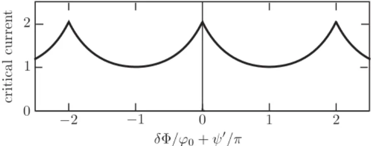
In the high-temperature regime the critical current is δ independent, while at low temperatures it varies by a factor of 2 on variation ofδ(see Fig.4). The oscillations of the critical current as a function of the flux through the normal region are reminiscent of the Fraunhofer oscillations in a conventional Josephson junction,24 but the minima are not at zero and
the periodicity is 2ϕ0 rather thanϕ0. These are characteristic signatures of a supercurrent carried by edge states rather than bulk states.25,26
The low-temperature supercurrent decays ∝1/L3 if the separationLof the NS interfaces is increased at constant width W. This is the characteristic decay of the spin-triplet proximity effect in a single transport channel.22
C. Meissner phase
In the Meissner phaselm> λwe may take ans-independent vector potential AAR along each NS interface, given by Eq. (2.10). If we also takes-independent parametersvc and
FIG. 4. Low-temperature critical currentIc as a function of the fluxδthrough the normal region, plotted from Eq. (4.11) in units ofe|12|/τ03.
v, the two quantities n andαn defined in Eqs. (4.6) and (4.7) are given by
n=τeiαn sinαn
αn
, αn=π W AAR/ϕ0, (4.14)
with τ=W v/v2c. (We kept the subscript n to allow for possibly different values ofAARat the two NS interfaces.)
The zero-temperature limit (4.11) of the supercurrent then takes the form
I()= e π
τ2
τ03 sin(2π /ϕ0)F(π δ/ϕ0+α1+α2)
×sinα1sinα2 α1α2
, (4.15)
with the functionFdefined in Eq. (4.13).
The phase shift in thedependence has disappeared, so now the supercurrent is an odd function of the fluxthrough the ring, vanishing at=0. SincedI /d >0 at=0 (for α1=α2), the supercurrent isparamagnetic, in contrast with the usual diamagnetic Josephson effect. Such a π junction appears generically in the spin-triplet proximity effect.22The main effect of the phaseαnaccumulated by the vector potential along the NS interface is the reduction of the critical current by the factor (sinα1sinα2)/(α1α2); the supercurrent vanishes ifα1orα2is a (nonzero) integer multiple ofπ.
From Eq. (4.15) we conclude that the scaling of the critical current with the parameters of the Josephson junction is given in the Meissner phase by
Ic eτ2
τ03
l2 m
W2 eωc(d/ lso) 2
(lm/L)3, (4.16)
withL=2(L+W) the length of the perimeter of the normal region. (All coefficients of order unity are disregarded in this scaling estimate, as well as any oscillatory dependence onW.)
D. Mixed phase
reaches its maximal value Icmax at δ= −(α1+α2)ϕ0/π, given according to Eq. (4.11) by
Icmax=2π e
3τ03|12|. (4.17)
The 1/L3 scaling with the separation of the NS interfaces is unchanged, but the scaling with the width W depends on the statistics ofAn(s), which determines the statistics ofn according to Eq. (4.6).
We have calculated the average of Imax
c for a random variation of An(s) as a function of s, with zero average and correlation length of orderlm (the average separation of vortices). The magnitude of the fluctuations is quantified by taking a piecewise constantAn(s) in each segment of length lm, drawn from a Gaussian distribution with zero average and standard deviationσ×ϕ0/π lmwithσof order unity. We have found that the average critical current in the mixed phase scales forW lmas
Icmaxeτ 2 τ3
0 lm W eωc
d2 l2
so l2
mW
L3 , (4.18)
larger than in the Meissner phase by a factorW/ lm.
V. COMPARISON WITH SPIN-SINGLET SUPERCURRENT A. Transfer matrix
It is instructive to compare the results of the previous section for the spin-triplet supercurrent with the spin-singlet case considered by Ma and Zyuzin.7,8For that purpose we assume spin degeneracy in the 2D electron gas, neglecting Zeeman splitting or spin-orbit coupling. Electron-hole symmetry now relates excitations from opposite spin bands, say an electron from the spin-up band and a hole from the spin-down band (or vice versa).
The effective Hamiltonian of a spin-singlet edge channel, to linear order in momentum, is
H =
1
2{vc,p−eA} ∗ 12{vc,p+eA}
, (5.1)
fully constrained by Hermiticity and the electron-hole sym-metry requirement
σyH∗σy = −H. (5.2)
Choosing a gauge so thatis real we now have
H =vc(p−eAσz)+σx−12ivc. (5.3)
The key difference with the effective Hamiltonian (2.5) for a spin-triplet edge channel is that the coupling between electrons and holes does not vanish atp=0 in the spin-singlet case.
We now follow the same steps as in Sec.II E. The particle current operator
J =∂H /∂p=vc (5.4)
transformsHto
˜
H =J−1/2H J−1/2=p−eAσz+(/vc)σx (5.5)
and produces the unitary transfer matrix
M(s2,s1)=Psexp
i
s2
s1 ds
ε−σx vc
+eAσz . (5.6)
The transfer matrix no longer commutes with σz at ε=0, so there is no low-energy suppression of Andreev reflection as in the spin-triplet case. The order parameter equals 0 along the NS interface and zero along the normal boundary.
B. Meissner phase
We consider the Meissner phase lm> λ, with an s -independent vector potentialAnalong the interface with Sn. Taking also ans-independentvc, we can evaluate Eq. (5.6) without the complications from operator ordering. The scat-tering matrix becomes
S(ε)=eiετ0ei(π/ϕ0)(+δ/2)σzM˜
2 ×e−i(π/ϕ0)(−δ/2)σzM˜
1, (5.7)
˜
Mn= exp[ieW Anσz−i(0W/vc)σx], (5.8)
withτ0=2(L+W)/vc. The supercurrent follows from
I()= d d
∞
p=0
2kBT ln det [1−S(iωp)], (5.9)
which differs from Eq. (3.4) by a factor of 2 because of spin degeneracy of the edge channel in the spin-singlet case.
Substitution of Eq. (5.7) into Eq. (5.9) gives
I()= −4π kBT
ϕ0 sin(2π /ϕ0)(W/ξc) 2sin2β
β2
×
∞
p=0
[cosh(ωpτ0)+X]−1, (5.10)
X =[cos(2π /ϕ0)−cos(π δ/ϕ0)](W/ξc)2sin 2β
β2
+(π W AAR/ϕ0) sin 2β
β sin(π δ/ϕ0)
−cos 2βcos(π δ/ϕ0), (5.11)
β =(π W AAR/ϕ0)2+(W/ξc)2. (5.12)
(For a compact expression, we took A1 =A2≡AAR.) We defined the length ξc=hv¯ c/0, which is smaller than the superconducting coherence lengthξ0=hv¯ F,S/0by a factor vc/vF,S. In the point contact limitW→0 considered by Ma and Zyuzin our result (5.10) agrees with their finding (Eq. 13 of Ref.8).
At zero temperature Eq. (5.10) is
I()= − 4e π τ0
sin(2π /ϕ0)(W/ξc)2sin 2β
β2
×√ 1
1−X2 arctan
1−X √
1−X2
In contrast to the spin-singlet result (4.11), the dependence of the supercurrent on the fluxthrough the ring is strongly nonsinusoidal. The critical current oscillates both as a function of the fluxδthrough the normal region and as a function of the widthWof the NS interface. At high temperature only the oscillation withW remains,
I()= −8ekBTsin(2π /ϕ0)(W/ξc)2 sin2β
β2 e
−π kBT τ0,
(5.14)
while thedependence is now sinusoidal.
On increasing the separation L of the NS interfaces the spin-singlet supercurrent (5.13) in the low-temperature limit decays as 1/L. This is in contrast to the 1/L3 decay of the spin-triplet supercurrent (4.11). In the high-temperature limit, the supercurrent has the same exponential decay ∝ exp(−π kBT τ0) in the spin-singlet and spin-triplet cases and only the pre-exponentials differ [cf. Eqs. (4.10) and (5.14)].
The spin-singlet supercurrent in the high-temperature regime has been studied also by Ishikawa and Fukuyama,27
without taking the point contact limit W →0 of Refs. 7
and8. We have not been able to reconcile their result with our Eq. (5.14), because only the length L of the normal boundaries enters into their exponential decay (rather than the sumL+Wof the lengths of normal and superconducting boundaries). The very recent study by Stone and Lin,18which
also includes finite-W effects, still assumesW Lso it does not distinguish between the two decay rates.
C. Narrow-contact regime
The full expression (5.13) for the zero-temperature spin-singlet supercurrent simplifies considerably in the
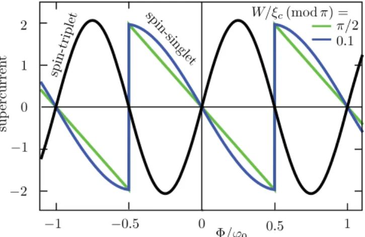
narrow-FIG. 5. (Color online) Zero-temperature supercurrent as a func-tion of the fluxthrough the ring, for a fluxδthrough the normal region equal to an integer multiple of 2ϕ0=h/e. The green and blue
curves (in units of (e/τ0)|sinW/ξc|) are the spin-singlet result (5.13) for two values ofW(in the narrow-contact regimeWlm, so with
AAR→0). The black curve is the spin-triplet result (4.11) plotted
in units of eτ2
/τ
3
0. For the sake of comparison we also took the
narrow-contact limit of the spin-triplet result, settingα1,α2→0 in
Eq. (4.11).
FIG. 6. (Color online) Low-temperature critical current as a function of the flux δ through the normal region. The dashed curve is the spin-triplet result (4.11), plotted in units ofeτ2
/τ
3 0 (in
the narrow-contact limitα1,α2→0). The solid curves (in units of
(e/τ0)|sinW/ξc|) follow from the spin-singlet result (5.13) for three values ofWin the narrow-contact regime. The resonance at integer
δ/2ϕ0 peaks atIc=(2π/3)eτ2/τ
3
0 in the spin-triplet case and at
Ic=(2e/τ0)|sinW/ξc|in the spin-singlet case.
contact regimeW lm, when we may setAAR→0. (This is the regime considered by Stone and Lin.18) Note that
ξc/ lmhω¯ c/01, soW may still be large compared to ξc in the narrow-contact regime. As shown in Fig. 5, the current-phase relationship in the narrow-contact regime has a sawtoothlike shape, consistent with Ref.18.
For reduced widthw≡W/ξc(moduloπ) much less than unity the critical current exhibits resonant peaks (of height 2ew/τ0) whenever δ/2ϕ0 is an integer. (See Fig. 6, blue and red curves.) Forw→π/2 the critical currentIc=2e/τ0 becomesδ-independent (green line in Fig.6), signifying the absence of Fraunhofer oscillations.
VI. CONCLUSION
In conclusion, we have analyzed the Josephson effect in the lowest Landau level, both with and without spin polarization. The critical current scales differently with the parameters of the Josephson junction in these two cases. Without spin polarization we have the spin-singlet Josephson effect considered earlier,7,8,18with low-temperature scaling
Ic,singleteωc lm
L, (6.1)
inversely proportional to the lengthLof the perimeter of the normal region.
We have found that a spin-polarized Landau level can still carry a supercurrent. The low-temperature scaling of this spin-triplet Josephson effect is
Ic,tripleteωc
lm
L 3
(W/ lm)(d/ lso)2, (6.2)
ForW Lthe ratio of spin-triplet and spin-singlet critical currents is of order
Ic,triplet/Ic,singlet(lm/L)(d/ lso)2. (6.3)
The spin-orbit scattering length in InAs is of order lso 100 nm, which could well be of the same order as the electrostatic lengthd (the smoothness of the potential step at the NS interface). The main reason for the relative smallness of the spin-triplet supercurrent is then the factorlm/L. Since lm25 nm forB 1 T, a submicron junction is needed for an observable effect. (The 1 T magnetic field scale is well below the upper critical field of 14 T of a NbN superconductor.) As we have shown, the spin-triplet Josephson effect has unusual features, including a paramagnetic, rather than diamagnetic, current-phase relationship, and Fraunhofer oscillations which have ah/erather thanh/2eperiodicity.
For the purpose of comparison with the spin-singlet Joseph-son effect, we have performed an analysis that goes beyond earlier work on that problem,7,8,18 in particular with regard
to the Fraunhofer oscillations. We have found a remarkable dependence of the amplitude of the Fraunhofer oscillations on the relative magnitude of the junction widthWand an effective coherence lengthξc. ForW/ξc=π/2 (modπ) the Fraunhofer oscillations vanish altogether (see Fig.6).
These spin-singlet results may well be of relevance also for graphene, which is an attractive alternative to InAs in the search for the coexistence of the Josephson and quantum Hall effects. The results obtained here would apply ifW is larger than the intervalley scattering length. For smallerWthe valley selectivity of the edge states enters, along the lines described in Ref.31.
ACKNOWLEDGMENTS
This research was supported by the Dutch Science Foun-dation NWO/FOM, by the Eurocores program EuroGraphene, and by an ERC Advanced Investigator grant.
APPENDIX: ANDREEV-RASHBA EDGE STATES The theory of Andreev edge states, produced by the interplay of cyclotron motion and Andreev reflection, has been developed by Z¨ulicke and collaborators.4,20,28 Here we
include the interplay with Rashba spin-orbit interaction in the spin-polarized regime where Andreev reflection can only occur because of the Rashba effect.
The theory is complicated by the fact that we are deep in the quantum mechanical regime, with only one occupied Landau level, and cannot make the semiclassical approximation of large Landau level index made in earlier work.4,20,28,29Since the Fermi energy in the normal metal is small compared to the superconducting gap, we can also not make the usual Andreev approximation (matching wave amplitudes without matching derivatives). We keep the theory tractable analytically by treating the spin-orbit interaction perturbatively.
The goal of our analysis of the Andreev-Rashba edge states is to arrive at a microscopic derivation of the parameters that enter into the effective edge-state Hamiltonian (2.3), on which our theory of the spin-triplet Josephson effect is based.
1. Bogoliubov-De Gennes equation
We start from the Bogoliubov-De Gennes (BdG) equation
H0−EF τy
∗τy EF−H0∗
ψe ψh
=ε
ψe ψh
, (A1)
for quasiparticle excitations consisting of an electron spinor ψe=(u+,u−) and a hole spinor ψh=(v+,v−). The label ± indicates the spin band and the Pauli matrix τy acts on the spin degree of freedom. The pair potentialof a spin-singlet superconductor couples electron and hole excitations in opposite spin bands. Electron-hole symmetry is expressed byσxH∗σx= −H.
The single-particle Hamiltonian
H0=(2m)−1(p−eA)2+V +1
2gμBB·τ+HR, (A2)
HR=α(py−eAy)τx−α(px−eAx)τy, (A3)
contains the kinetic energy, potential energy, Zeeman energy, and Rashba spin-orbit interaction. We consider a translation-ally invariant NS interface aty=0, with vector potentialA= A(y) ˆx, magnetic field B= −A(y)ˆz, electrostatic potential V =V(y), and pair potential=(y). The effective mass m, effective gyromagnetic factorg, and Rashba coefficientα are taken spatially uniform (otherwise also derivatives ofm andα would have to enter in the Hamiltonian, to preserve Hermiticity).
Parallel momentumpx ≡pis conserved for states∝eipx. Theydependence of the wave functions is determined by
H0= − 1 2m
d2 dy2 +
[p−eA(y)]2
2m +V(y)
−1 2gμBA
(y)τ
z+HR, (A4)
HR = −iατx d
dy −α[p−eA(y)]τy. (A5)
In this basis the operators H0,H0∗ in the BdG Hamiltonian should be replaced byH0(p),H0∗(−p).
The NS interface is aty=0, with the superconductor in the regiony <0. In the simplest model for the interface we take a step function both for the pair potential,(y)=0θ(−y), and for the electrostatic potential, V(y)= −V0θ(−y) with V0>0. [The function θ(y) equals 1 for y >0 and 0 for y <0.] Smoothing of the interface is important and will be considered at the end of the Appendix. We assume that we are deep in the Meissner phase,lm λ, so we may neglect the penetration of the magnetic field in the superconductor. In the gauge where0is real, the vector potential is then given simply byA(y)= −yBθ(y).
2. Solution without the Rashba effect a. Eigenstates in S
In S (fory <0) the BdG Hamiltonian withHR =0 is given by
HS=
⎛ ⎜ ⎜ ⎜ ⎜ ⎝
μ(p)−κ∂2
y 0 0 −i0
0 μ(p)−κ∂2
y i0 0
0 −i0 −μ(p)+κ∂2
y 0
i0 0 0 −μ(p)+κ∂2
y
⎞ ⎟ ⎟ ⎟ ⎟
⎠, (A6)
withμ(p)=p2/2m−V
0−EF,κ=(2m)−1, and∂y =d/dy. There are four eigenstatesχs,±w±(y) ofHSfor 0< ε < 0 (decaying fory→ −∞), with
w±(y)=eiq±y, γ
±=ε±i
2
0−ε2, (A7)
κq±2 = −μ(p)±i
20−ε2, Imq
±<0, (A8)
χ↑,± =
⎛ ⎜ ⎝
γ± 0 0 i0
⎞ ⎟
⎠, χ↓,±=
⎛ ⎜ ⎝
0 i0
γ∓ 0
⎞ ⎟
⎠. (A9)
For 0 EF+V0 ≡EF,S≡pF,S2 /2m we may approxi-mate
q±= ∓q(p)− im q(p)
2
0−ε2, q(p)=
p2
F,S−p2.
(A10)
b. Eigenstates in N
In N (fory >0) we have, again forHR =0,
HN =
⎛ ⎜ ⎜ ⎜ ⎜ ⎝
U(p,y)−κ∂2
y+μ+ 0 0 0
0 U(p,y)−κ∂2
y +μ− 0 0
0 0 −U(−p,y)+κ∂2
y −μ+ 0
0 0 0 −U(−p,y)+κ∂y2−μ−
⎞ ⎟ ⎟ ⎟ ⎟
⎠, (A11)
withμ±= ±12gμBB−EF andU(p,y)=(p+eBy)2/2m. The differential equation
U(p,y)−κ∂y2+μ±φ(y)=εφ(y), (A12)
withφ(y)→0 fory→ ∞is solved by a parabolic cylinder functionU,
φ±(ε,p,y)=Cε,p± U
μ±−ε ωc
,√2
y lm
+plm . (A13)
The normalization constantCε,p± =O(l−m1/2) is determined by
∞
0
φ±2(ε,p,y)dy =1. (A14)
The parabolic cylinder function U(−ν,y) has no nodes as a function ofy forν1/2 and only a single node for 1/2< ν3/2.
The four eigenstates ofHN are constructed in terms of the functionsφ±,
ψe↑=
⎡ ⎢ ⎣
φ+(ε,p,y) 0 0 0
⎤ ⎥
⎦, ψe↓=
⎡ ⎢ ⎣
0 φ−(ε,p,y)
0 0
⎤ ⎥ ⎦,
ψh↑=
⎡ ⎢ ⎣
0 0 φ+(−ε,−p,y)
0
⎤ ⎥
⎦, ψh↓ =
⎡ ⎢ ⎣
0 0 0 φ−(−ε,−p,y)
⎤ ⎥ ⎦.
(A15)
c. Matching at the NS interface
We construct two independent superpositions of basis states in N and S,
1(y)=θ(y)[a1ψh,↑(y)+b1ψe,↓(y)]
+θ(−y)[c1χ↓,+eiq+y+d1χ↓,−eiq−y], (A16a)
2(y)=θ(y)[a2ψe,↑(y)+b2ψh,↓(y)]
We chooseεsuch that
(ε−μ+)/¯hωc< 1
2 <(ε−μ−)/hω¯ c< 3
2. (A17) In this range the equationφ+(ε,p,0)=0 has no solution while the equationφ−(ε,p,0)=0 has a single solutionp=D(ε). As we will see, this is the branch of the dispersion relation with wave function1, while another branch, with wave function 2, is given byp= −D(−ε).
Continuity of1andd1/dyaty =0 gives four equations for the coefficientsa1,b1,c1,d1,
a1φ+(−ε,−p,0)=c1γ−+d1γ+, (18a)
b1φ−(ε,p,0)=i0(c1+d1), (18b)
a1φ+(−ε,−p,0)=iq+c1γ−+iq−d1γ+, (18c)
b1φ−(ε,p,0)= −0(q+c1+q−d1), (18d)
withφ± =dφ±/dy. The solution satisfies
c1 d1
= −γ+ γ−
q−φ+(−ε,−p,0)+iφ+(−ε,−p,0)
q+φ+(−ε,−p,0)+iφ+(−ε,−p,0)
= −γ+q−
γ−q+[1+O(λF,S/ lm)], (A19)
sinceφ+ is smaller thanq±φ+by a factorλF,S/ lm1 (with λF,S=2π/kF,S). [Here we have used thatφ+does not vanish forεin the range (A17).]
Similarly, for2we have the matching conditions
a2φ+(ε,p,0)=c2γ++d2γ−, (A20a)
b2φ−(−ε,−p,0)=i0(c2+d2), (A20b)
a2φ+(ε,p,0)=iq+c2γ++iq−d2γ−, (A20c)
b2φ−(−ε,−p,0)= −0(q+c2+q−d2), (A20d)
with the solution
c2 d2 = −
γ− γ+
q−φ+(ε,p,0)+iφ+(ε,p,0) q+φ+(ε,p,0)+iφ+(ε,p,0)
= −γ−q−
γ+q+[1+O(λF,S/ lm)]. (A21)
The normalization requirement gives one more equation for each set of coefficients,
|an|2+ |bn|2+ q(p) 2 0
m
2 0−ε2
(|cn|2+ |dn|2)=1. (A22)
d. Dispersion relation
Since
γ+q−
γ−q+ =1+O(ε/0)+O(λF,S/ξ0), (A23)
we may approximate c1
d1 = −1= c2
d2 for ε0 and λF,Sξ0,lm. (A24)
Equations (18b) and (A20b) then give the dispersion relations
ε1(p)=Dinv(p)≡εp, for 1, (A25a)
ε2(p)= −Dinv(−p)≡ −ε−p, for 2, (A25b)
withεpdetermined by the equation
φ−(εp,p,0)=0⇒U
μ−−εp
ωc
,√2plm =0. (A26)
The dispersion relation of the two modes is plotted in Fig.2. For smallpit is approximately linear, given by
εp=vc(p−eAAR), (A27)
with the definitions
vc=1.14lmωc, evcAAR=
ν−−32ωc, ⇒AAR=0.88
ν−−32lmB≡ −cmlmB, (A28)
ν−= EF + 1 2gμBB ¯ hωc
. (A29)
These results provide the numerical coefficients forvcandAAR in Eqs. (2.8) and (2.10).
Concerning the coefficientcm, we note that, as required by Eq. (A17), the value ofν− at the Fermi level is in the range 1/2< ν−<3/2. The ratiogμBB/¯hωc=gm/2m0 (withm0 the free electron mass) is typically much smaller than unity, soν− ≈1/2 will be close to the lower end of this range and cm≈0.88.
e. Eigenstates
From the matching conditions we determine the coefficients of the zeroth-order eigenstates,
a1
d1
= 2i0
φ+(−εp,−p,0) ≡Y1,
a2
d2
= −2i0 φ+(−ε−p,p,0)
≡Y2,
(A30a) b1
d1 =
−20q(p) φ−(εp,p,0) ≡
X1, b2 d2 =
20q(p) φ−(ε−p,−p,0) ≡
X2.
(A30b)
It follows that
an/bn=O(λF,S/ lm)1. (A31)
This means that1and2in the normal region have most of their weight in the spin-down band, so1is predominantly an electron state and2is predominantly a hole state.
The normalization condition (A22) simplifies to
|bn|2+Y0|dn|2=1, Y0≡2q(p)0/m. (A32) Together with Eq. (A30) this determines all coefficients (up to an overall phase factor),
an=Yn
Xn2+Y0
−1/2
, bn=Xn
Xn2+Y0
−1/2 ,
dn= −cn=
X2n+Y0
−1/2
. (A33)
Becauseφ−(εp,p,0)=O(lm−3/2), we can estimate
Y0 X2 n
=O
ξ0λ2F,S
l3 m
since we work in the regime wherelmis large both compared to λF,Sand compared toξ0. We may therefore neglectY0relative toX2
n.
3. Inclusion of the Rashba effect We include the Rashba Hamiltonian
δH =
HR 0 0 −HR∗
(A35)
as a perturbation of the BdG Hamiltonian. To lowest or-der in this perturbation we need the matrix elements of δH in the basis of unperturbed eigenstates 1,2. Since n|δH |n =0, there is only a single matrix element 2|δH|1 = 1|δH |2∗ to consider. We calculate separately the contributions to this matrix element from the superconducting and normal regions.
a. Matrix element in S
The Rashba Hamiltonian in the superconducting region is
δHS=
−iατx∂y−αpτy 0
0 −iατx∂y+αpτy
. (A36)
Note that
χ↑,±|δHS|χ↓,±S=0, (A37) where · · ·S indicates integration over the superconducting regiony <0. The matrix element becomes
2|δHS |1S=iα0
20−ε2[c∗
2d1(1+ip/q−) −c1d2∗(1+ip/q+)]. (A38)
With the help of the approximation
c∗2d1 c1d2∗
≈(γ−/γ+)2, (A39)
this gives, forε0,
2|δHS|1S=α20c1d2∗(p/q+−p/q−). (A40)
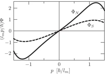
FIG. 7. Plot of the functionspS(p) andpN(p), which de-termine the contribution to the Rashba matrix elements (A41) and (A47) from the superconducting and normal region, respectively. The curves are calculated from Eqs. (A42) and (??), for Fermi energyEF= 12¯hωc. These two functions are of the same order of magnitude, but the contribution to the Rashba matrix element from S has an additional prefactor (kF,Slm)−2, so it is much smaller than the contribution from N.
Sinceq±= ∓pF,S[1+O(λF,S/ξ0)+O(p/pF)2], we may further approximate
2|δHS|1S= −2α20c1d2∗ p pF,S
= 2α20p pF,S|X1X2|
= αp
(kF,Slm)3
S(p), (A41)
where we have used Eqs. (A33) and (A34), and we have introduced a dimensionless even function ofp,
S(p)=12lm|3 φ
−(ε−p,−p,0)φ−(εp,p,0)|. (A42) See Fig.7 for a plot ofpS(p), which is an approximately linear function ofp, given for smallpby
lmpS(p)=1.13lmp+O(lmp)2. (A43)
b. Matrix element in N
The Rashba Hamiltonian in the normal region is
δHN =
−iατx∂y−α(eBy+p)τy 0
0 −iατx∂y−α(eBy−p)τy . (A44)
The matrix element is
2|δHN|1N =iαa2∗b1φ+(−ε−p,p,y)| −∂y+eBy+p|φ−(εp,p,y)N
with the coefficients given by Eq. (A33),
a2∗b1= − Y2X1 |X1X2|, b
∗
2a1 = X2Y1
|X1X2|. (A46) The matrix element can be written in the form
2|δHN |1N = αp kF,Slm
N(p), (A47)
in terms of a dimensionless even function ofp,
N(p)=(p)+(−p), (A48a)
(p)= 1 p
|φ−(ε−p,−p,0)φ−(εp,p,0)| φ−(εp,p,0)φ+(−ε−p,p,0)
φ+(−ε−p,p,y)|
× y lm
+plm−lm∂y |φ−(εp,p,y)N. (A48b)
In Fig.7we have also plottedpN(p). Thepdependence is approximately linear, given for smallpby
lmpN(p)=cNlmp+O(lmp)2. (A49)
The coefficient cN is a function ofEF/hω¯ c, of order unity. ForEF = 12hω¯ c(Fermi level half-way between the splin-split lowest Landau level) one hascN =1.98.
4. Andreev-Rashba edge states at an abrupt NS interface From Eqs. (A41) and (A47) we find that the matrix element of the Rashba Hamiltonian in the unperturbed basis is
2|δH |1 = αp kF,Slm
[N(p)+(kF,Slm)−2S(p)].
(A50)
Since both functions N(p) and S(p) are of order unity for p of order 1/ lm, the effect of spin-orbit coupling in the superconductor on the Andreev-Rashba edge states is weaker by a factor 1/(kF,Slm)2 ¯hωc/EF,S than the effect of spin-orbit coupling in the normal region. We therefore arrive at the final result for the Rashba matrix element,
2|δH|1 = αp kF,Slm
N(p). (A51)
To first order in the Rashba coefficient α, the BdG Hamiltonian in the unperturbed basis is a 2×2 matrix H with elements
H=
εp (αp/kF,Slm)N(p) (αp/kF,Slm)N(p) −ε−p
. (A52)
The matrix elements have an approximately linearp depen-dence,
H≈
vc(p−eAAR) vp vp vc(p+eAAR)
, (A53)
with coefficients vc and AAR given by Eq. (A28). The coefficientvfollows from Eq. (A49),
v=cN α kF,Slm
vc kF,Slso
, (A54)
in terms of the spin-orbit scattering lengthlso =¯h2/mα. The dispersion relation of the Andreev-Rashba edge states, to second order in the Rashba coefficientα, is given by
ε±=vcp±
(evcAAR)2+(vp)2, (A55)
with the+sign for the electron-like mode1and the−sign for the holelike mode2.
5. Andreev-Rashba edge states at a smooth NS interface So far we have taken an abrupt model for the NS interface, with a step function both in the pair potential (from 0 to0) and in the electrostatic potential (from 0 to−V0). We now turn to the more realistic model of a smooth interface. Since0 EF,Swe do not expect the abruptness of the pair potential step to have significant consequences, so we keep the step function (y)=0θ(−y).
The situation differs for the electrostatic potential step, which enforces normal reflections at the expense of Andreev reflections. We therefore broaden the step in V(y) over a distanced, such thatV(y)= −V0fory−d andV(y)=0 for y0. The abrupt limit corresponds tod 1/kF,S. We now takedlarger, but still small compared toξ0.
a. Eigenstates in S
The eigenstates in N are unaffected by the smoothing for y <0. The eigenstates in S are given byχs,±w±(y), with the same spinor χs,± defined in Eq. (A9) and a spatial profile w±(y) determined by
−∂y2w±(y)=2m[−μ(p,y)±i
20−ε2]w
±(y), (A56)
μ(p,y)=p2/2m+V(y)−EF. (A57)
Since we assume d ξ0 we may solve the scatter-ing by the potential step independently of the reflection from the pair potential. The wave vector (in the limit ε→0) changes from k(p)=2mEF −p2 at y =0 to k(p)=2m(EF+V0)−p2 at y= −d. Plane-wave solu-tions a+eiky+a−e−iky at y =0 are related to plane-wave solutionsa+eiky+a
−e−ikyaty= −dby a unitary scattering
matrix,
a+ a−
=
r t t r
a− a+
. (A58)
The solutionw±(y) corresponds to settinga∓=0. We thus obtain
w+(0)
iw+(0) =k(p) r−1 r+1,
w−(0)
iw−(0) = −k(p) r∗−1
r∗+1, (A59)
withw± =dw±/dy. The complex conjugation appears as a result of inversion of the scattering matrix, but it can be ignored because the reflection amplituderis real forkd1.
b. Matching at the NS interface
Matching of the eigenstates in N to those in S aty =0 proceeds entirely as in the case of the abrupt interface, with q±replaced by the logarithmic derivativew±(0)/ iw±(0). The result (A30) for the matching coefficients changes simply by the replacement ofq(p) by
qeff(p)= w
−(0)
iw−(0) =k(p) 1−r
The Fermi wave vectorkF,S=q(0) is replaced by
keff =qeff(0)=k(0)1−r
1+r. (A61)
The reflection amplituder is related byr = −√1−T to the overbarrier transmission probabilityT. Sinced ξ0and k1/ lm1/ξ0, we necessarily havekdd/ lm1. One may then expand
T =cbarrierkd+O(kd)2, (A62) withcbarrier a numerical coefficient of order unity. The wave vectorkefftakes the form
keff = 4k(0)
T =
4 cbarrierd
. (A63)
The value ofcbarrierdepends on the shape of the barrier. As an example, we take the Woods-Saxon step
V(y)= −V0[1+e(y+y0)/d]−1, (A64)
withy0d (so the potential is essentially zero fory >0). The transmission probability is30
T =1−sinh
2[π d(k−k)]
sinh2[π d(k+k)]
=4π kdcotanh (π kd)+O(kd)2. (A65) For a step that is smooth on the scale of λF,S (so kd d/λF,S1) we arrive at Eq. (A62) withcbarrier=4π, hence
keff=1/π d. In the opposite regime kd →0 of an abrupt potential step we haveT =4k/k, hence keff =k(0), as it should be.
c. Dispersion relation
The zeroth-order dispersion relation, which is independent of q(p), remains unchanged, still given by Eqs. (A25) and (A26), and also the velocityvcremains given by Eq. (A28).
The expression (A51) for the Rashba matrix element in the unperturbed basis is changed into
2|δH|1 = αp kefflm
N(p), (A66)
with the same function N as for the abrupt interface (see Fig. 7). Once again, the dominant contribution to the matrix element comes from the normal region, with the contribution from the superconducting region smaller by a factor (kefflm)−2(d/ lm)2.
The BdG Hamiltonian in the unperturbed basis still has the form (A53), with the only difference appearing in the coefficientv. Instead of Eq. (A54) for the abrupt interface it is now given by
v=cN α kefflm
vcd
lso . (A67)
This is the result (2.8) used in the analysis of the spin-triplet Josephson effect.
1B. I. Halperin,Phys. Rev. B25, 2185 (1982). 2A. F. Andreev, Sov. Phys. JETP19, 1228 (1964). 3Y. Takagaki,Phys. Rev. B57, 4009 (1998).
4H. Hoppe, U. Z¨ulicke, and G. Sch¨on,Phys. Rev. Lett.84, 1804
(2000).
5Y. Asano,Phys. Rev. B61, 1732 (2000). 6N. M. Chtchelkatchev,JETP Lett.73, 94 (2001).
7M. Ma and A. Yu. Zyuzin,Europhys. Lett.21, 941 (1993). 8A. Yu. Zyuzin,Phys. Rev. B50, 323 (1994).
9M. P. A. Fisher,Phys. Rev. B49, 14550 (1994).
10T. D. Moore and D. A. Williams,Phys. Rev. B59, 7308 (1999). 11F. S. Bergeret, A. F. Volkov, and K. B. Efetov,Phys. Rev. Lett.86,
4096 (2001); Rev. Mod. Phys.77, 1321 (2005).
12A. Kadigrobov, R. Shekhter, and M. Jonson,Europhys. Lett.54,
394 (2001).
13M. Eschrig,Phys. Today64, 43 (2011).
14M. G. Pala, M. Governale, U. Z¨ulicke, and G. Iannaccone,Phys.
Rev. B71, 115306 (2005).
15H. Takayanagi and T. Akazaki,Physica B249-251, 462 (1998). 16J. Eroms, D. Weiss, J. De Boeck, G. Borghs, and U. Z¨ulicke,Phys.
Rev. Lett.95, 107001 (2005).
17I. E. Batov, Th. Sch¨apers, N. M. Chtchelkatchev, H. Hardtdegen,
and A. V. Ustinov,Phys. Rev. B76, 115313 (2007).
18M. Stone and Y. Lin, e-printarXiv:1102.5265v2.
19H. B. Heersche, P. Jarillo-Herrero, J. B. Oostinga, L. M. K.
Vandersypen, and A. F. Morpurgo,Nature446, 56 (2007).
20F. Giazotto, M. Governale, U. Z¨ulicke, and F. Beltram,Phys. Rev.
B72, 054518 (2005).
21F. Rohlfing, G. Tkachov, F. Otto, K. Richter, D. Weiss, G. Borghs,
and C. Strunk,Phys. Rev. B80, 220507(R) (2009).
22B. B´eri, J. N. Kupferschmidt, C. W. J. Beenakker, and P. W.
Brouwer,Phys. Rev. B79, 024517 (2009).
23P. W. Brouwer and C. W. J. Beenakker,Chaos Solitions Fractals8,
1249 (1997).
24M. Tinkham, Introduction to Superconductivity (McGraw-Hill,
New York, 1996).
25J. P. Heida, B. J. van Wees, T. M. Klapwijk, and G. Borghs,Phys.
Rev. B57, R5618 (1998).
26V. Barzykin and A. M. Zagoskin,Superlattices Microstruct.25, 797
(1999).
27Y. Ishikawa and H. Fukuyama, J. Phys. Soc. Jpn. 68, 954
(1999).
28U. Z¨ulicke, H. Hoppe, and G. Sch¨on,Physica B298, 453 (2001). 29P. Rakyta, A. Korm´anyos, Z. Kaufmann, and J. Cserti,Phys. Rev.
B76, 0645162007.
30Z. Ahmed,J. Phys. A32, 2767 (1999).
31A. R. Akhmerov and C. W. J. Beenakker, Phys. Rev. Lett.98,