Examining Causal Chains Between Real US GDP and Energy Consumption Through Mixed Frequency Granger Causality Testing
By: Clayton Hackney
Honors Thesis Economics Department
The University of North Carolina at Chapel Hill
April 2015
Approved:
Abstract
This paper explores potential short-term causal relationships between energy consumption and real GDP in the United States from 1982-2006. Despite extensive study, there is no agreed upon consensus about the existence and nature of such a relationship. A primary issue in the literature is that existing studies are plagued by temporal aggregation issues due to inconsistency of data sampling (quarterly GDP and monthly energy consumption samples). We address this issue by conducting a Granger Test for Causality on rolling windows with parametrically bootstrapped residuals per Goncalves and Kilian (2004) in a bivariate Mixed Frequency Vector
Acknowledgements
1. Introduction
The existence and direction of causality between energy consumption and real U.S. GDP has been widely debated since the oil shocks of the 1970s (Kraft and Kraft, 1978). The question in particular is whether or not energy conservation policy will negatively impact income, and the convention of the 2005 Kyoto Protocol brought the issue back into focus. (Salamaki and Venetis, 2013). 1
If uni-directional causality is determined to run from energy consumption to income, then this would indicate an economy that is dependent upon energy, and concerns about the negative income effects of energy conservation would be supported (Masih and Masih, 1998).
Uni-directional causality from income to energy consumption is indicative of an economy less dependent upon energy consumption, and energy conservation policy would be expected to have less of an impact upon income (Jumbe, 2004). Should no causal link be determined, energy conservation policy would not be expected to have any impact on income, called the “neutrality hypothesis” (Yu and Choi, 1985).
It seems intuitive there should be some short-term causal relationship between real GDP and energy consumption, and this relationship might take many forms. For instance, fluctuations in energy prices in one period might affect the amount a firm would want to produce in the next period due to price expectations and budget constraints. The resulting net effect upon economic growth is ambiguous since there would be an interplay between firms that are negatively affected
1 In 1997 the U.S. Senate passed the Byrd-Hagel Resolution, which expressed disapproval of any international
by higher input prices and firms that benefit from higher energy prices. Economic growth might impact energy consumption through increased investment in capital which demand more energy consumption to operate or maintain. For growth models that incorporate technology innovations, new advancements in technology that conserve energy or utilize different energy sources might impact energy consumption and real GDP simultaneously. Additionally, business cycles might impact both real GDP and energy consumption simultaneously, as short-term booms might incentivize upgrading to energy-conservative methods of capital at the same time as real GDP experiences growth. Thus, there are channels through which energy consumption might impact real GDP and vice-versa as well as outside influences that might impact the two simultaneously.
Most empirical studies have been based around bivariate Granger causality tests, and focus on country-specific bivariate vector autoregressions of energy consumption and real GDP. However, differences in econometric techniques and data selection have led to very different conclusions. As an example, in the seminal study by Kraft and Kraft (1978), uni-directional causality from GNP to energy consumption was found for the United States using data from 1947-1974. This study was later questioned by Akarca and Long (1980) who concluded the study was affected by “temporary sample instability” (Lee, 2006). Similarly, different findings have been found for the United States due to empirical method and period studied (Stern, 2000; Thoma, 2004; Soytas and Sari, 2003).
regression models to allow for series with different sampling frequencies to exist at their available frequencies.
This study seeks to apply a mixed frequency vector autoregression - developed by Ghysels (2012) - to a Granger Causality test of energy consumption and U.S. real GDP utilizing methodology developed by Ghysels, Hill, and Motegi (2014a,b) in order to address the effect of temporal aggregation on time series data. We use real growth in order to abstract from inflation over time and use a standard Wald test based on mixed frequency theory in Ghysels, Hill, and Motegi (2014b). We then perform causality tests over rolling windows of small subsamples across three models. One model is based on mixed frequency data where GDP is measured quarterly and energy is measured monthly. The two remaining models are based on using quarterly data, as the common low frequency with different methods of aggregating energy consumption data, a stock and flow method.
can be due entirely to the relationships between included and excluded variables, and not due to a true causal link between included variables.
This paper is organized as follows. Section 2 contains a literature review of past empirical techniques. Section 3 outlines our methodology and motivation. Data selection and modification are discussed in Section 4. In Section 5, we present our results and findings, and we conclude in Section 6. All tables and figures are collected after Section 6.
2. Literature Review
2.1 Theoretical Models
Causal links between energy and GDP have been discussed widely in the literature from various perspectives, and no single theoretical model has been agreed upon. All studies that include theoretical models attempt to demonstrate a channel through which energy affects GDP; however, none attempt to detail a channel through which GDP might determine energy. It appears as if they implicitly assume a positive relationship between GDP and energy, and this appears reasonable. Most neo-classical growth models decompose growth in terms of labor, capital and residual white noise, such as the Solow model. These models do not include energy in the production process, and thus energy consumption has no causal link with GDP, except through energy’s being subsumed by capital in the production process (since it is not labor).
external sources and labor in technological processes. In these models, energy-driven equipment replaces manual labor and functions as a production input (Pokrovski, 2003).
In order to conduct a test for causation,Salamaliki and Venetis (2013) model the causal relationship between energy consumption and economic growth on the “neo-classical one-sector aggregate production technology framework” as proposed by Ghali and El-Sakka (2004):
𝑌𝑡= 𝑓(𝐿𝑡, 𝐾𝑆𝑡, 𝐸𝐶𝑡)
where Y is real gross domestic product (GDP), KS is real capital stock, L is employment and EC is energy consumption. All variables are transformed into per capita form by dividing by labor in order to avoid collinearity between capital and labor as well as control for scale effects, as discussed in Lee et al. (2008) and Lee and Chien (2010). All variables are expressed in natural logarithms, and the per capita production function is of the form
𝐿𝑌𝑡 = 𝑓(𝐿𝐾𝑆𝑡, 𝐿𝐸𝐶𝑡)
where LYt = Yt / Lt , LKSt = KSt / Ltand LECt = Et / Lt .
2.2 Empirical Methods
2.2.1 Granger Causality Definition
In another literature, the debate is which methodology is best to evaluate and determine if there are causal links between energy and GDP. Most studies have focused on developing
testable hypothesis around so-called Granger causality tests (cf. Granger, 1969).
the prediction. Granger (1980) formalizes this definition by stating Y causes X one period ahead when
𝐹(𝑋𝑡+1|𝛺𝑡) ≠ 𝐹(𝑋𝑡+1|𝛺𝑡− 𝑌𝑡)
where F is the conditional distribution, and Ωt is the information set used to predict X at time t. If the above relation holds, then Ytis said to “cause” Xt+1. Given the controversial nature of
“causality” in economics, such a relationship is referred to as “Granger causality,” and it is said that Y “Granger-causes” X. This type of relationship is “one-step ahead” causality and tests direct causality between two variables at a time horizon of one step. The notion of causation is easily generalized to any future horizon beyond one-step ahead. It also allows for X and/or Y to be multivariate, and other variables may also be included (see Dufour and Renault, 1998 for theory and references). It can be shown that in a bivariate case where (X,Y) are the only variables included in the model (e.g. GDP and energy consumption), one-step ahead non-causality implies h-step ahead non-causality
𝐹(𝑋𝑡+ℎ|𝛺𝑡) = 𝐹(𝑋𝑡+ℎ|𝛺𝑡− 𝑌𝑡)
but this does not necessarily hold true for trivariate and multivariate cases (Dufour and Renault, 1998; Hill, 2007; Salamaliki, 2013). Notably, finding that Y Granger-causes X does not preclude X from Granger-causing Y. Such a relationship is referred to as a feedback loop. This definition assumes data are cardinal and recorded at sufficient intervals.
Most importantly, data inadequacies are problematic. One obvious problem arises when data are sampled at the lowest common frequency. For example, U.S. GDP is reported quarterly while prices are reported monthly, interest rates are reported weekly, and stock prices are
reported daily. Granger (1980) illustrates this problem by considering an input’s price and a final good’s price. Say the prices of these goods are sampled at monthly intervals. Suppose the change in price of the input good causes the price of the final good to change a week later. The true causal relationship will appear to be instantaneous. This example highlights a second issue – that data are sometimes recorded after they have changed.
Granger causality tests are also prone to poor inferences when important variables are not included (e.g. prices), since these might contain important transmission information about how X can possibly impact Y in the future. Hill (2007) demonstrates this by analyzing oil prices,
unemployment and interest rates as possible indirect causal links between money and income.
2.2.2 Testing Granger Causality
Many analysts have applied the vector autoregressive (VAR) model proposed in Sims (1972, 1980) due to its simplicity of use and interpretation. The VAR model that we employ is expressed as
𝑊𝑡 = 𝜇𝑡+ ∑ 𝜋𝑘𝑊𝑡−𝑘
𝑝
𝑘=1
+ 𝑎𝑡, 𝑡 = 1, … , 𝑇 (2.1)
where Wt = (w1,t , …, wm,t)’ is anm × 1 set of random variables, μ is a constant, πk are m × m
Salamaliki and Venetis (2013) note that most studies in the literature on income/energy causal patterns use a bivariate model and therefore only examine one-step ahead causality. As noted earlier, such models are convenient, as one-step ahead non-causality implies h-step ahead non-causality. Stern (1993, 2000) underscore the oversimplification of the system by noting that the existence of substitution or complementary relationships between energy and other inputs (capital, labor) could remain hidden in the bivariate setting. Additionally, these models do not capture non-linear causal links or causal links that appear at higher lagged values.
Many studies examine the causal relationship between energy consumption and real GDP in an aggregate production function framework, including capital and employment (Ghali and El-Sakka, 2004; Sari and Soytas, 2007; Lee et al., 2008; Lee and Chien, 2010; Salamaliki and Venetis, 2013).
Salamaliki and Venetis (2013) employ two recent time series causality methods by the Dufour et al. (2006) and Hill (2007) that allow for multi-step ahead tests of noncausality. These methods allow them to investigate direct and indirect dynamic interactions between multiple macroeconomic variables, including energy consumption, real GDP, and capital stock.
Dufour and Renault (1998) generalize the definition of causality outlined in Granger (1969) for non-causality at longer time horizons (ie. h >1). Based on this definition, Dufour et al. (2006) propose tests for non-causality for finite-order VAR models that utilize linear regression methods, namely OLS estimation. Hill (2007) also uses Dufour and Renault (1998) as a
Salamaliki and Venetis (2013) adopt both methods in their study and find that multi-causality testing does uncover indirect causal links through capital stock and finds that real GDP dominates energy consumption in G-7 countries2. They acknowledge that aggregation issues plague their analysis. They fail to mention that the annual frequency of capital stock necessitates that both energy and GDP be aggregated to annual frequency, introducing even more aggregation issues. More troublesome is that their study is based on fourteen years of data, and therefore only fourteen data points. While we respect their interest in exploring causal chains at higher time horizons and the potential for causal chains through an instrumental variable (capital stock), we believe that the annual aggregation is at too large an aggregation to make meaningful
conclusions.
2.2.3 Issues with Temporal Aggregation
All existing studies are plagued by a common problem. Namely, time series are often sampled at different frequencies while traditional VAR structures require consistent sampling intervals, resulting in aggregation of at least one series and the loss of information. As an example: GDP is sampled quarterly while energy consumption is sampled at a higher monthly frequency. Obviously, one would like to utilize all observations of a time series to maximize the information it reveals; however, traditional VAR models necessitate aggregating all variables to the lowest common frequency, in this case – quarters.
Granger (1980, 1988) acknowledges this issue, and Granger (1980) notes that insufficient data sampling may result in conclusion of instantaneous causality. Granger (1988) states that
2 The Group of 7, referred to as G-7 countries, is a coalition of the advanced economies of Canada, France,
instantaneous causality is never truly possible, but that very small causal lags may manifest themselves as instantaneous causality by a standard causality test due to temporal aggregation. This loss of information and potential loss of (non)causality is echoed in the works of Tiao (1999), Brietung and Swanson (2002), and McCrorie and Chambers (2006).
In the present study, we work with quarterly GDP and monthly energy consumption. Two popular methods for aggregating monthly energy into quarterly data are averaging across the quarter (a flow measure), and selecting the last observation within the quarter (a stock measure). Ghysels, Hill, and Motegi (2014b) demonstrate that both stock and flow methods of temporal aggregation result in loss of causality detection in a standard “low frequency VAR models” (LF-VAR) represented in (2.1). They simulate three patterns of causality between the higher
frequency variable (Xh) and the lower-frequency variable (XL). They compare these results with VAR models that allow for series to exist in their originally sampled states as developed in Ghysels et al. (2005) and Ghysels et al. (2006), discussed in Section 2.2.4. They find that the power for these temporally aggregated VARs with both stock and flow measures of aggregation have power comparable to or worse than those that allow for mixed data frequencies.
2.2.4 MIDAS Regressions
Ghysels et al. (2005) and Ghysels et al. (2006) develop regression methods that attempt to remedy the temporal aggregation problem. Such regressions are called Mi(xed) Da(ta)
Consider two variables sampled at different frequencies. Let yt denote the left-hand variable we would like to model on a past history of some other variable x(m)
t-j/mwhich is sampled m times more frequently than yt. As an example, y can be quarterly GDP and x can by monthly energy consumption, hence m = 3. A simple model, as specified in Ghysels et al. (2006) is
𝑦𝑡= 𝛽0+ 𝐵(𝐿1 𝑚⁄ ; 𝜃)𝑥 𝑡 (𝑚)
+ 𝜀𝑡(𝑚) (2.2)
for t = 1, …T, where 𝐵(𝐿1 𝑚⁄ ; 𝜃) = ∑𝐾𝑘=0𝐵(𝑘;𝜃)𝐿𝑘 𝑚⁄ is a so-called MIDAS
polynomial, and 𝐿1 𝑚⁄ is a lag operator such that 𝐿1 𝑚⁄ 𝑥𝑡(𝑚) = 𝑥𝑡−1 𝑚(𝑚)⁄ . The polynomial allows for fewer parameters to enter the model and therefore increases estimation accuracy, and sharpens asymptotic test performance, all under the assumption that the polynomial is in fact true. Ghysels et al. (2006) suggest potential function forms for lag coefficients in 𝐵(𝑘; 𝜃) following Almon lags or Beta lags. If the relative sampling frequency between the two variables is too different, then evaluation of (2.2) might not be possible. For example, if monthly observations of ytare affected by six months’ worth of daily lagged values of the right-hand variable, there would be 132 lags of the high frequency variable. This is known as parameter proliferation, and therefore sharp inference may not be possible, even when a bootstrap procedure is used for exact small sample inference.
frequency variable 𝑥𝐿 on higher frequency variable 𝑥𝐻 sampled m times more frequently than the low frequency variable is of the form
𝑥𝐿(𝜏𝐿) = ∑𝑞𝑘=1𝛼𝑘𝑥𝐿(𝜏𝐿− 𝑘) + ∑ℎ𝑗=1𝛽𝑗𝑥𝐻(𝜏𝐿 − 1, 𝑚 + 1 − 𝑗) + 𝑢𝐿(𝜏𝐿) (2.3)
where 𝑥𝐿(𝜏𝐿− 𝑘) are q lags of the low frequency variable and 𝛼𝑘 is the coefficient for 𝑥𝐿 at a displacement of 𝜏𝐿− 𝑘. 𝑥𝐻(𝜏𝐿− 1, 𝑚 + 1 − 𝑗) is a lagged value of the high frequency variable as a function of the displacement and the intermediate values between recordings of 𝑥𝐿 (denoted by 𝑚 + 1 − 𝑗), resulting in h lags of the higher frequency variable. Wald tests can then
conducted to evaluate parametric hypotheses, and sharp inference is assured by using well known parameter bootstrap procedures (Goncalves and Kilian, 2004). Ghysels, Hill, and Motegi (2014a) test their MF-VAR against LF-VAR using both stock and flow methods of aggregation, as detailed above, and find MF-VAR superior or equivalent to LF-VAR models.
Evaluating this system simultaneously is very difficult, so Ghysels, Hill, and Motegi (2014b) develop a method around this issue by “combining multiple parsimonious regression models:”
𝑥𝐿(𝜏𝐿) = ∑ 𝛼𝑘𝑥𝐿( 𝑞
𝑘=1
𝜏𝐿− 𝑘) + 𝛽𝑗𝑥𝐻(𝜏𝐿− 1, 𝑚 + 1 − 𝑗) + 𝑢𝐿(𝜏𝐿), 𝑗 = 1, … , ℎ (2.4)
Consider evaluating each parsimonious model (2.4) by OLS. Then, if there is no causality from high-to-low frequency, the least squares estimators 𝛽̂ → 0 ∀𝑗𝑗 , thus the maximum of the squared beta coefficients should also be zero. Using this property, they construct a test statistic by which to evaluate Granger causality.
regresses xL onto q low frequency lags of xL, h high frequency lags of xH, and r lags of high frequency leads of xH. Parsimonious regression models are of the two-sided lag form:
𝑥𝐿(𝜏𝐿) = ∑ 𝛼𝑘,𝑗𝑥𝐿( 𝑞
𝑘=1
𝜏𝐿− 𝑘) + ∑ 𝛽𝑘,𝑗𝑥𝐻( ℎ
𝑘=1
𝜏𝐿− 1, 𝑚 + 1 − 𝑘)
+ 𝛾𝑗𝑥𝐻(𝜏𝐿+ 1, 𝑗) + 𝑢𝐿,𝑗(𝜏𝐿), 𝑗 = 1, … , 𝑟 (2.5)
where model j regresses xL onto q low frequency lags of xL, h high frequency lags of xH, and only the j-th high frequency lead of xH. Then, γj is evaluated from model j by least squares and is denoted 𝛾̂𝑗. These are stacked to form 𝛾 = [𝛾̂1, … , 𝛾̂𝑟]′. Under the null hypothesis of low-to-high, γ = 0rx1. This is evaluated through a maximum test statistic similar to the low-to-high method.
The resulting max-test statistic has a non-standard limit distribution which is easily bootstrapped. The authors find this test statistic as sharp empirical size, and better power than a Wald test. 3. Methodology
Modeling macroeconomic co-movements by utilizing VAR models has been a common practice since the work of Sims (1980). VAR models are the best tools for ascertaining time-series dynamics. We seek to resolve the current GDP-energy causation literature’s issues with aggregation by evaluating potential energy-GDP causal chains through mixed frequency vector autoregression models. Similar to Ghysels, Hill and Motegi (2014a,b), we refer to VAR models in which we aggregate to the lowest common sampling frequency as “low-frequency VAR” (LF-VAR) and VAR models in which there are different sampling frequencies as “mixed-frequency VAR” (MF-VAR).
We first remove seasonality from the energy consumption data , and then transform both data series by taking the difference in logs to obtain growth series that are detrended and
frequency of real GDP, and then model two LF-VARs corresponding to a flow and stock method of aggregation. We then determine the mixed frequency model.
In order to test for whether our MF- and LF-VAR models with a given order p are correctly specified, we use the fact that a correctly specified model has serially uncorrelated errors, hence we consider the serial autocorrelation among the residuals of each model. If our chosen order p is too small, the errors will be serially correlated. We use Horowitz, et. al (2006)’s block-of-block bootstrapping method to perform a robust Ljung-Box portmanteau test of zero autocorrelation. Horowitz et. al (2006) is summarized in Appendix A.1, and the results from the Ljung-Box portmanteau test for autocorrelation can be found in Table 1.
After determining the optimal specification for the lag structure and therefore the order p, we investigate causality by conducting a rolling window analysis of the three models. The window length is twenty-four quarters, or six years, chosen for convenience. There are seventy-seven windows for each model since there are 100 quarters contained within the sample period. The rolling windows begins with quarters one through twenty-four (1982:Q1 – 1987:Q4), the second window consists of quarters two through twenty-five (1982:Q2 – 1988:Q1), and proceeds until the seventy-seventh window, consisting of quarters seventy-seven through one-hundred (2001:Q1 - 2006:Q4). See Section 4 for details on the sampled data, including the sample period.
summary of the bootstrap procedure. We then plot each model’s resulting bootstrapped p-values over the rolling windows.
4. Data
The period from which data are selected is from the first quarter of 1982 through the last quarter of 2006, resulting in 100 quarters and 300 months. Quarterly, seasonally-adjusted real GDP data are collected from the San Francisco Federal Reserve, and monthly total US energy consumption data are from the U.S Energy Information Administration. Selection of this time period was motivated by the relatively few energy crises in the period which could affect structural trends, and in particular, precedes the financial and housing crises that began in 2007-2008. Nevertheless, we adopt a rolling window analysis to investigate causality on small sub-samples in order to control for possible local non-stationarities like structural breaks (see Hill, 2007, for references in related studies).
We use difference in logs of GDP and energy consumption. In order to remove
seasonality from the energy consumption data, and to study growth, we use annual differences. Thus, for instance, December 2000’s energy value was evaluated as ln(Dec. 2000)-ln(Dec. 1999), giving annual growth. These transformations result in annual quarterly growth for real GDP and annual monthly growth in energy consumption.
Log real GDP and log energy consumption exhibit growth, which implies
non-stationarity and seasonal fluctuations. Two popular modeling choices are to work with a VAR model in level data and add extra lags (Toda and Yamamoto, 1995; Dolado and Lutkepohl, 1996), or to use first differences assuming that GDP and energy have stationary growth. We exploit the latter: see Hill (2007) for a study that compares the two methods. The annual first differences of both data series can be found in Figures 1 and 2. These series appear to fulfill the specifications of the vector autoregression - they do not display growth and appear to be
stationary.
months are in each quarter). Therefore, we adopt the Ghysels, Hill and Motegi (2014a)’s method of fewer unrestricted lags and proceed using two quarter lags for parsimony.
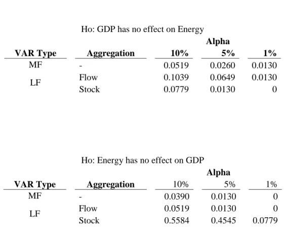
Table 2 displays the proportion of windows that reject the null hypothesis at significance levels 1%, 5% and 10%. Since separate VAR models were conducted for each window, the interpretation is that if a window rejects non-causality, then the conclusion is that in that six year window, there was an observed relationship between the two series. We can see that across both directions of causality, the MF-VAR tends to reject the null hypothesis of non-causality least often. The LF-VAR with flow sampling rejects the null hypothesis that GDP growth does not cause energy consumption growth the most often, with 10.39% of windows rejecting the null at 10% significance, while 7.79% of the LF-VAR with flow sampling windows and 5.19% of the MF-VAR windows indicate direct causality from GDP to energy. Notably, the LF-VAR with stock sampling does not detect causality at 1% significance, although the other two models reject at 1%; however, these highly significant windows do not correspond to the same time period.
The stark contrast between the LF-VAR with flow sampling’s causal predictions from energy consumption to real GDP with the other two models highlights how different aggregation techniques can induce vastly different results. The MF-VAR has a higher power than the LF-VAR, and given that at every significance level, the MF-VAR tends to detect causality at the same amount or fewer windows than the LF-VARs indicates that the aggregation or filtration of monthly energy consumption leads to spurious causal predictions due to compressed
information.
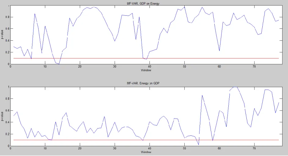
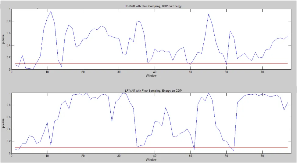
Figures 3-5 display the plotted p-values across the rolling windows for the three models. The plots of p-values for non-causality from real GDP to energy consumption are generally comparable, although the non-causality tests for the LF-VAR with flow sampling does not detect causality around window 40 (1991:Q4 – 1997:Q3) while the tests conducted on the other models result in evidence of a causal relationship. The non-causality tests for energy consumption to real GDP are very different across the three models. P-values for tests resulting from the LF-VAR with flow sampling are typically the largest; the p-values for tests from the LF-VAR with stock sampling are very low, indicating causality in windows 7-49 (1983:Q3 – 1999:Q4); the tests for noncausality stemming from the MF-VAR are somewhere in the middle, indicating the MF-VAR does a better job incorporating all information available from the energy consumption series and generally do not detect evidence of causality from energy consumption to real GDP.
6. Conclusion
bivariate case leads to better predictions about potential causal relationships between real GDP and energy consumption.
Across the three models, there is more evidence of a causal relationship from real GDP to energy consumption. Notably, when there is evidence of a causal relationship from energy consumption to real GDP in the MF-VAR model, 50% of these instances occur in the window directly preceding a window with causality from real GDP to energy. The general consensus in the Granger causality literature is that finding simultaneous causality is the result of issues surrounding timing of data sampling. While it cannot be that the two series contemporaneously influence one another, this finding does suggest that when there is a causal relationship from energy to real GDP, shortly thereafter (ie. across the next window), there does tend to be causality from real GDP to energy consumption, and given that the windows overlap for 22 quarters, there are periods through which the two series influence each other within the overlapping period, known as a feedback loop.
This is in contrast to Salamaliki and Venetis (2013) conclusions. While they conclude that there is a causal relationship in the United States from real GDP to energy, they do not find instances of causality from energy to real GDP, and this may be partially attributable to data aggregation issues.
the early 1990s, and the events of September 11, 2001 coincide with causality from energy to real GDP. This indicates that foreign policy matters might be an unobserved factor leading to the conclusion of a causal relation between the two series.
We could not determine the specific causal mechanism through which these relationships might manifest themselves, nor could we explore causal relationships at higher horizons. Both issues are primarily due to data inadequacies and parameter proliferation. For instance, in order to adopt a trivariate MF-VAR approach with capital stock (sampled annually) as an instrument (as Salamaliki and Venetis (2013)’s use in a LF-VAR setting), we would have to set up a system of 17 equations (12 months of energy consumption, 4 quarters of real GDP, and 1 annual capital stock reading), resulting in 172 parameters per lag. However, given the relatively infrequent instances of causality between the two series (as determined by the noncausality tests based on the MF-VAR), and utilizing the fact that one-step ahead non-causality implies h-step ahead non-causality, we do not believe we would gain much insight in exploring causal relationships at higher time horizons.
While we could only observe direct causality in this study, we have gained valuable insight into the relationship between energy consumption and real GDP, primarily that there are rare instances in which there is such a relationship, and typically direct causality is found from real GDP to energy and not the converse. This observation is important for risk-averse
literature. Furthermore, in those windows during which energy does influence real GDP, it is typically linked to international oil instability. If US lawmakers are interested in conserving energy, they can do so with little influence on US real GDP if they are confident in the capacity for domestic suppliers to meet demand or they are confident in the stability of their relationship with oil rich countries.
References
Akarca, A.T., Long, T.V., 1980. “On the relationship between energy and GNP: a re-examination.” Journal of Energy Development 5, 326–331.
Berndt, E.R., Wood, D.O., 1979. "Engineering and econometric interpretations of energy capital complementarity." American Economic Review 69, 342–354.
Cleveland, C.J., Costanza, R., Hall, C.A.S., Kaufmann, R.K., 1984. "Energy and the US economy: a biophysical perspective." Science 225, 890–897.
Diebold, F 2007. Elements of Forecasting: Fourth Edition. Thomson Higher Education. Mason, Ohio.
Dolado J., Lutkepohl H., 1996. “Making Wald tests work for cointigrated VAR systems.” Econometric Reviews 15, 369-381.
Dufour, J.M., Renault, E., 1998. "Short-run and long-run causality in time series: theory." Econometrica 66, 1099–1125.
Dufour, J.M., Pelletier, D., Renault, E., 2006. "Short run and long run causality in time series: inference." Journal of Economics 132, 337–362.
Foroni, C., Marcellino, M. and Schumacher, C., 2006. “Unrestricted mixed data sampling (MIDAS): MIDAS regressions with unrestricted lag polynomials.” Journal of the Royal Statistical Society: Series A (Statistics in Society), 178: 57–82.
Ghali, K.H., El-Sakka, M.I.T., 2004. "Energy use and output growth in Canada: a multivariate cointegration analysis." Energy Economics 26, 225–238.
Ghysels, E., 2012. “Macroeconomics and the Reality of Mixed Frequency Data,” Working paper, University of North Carolina at Chapel Hill.
Ghysels, E., Santa-Clara, P., Valkanov, R., 2005. “There is a risk-return tradeoff after all.” Journal of Financial Economics 76, 509–548.
Ghysels, E., Sinko, A., Valkanov, R., 2006. “MIDAS regressions: further results and new directions.” Econometric Reviews 26, 53–90.
Ghysels, E., Hill, J. B. and Motegi, K.,2014a. “Granger Causality in Mixed Frequency
Vector Autoregressive Models.” Working Paper, University of North Carolina at Chapel Hill.
Goncalves, S. and Kilian, L. 2004. “Bootstrapping autoregressions with conditional heteroskedasticity of unknown form.” Journal of Econometrics 123, 89-120.
Granger, C.W.J., 1969. “Investigating causal relations by econometric models and cross spectral methods.” Econometrica 37, 424–438.
Granger, C.W.J., 1980. “Testing for causality— a personal viewpoint.” Journal of Economic Dynamics and Control 2, 329–352.
Granger, 1988. "Some recent developments in a concept of causality." Journal of Econometrics 39, 199–211.
Griffin, J.M., Gregory, P.R., 1976. "An intercountry translog model of energy substitution responses." American Economic Review 66 (5), 845–857.
Hill, J.B., 2007. "Efficient tests of long-run causation in trivariate VAR processes with a rolling window study of the money-income relationship." Journal of Applied Econometrics 22, 747–765.
Horowitz, J. and Lobato, I. N. and Nankervis, J. C. and Savin, N. E., 2006. “Bootstrapping the Box–Pierce Q Test: a robust test of uncorrelatedness.” Journal of Econometrics 133, 841-862.
Hudson, E.A., Jorgenson, D.W., 1974. "U. S. energy policy and economic growth," TheBell Journal of Economics and Management Science 5, 461–514.
Jumbe, C., 2004. “Cointegration and causality between electricity consumption and GDP: empirical evidence from Malawi”. Energy Economics 26, 61–68.
Kraft, J., Kraft, A., 1978. “On the relationship between energy and GNP”. Journal of Energy Development 3, 401–403.
Lee, Chien-Chiang. 2006 “The causality relationship between energy consumption and GDP in G-11 countries revisited.” Energy Policy 3, 1086-1093.
Lee, C.C., Chang, C.P., Chen, P.F., 2008. "Energy-GDP causality in OECD countries revisited: the key role of capital stock." Energy Econ. 30, 2359–2373.
Lee, C.C., Chien, M.S., 2010. "Dynamic modelling of energy consumption, capital stock, and real income in G-7 countries." Energy Economics 32, 564–581.
Ljung, G. M., Box, G. E. P., 1978. “On a measure of a lack of fit in time series models.” Biometrika 65, 297-303.
Masih, A.M.M., Masih, R., 1997. "On the temporal causal relationship between energy
consumption, real income, and prices: some new evidence from Asian-energy dependent NICs based on a multivariate cointegration/vector error-correction." Journal of Policy Modeling 19, 417–440.
McCrorie, J.R., Chambers, M.J., 2006. "Granger causality and the sampling of economic processes." Journal of Econometrics 132, 311–336.
Pokrovski, V.N., 2003. "Energy in the theory of production." Energy 28, 769–788.
Salamaliki, P.K., Venetis, I.A. 2013. “Energy consumption and real GDP in G-7: Multi-Horizon causality testing in the presence of capital stock.” Energy Economics, 39, 108-121. Sari, R., Soytas, U., 2007. "The growth of income and energy consumption in six developing
countries." Energy Policy 35, 889–898.
Soytas, U., Sari, R., 2003. “Energy consumption and GDP: causality relationship in G-7 countries and emerging markets.” Energy Economics 25, 33–37.
Sims, C., 1972. "Money, income, and causality." American Economic Review 62, 540–552. Sims, C., 1980. "Macroeconomics and reality." Econometrica 48, 1–48.
Stern, D.I., 1993. "Energy and economic growth in the USA: a multivariate approach." Energy Economics 15, 137–150.
Stern, D.I., 2000. "A multivariate cointegration analysis of the role of energy in the US macroeconomy." Energy Economics 22, 267–283.
Tiao, G. C., 1999. "The ET interview: Professor George C. Tiao." Econometric Theory 15, 389– 424.
Thoma, M., 2004. “Electrical energy usage over the business cycle.” Energy Economics 26, 463– 485.
Toda H.Y., Yamamoto T. 1995. “Statistical inference in vector autoregressions with possibly integrated processes.” Journal of Econometrics 66, 225-250.
Wolf, M., 2000 “Stock returns and dividend yields revisited: a new way to look at an old problem.” Journal of Business and Economic Statistics, 18, 18-30.
Appendix A. Bootstrapping methods overview
Linear time series models generally necessitate that samples come from i.i.d variables; however, it is very rare that autocorrelation between observations are not observed. Time series econometricians have developed various resampling methods to achieve normality of error terms. Bootstrapping is one subset of methods that generally refers to metrics that utilize random sampling with replacement, and can be used to counteract heteroskedasticity, non-normality of errors, etc. In this paper, we consider two methods of bootstrapping, the first is a block-of-block bootstrapping method developed by Horowitz, et al. (2006) and the other is Goncalves and Killian’s (2004) parametric bootstrapping method.
A.1 Horowitz et al (2006)’s Block-of-Block Bootstrapping
This method is based on the Box-Pierce Q-statistic and presents a method of testing whether the first k autocorrelations of a covariance stationary time series are zero in the presence of statistical dependence. The Q statistic approximates a chi-square distribution with a null hypothesis that the series is i.i.d. However, there can be significant inference errors if the null hypothesis is true but the series is statistically dependent. Horowitz et al. note that “time series models that generate uncorrelated but statistically dependent observations have been widely used in economics and finance” and so bootstrapping is an important feature of obtaining reliable p-values.
bootstrapping selection with replacement occurs. A sample is constructed from a sufficiently large number of observations (at least 500), and then the sample is reweighted to account for the fact that some observations were counted multiple times due to the overlapping blocks in the original blocking scheme. Then a Q-statistic is determined, and we use the Ljung-Box test for autocorrelation.
A.2 Goncalves and Kilian (2004) Parametric Bootstrapping
Traditional bootstrapping methods treat regression errors as i.i.d., although conditional heteroskedasticity is a common feature of many macroeconomic and financial time series. However, there is clear evidence that this is rarely true, and so many “non-parametric” bootstrapping methods fail to produce reliable inference testing.
Appendix B. Data Transformation Motivation
Define x(t) = ln(y(t))-ln(y(t-1)) and lny(t) = ln(y(t)). Then, in an AR(1):
𝑥(𝑡) = 𝑎 + 𝑏 ∗ 𝑥(𝑡 − 1) + 𝑒(𝑡), 𝑤ℎ𝑒𝑟𝑒 |𝑏| < 1
b is approximately the growth rate since x(t-1) is defined as lny(t-1). Next, we can write
𝑥(𝑡) = 𝑐 + 𝑢(𝑡),
𝑢(𝑡) = ∑ 𝑏−𝑖𝑒(𝑡 − 𝑖), 𝑤ℎ𝑒𝑟𝑒 𝑖 = 0,1, … ,
𝑎𝑛𝑑 𝑐 = 𝑎
1 − 𝑏
where u(t) is stationary (it does not depend on time t) (Diebold 2007). Notice
𝑙𝑛𝑦(𝑡) − 𝑙𝑛𝑦(𝑡 − 1) = 𝑐 + 𝑢(𝑡) (4.1)
after some algebraic steps, (4.1) reduces to:
𝑙𝑛𝑦(𝑡) = 𝑙𝑛𝑦(0) + 𝑐 ∗ 𝑡 + ∑𝑡−1𝑖=0𝑢(𝑡 − 𝑖) (4.2)
Appendix C. Tables and Figures
Table 1. P-value results for Ljung-Box Portmanteau Test for Autocorrelations
Lag Length
MF-VAR p = 2
Horizon 1 4 8 12
Energy(1) 0.901 0.0225 0.0305 0.0255 Energy(2) 0.7525 0.004 0.026 0.024 Energy(3) 0.8355 0.071 0.092 0.2355
GDP 0.042 0 0 0
p = 3
Horizon 1 4 8 12
Energy(1) 0.5895 0.0645 0.013 0.039 Energy(2) 0.396 0.01 0.069 0.0325 Energy(3) 0.6875 0.0405 0.203 0.121
GDP 0.294 0 0 0
Lag Length Lag Length
LF-Flow p = 2 LF-Stock p = 2
Horizon 1 4 8 12 Horizon 1 4 8 12
Energy 0.799 0.0015 0.004 0.0265 Energy 0.6625 0.0495 0.138 0.1075
GDP 0.0185 0 0 0 GDP 0.0215 0 0 0
p = 3 p = 3
Horizon 1 4 8 12 Horizon 1 4 8 12
Energy 0.4225 0.0015 0.0045 0.022 Energy 0.6285 0.021 0.2175 0.1415
Table 2. Rejection rates for each model at various significance levels: the proportion of windows that reject the null hypothesis
Ho: GDP has no effect on Energy
Alpha
VAR Type Aggregation 10% 5% 1%
MF - 0.0519 0.0260 0.0130
LF Flow 0.1039 0.0649 0.0130
Stock 0.0779 0.0130 0
Ho: Energy has no effect on GDP
Alpha
VAR Type Aggregation 10% 5% 1%
MF - 0.0390 0.0130 0
LF Flow 0.0519 0.0130 0
Figure 1. Annual Quarterly Real GDP Growth, 1982-20061
Notes:
Figure 2. Annual Monthly Energy Consumption Growth, 1982-2006
Notes:
Figure 3. Plotting of p-values from rolling window analysis of Mixed Frequency VAR
Notes:
Red line indicates p-value threshold of 0.10.
Figure 4. Plots of p-values from rolling window analysis of the Low Frequency VAR with flow sampling
Notes:
Red line indicates p-value threshold of 0.10.
Figure 5. Plots of p-values from rolling window analysis of the Low Frequency VAR with stock sampling
Notes:
Red line indicates p-value threshold of 0.10.