Abstract— The cost contingency estimation is an essential phase in the risk management, especially when the regime of performance is stochastic. This research proposes a probabilistic model to estimate project cost contingency by considering the fact that any risk can occur on a variety of values in terms of economic impact. The impact of risks on the project is achieved by qualitative analysis through three parameters: schedule, cost, and performance. In addition, a stochastic quantitative analysis has been performed using Monte Carlo Simulation (MCS) with the aim to determine the probability distribution of the contingency cost and the related level of risk coverage. The proposed method has been applied on a construction project of a real life company using @Risk for Excel software. By obtaining the contingency amount for the project, it can be realized that with allocating a determined budget, a specific level of risks can be covered and vice versa. Eventually, the robustness of the result was evaluated by another probability distribution to compare the obtained results.
Index Terms—Cost Contingency Estimation, Monte Carlo Simulation, Project Management, Risk Analysis, Stochastic Regime.
I. INTRODUCTION
OST contingency assessment is one of the most significant subjects in the project management to find out the more accurate cost amount to allocate in the projects [13], [3], [18], and [23].
Commonly, in the traditional methods, the risk occurrence probability and related percentages were used to estimate the contingency fund [1][21], [21]. Some authors presented reasons such as inaccurate, complex and inordinate allocation of budget to refuse using traditional methods [14], [16], [2], [19], [24]. Reference [2] prepared the cost contingency estimation methods such as Monte Carlo Simulation [17], [10], method of moments [11], fuzzy sets [22], and artificial neural networks [9], [25]. Nevertheless, some of these strategies such as artificial neural networks and fuzzy sets involved the problem of complexity and uncertainty for estimation of contingency costs [15]. Reference [23] presented
Fahimeh Allahi is Ph.D. student of DIME, Department of Polytechnic, University of Genoa, Genoa, Italy (phone: 00393920345718; e-mail: allahi@ dime.unige.it).
Lucia Cassettari is the professor of DIME, Department of Polytechnic, University of Genoa, Genoa, Italy (e-mail: [email protected]).
Marco Mosca is the visiting professor of DIME, Department of Polytechnic, University of Genoa, Genoa, Italy (e-mail: [email protected]).
that the accurate cost contingency amount can be obtained by probabilistic methods. Among probabilistic methods, MCS is one of the most common method, which is applied for cost contingency estimation and risk analysis in construction projects [4]. Furthermore, in comparison with other methods, MCS is more impressive because of comprehensible, easy to use and feasible [12]. Besides, [6] presented that the results in a stochastic regime are more accurate in comparison with the deterministic regime. According to literature, this research proposed a method to estimate the contingency in stochastic regime by MCS. The purpose is to support the Companies with the stochastic regime against the risk of cost overruns to win in the tenders.
The early methodological phases of a qualitative and quantitative risk analysis are presented in the next section. Then, the method is applied to an industrial project for a real life company operating in the field of railway signaling and integrated transport systems. After a critical risk analysis, the robustness of results is checked by another probability distribution and finally, the Authors draw conclusion on the research.
II. RISK IDENTIFICATION: QUALITATIVE AND QUANTITATIVE ANALYSIS
Risk identification is one of the important steps to recognize whole risks, which can affect the project budget. In order to identify these risks, the company uses a checklist guide. It makes possible to identify different kinds of risks: those of a strictly operational nature and those of a legal/financial nature arising from contract terms. The checklist was filled out with some interviews dedicated to members of the company, directly have involved in the management of the project. Qualitative and quantitative assessment are applied after the risk identification. The qualitative analysis determines the significant risks for the step of mitigate action.
In this research, the impacts that the risks may have on the project are qualitatively identified through the three parameters: schedule, cost and performance. For each of these, it is necessary to define a scale to be able to identify a high (3), medium (2) or low (1) impact. The indicator used to rank the risks is the "risk factor", which is obtained by the multiplication of the probability occurrence of the mentioned risks by the level of their severity. Regarding the impact on schedule parameter, there are two types of risks, namely operational and legal/financial. Therefore, it is necessary to define two different scales for the two types of risk.
Fahimeh Allahi, Lucia Cassettari, Marco Mosca
Stochastic Risk Analysis and Cost Contingency
Allocation Approach for Construction Projects
Applying Monte Carlo Simulation
According to operational risks, Table I presents the number of delayed days on the project completion, caused by the occurrence of the risk. It proposes for the delay more than 30 days, the severity of risk will be high and influences on the cost of the project.
Table I Scale for operational risks
IMPACT ON THE SCHEDULE PARAMETER
Number of delayed days Severity
≤ 7 days (1)
(2) (3) 7-30 days
≥ 30 days
[image:2.612.62.283.299.396.2]As regards to the legal/financial risks relating to the payment of the penalties for late delivery, the scale of Table II is considered.
Table II Scale for legal/financial risks
IMPACT ON THE SCHEDULE PARAMETER
Payment Action Severity
< 15 days ≥ 15 days
Penalty clauses not applied Penalty clauses applied
for every late day
(1) (3)
This table clearly shows that as long as the request subject to a contract penalty has a delay lower than of 15 days, the associated penalty is not actually applied and hence not considered. Obviously, once 15 days are reached, every day of delay accrued will be paid.
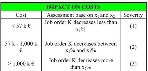
For analyzing the impact on costs, a single scale is considered for both types of risk (Table III). The assessment is closely related to the fact that the risk occurrence would result in a more or less significant decrease in the cost of the project K or in the Gross Margin. Based on several studies, values x1 and x2 were identified as discriminants between the various levels of impact (not reported due to corporate intellectual property right).
Table III Scale for impact on cost
IMPACT ON COSTS
Cost Assessment base on x1 and x2 Severity < 57 k € Job order K decreases less than x1% (1)
57 k - 1,000 k €
Job order K decreases between
x1% and x2% (2)
> 1,000 k € Job order K decreases more than x2% (3)
Besides, the impact on performance, it is not necessary to apply separate analyses for the two types of risk. The scale used in this case is presented in Table IV.
[image:2.612.311.570.518.587.2]
Table IV Scale for impact on performance
IMPACT ON PERFORMANCE
Performance Severity
The system/component does not meet contract specification and operational inefficiency of it exists.
A specific requirement is not satisfied without negative consequences on system’s operational performance (Visible risk to the customer). Contract requirements not fully satisfied (Not visible risk to the customer).
(3)
(2)
(1)
Once the mentioned scales were defined, the scale related to Risk Occurrence Probability (ROP) is determined. In particular, ROP is evaluated according to the followed criteria.
• ROP < 20%: Severity of risk = 1; • 20% ≤ ROP ≤ 50%: Severity of risk = 2; • ROP > 50%: Severity of risk = 3.
In order to rank the risks, the risk factor obtains by combining the qualitative assessments of the severity of the risks and its probability of occurrence in a matrix that presents a numeric value. The latter is calculated by multiplying the probability parameter by the impact parameter (in quantifying the impact, the highest value among those recorded for schedule, cost and performance was considered). The possible risk factor values are summarized in Table V.
Table V Risk factors values
probability of occurrence
3 3(●) 6 (*) 9 (*)
2 2 (◊) 4(●) 6 (*)
1 1 (◊) 2 (◊) 3(●)
1 2 3
Risk Impact
The obtained risk factor makes it possible to rank the identified risks according to priority. In particular, it was decided to proceed with the next step of analysis only for the risks characterized by a risk factor greater than or equal to three (The symbols of (●) and (*) that are determined in Table V).
The economic impact of the possible occurrence of the risk will be quantified as the next step.
[image:2.612.46.301.593.716.2]impact is estimated as the product of the accrued delay (typically assumed greater than or equal to 15 days) by the sum of the penalties.
Once the values of the impact associated with the individual risks are determined, the possible mitigation actions are implemented by identified precaution for each of them. This activity is based on an analysis of the causes generating the individual risks and aims at reducing/eliminating the impact of the risk.
It should be noted that the implementation of a mitigating action allows the reduction of an uncertain cost with a certain incurred cost (the cost of the action) whose amount is estimated to be lower. In order to ensure the right balance between risk reduction and cost-effectiveness, it is necessary to determine the net benefit of the mitigating actions. This benefit is determined as the difference between the expected value of the risk before and after the risk mitigating action. Clearly only the interventions with a positive net benefit must be implemented, unless there is still an overall benefit for the project and/or the Company.
After the reassessment of the residual risks and their final impact value, the amount of contingency fund will be defined. The set aside amount, makes it possible to "cover" the project if the risk event occurs. The objective is to minimize the occurrence of extra costs associated with the occurrence of the risk while trying at the same time to minimize the impact of the overheads that reduce the competitiveness of the job offer. In particular, the choice of the percentage of contingency to be allocated is a function of the value of the risk occurrence probability, according to the criteria in Table VI.
Table VI Contingency allocation policy
CONTINGENCY
Prob ≥50% Contingency = Whole impact value 20%<Prob<50% Contingency = 50% of the impact value
Prob ≤ 20% Contingency = 30% of the impact value
After starting the described process, all the risks that did not occur should be reviewed to possibly re-determine the associated contingency cost.
Finally, when checking the condition that makes it possible to declare the risk "closed", the associated contingency reserve can be:
• "Used": if the risk has occurred, causing economic damage to the project. The contingency is considered "used" to cover the damage suffered up to a maximum value equal to the amount previously allocated. Any part of the damage that is not covered by the contingency is to be considered an "extra cost".
• "Releasable" or "Partially Releasable": in case the risk event does not occur and causing fewer damages compared to the allocated contingency.
In order to monitor the occurrence of the event linked to the risk, specific milestones must be assigned to the activities
associated with the risk event. The completion of the milestone indicates that the risk, which has or has not occurred in the past, will not occur in the future. It is clear that a monitoring and a complete and comprehensive review of the risks must necessarily cover the entire project, which hence be constantly updated throughout its life cycle.
III. STOCHASTICQUANTITATIVEANALYSIS The quantitative analysis described above is based on the assumption that the expected value of the risk and calculated as the product of the occurrence probability and the economic impact. It is enough to capture the essential aspects of the overall risk profile of the project.
However, since the regime of normal operations of companies is not deterministic but stochastic, it is necessary to take into account the fact that any risk can occur on a variety of values in terms of economic impact. Precisely for this reason, the methodology described above has been integrated with the steps illustrated below. For each risk, the decision maker identifies a probability distribution associated with the values of severity of the economic impact of the event. Among the most widely used, it suffices to mention uniform distribution, triangular distribution, normal distribution and beta distribution. The @Risk for Excel software is used for quick and easy definition of probability distributions, simply by selecting and customizing templates used in the paper.
Using the Monte Carlo method allows for the distribution of the overall likelihood of the contingency fund to be allocated starting from the probability distributions attributed to the individual risks. In the next part, the application to a railway construction project is carried out. Once the simulation runs, the curve of the probability distribution of the contingency and its integral curve is illustrated by means of MCS.
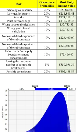
IV. APPLICATION TO A CONSTRUCTION PROJECT The obtained results from the application of the methodology described to a construction project in the railway sector are illustrated in Table VII. Once the critical risks were selected in section three (for risk factor > 3), each risk was associated with an appropriate probability distribution.
Table VII Analyzed risk list
Risk Occurrence Probability impact value Most likely
Technological maturity 20% €20,872.07
Low quality supply 20% €251,841.41
Reworks 5% €174,311.15
Plant software bugs 10% €176,216.38 Wrong structural calculation 10% €37,733.33
Wrong geotechnical
calculation 10% €37,733.33
Not consolidated experience
of the subcontractor 10% €226,400.00 Not consolidated experience
of the subcontractor 10% €226,400.00 Failure to define supply
boundaries among
subcontractors 10% €75,466.67
Passing the maximum number of acceptable
breakdowns. 5% €550,996.39
[image:4.612.47.300.72.506.2]Possible breakdowns 20% €402,488.89
Fig. 1 Beta distribution used for the "technological maturity" risk
At this step of the methodological analysis, it is important to carry out a number of experimental runs on the model such that it is possible to obtain an output of statistically reliable results with a known confidence level. For this purpose, the methodology of the Mean Square Pure Error in repeated run which was developed by [7], [8] was used to determine the correct number of simulation runs. The proposed approach is based on the analysis of the curves illustrating the trend of the quantities Mean Square Pure Error of the Mean (MSPEMED) and Mean Square Pure Error of the Standard Deviation (MSPESTDEV). This methodology was created by the
[image:4.612.324.576.228.398.2]Authors as a conceptual extension for the Monte Carlo simulators evolving over time [20]. In addition, significantly by using the MSPE method, the experimental error in the results was controlled [5]. To this end, an experimental campaign of 5 simulations, each representing a sample of 20,000 elements, was set. The trend curves of the Mean Square Pure Error of the Mean and Standard Deviation shown in Fig. 2 put in evidence that both curves stabilized at around 20,000 runs. It presents for this number of runs the mean value of the output will be very stable and the contribution of these two variables on the confidence interval of the contingency fund will be almost negligible.
Fig. 2 Trend of the quantities MSPEMED and MSPESTDEV depending on the number of runs
Once 20,000 is set as the number of repeated simulation runs, the curve of the probability distribution of the contingency and its integral curve, shown in Fig. 3 and Fig. 4 were obtained.
Fig. 3 Probability distribution of contingency cost MSPE Med
[image:4.612.321.558.516.659.2]Fig. 4 cumulative probability curve of contingency cost
This Monte Carlo analysis makes it possible to determine the probability distribution of the contingency cost and allows identifying the degree of coverage corresponding to each value of the total allocated contingency fund.
obtained by integration of the probability distribution Fig. 3 and features the possible contingency values on the X axis and the "Level of Coverage" on the Y axis (
Hence, The Level of Coverage is the probability of being able to cover completely the costs arising from the occurrence of the risks using a set total amount of allocated contingency reserve.
The probability distribution in Fig.
contingency tends to spread according to a normal pattern. In addition, the most probable value of the distribution by a confidence level of (1 - α) % with α = 0.05 is be
600,000 and 700,000 €. Consequently, the data can be considered highly stable. In the Table VII
probability values are lower than or equal to
to Table VI, contingency for Prob ≤ 20% equals to 30% of the impact value. Hence, the estimated contingency under a deterministic system was equivalent to 654,138
the most likely impact values of the individual risks multiplying by 0.3). By analyzing the cumulative probability curve (Fig. 4), it may be noted that by a coverage level of 90 %, the contingency cost is equal to 690 € which totally covers the risks. In particular, entering the contingency value resulted from Table VII (654,138 €), it can be obtained a risk coverage probability of about 40%. It presents that this graph does not provide information concerning the value of the extra costs but only concerning the level of risk coverage implemented with a 30% of contingency set aside for risks with a probability of occurrence of no more than 20% (see Table VII
allocating € 500,000 would be equal to take on a level of coverage of zero against the risk of extra costs. The same level of risk coverage would be obtained also by setting aside a contingency equal to zero, but it is clear that, in both cases, the extra costs incurred would be significantly different.
cumulative probability curve of contingency cost
his Monte Carlo analysis makes it possible to determine the probability distribution of the contingency cost and allows responding to each value of the total allocated contingency fund. The curve is obtained by integration of the probability distribution from and features the possible contingency values on the X axis and the "Level of Coverage" on the Y axis (Fig. 4). Hence, The Level of Coverage is the probability of being able to cover completely the costs arising from the occurrence of the risks using a set total amount of allocated contingency Fig. 3 presents the contingency tends to spread according to a normal pattern. In addition, the most probable value of the distribution by a α) % with α = 0.05 is between the onsequently, the data can be VII, the occurrence 20 and according ≤ 20% equals to 30% of the impact value. Hence, the estimated contingency under a nt to 654,138 € (the sum of the most likely impact values of the individual risks multiplying by 0.3). By analyzing the cumulative probability be noted that by a coverage level of 90 € which totally covers the risks. In particular, entering the contingency value resulted €), it can be obtained a risk coverage probability of about 40%. It presents that this graph does not provide information concerning the value of the extra costs but only concerning the level of risk coverage implemented with a set aside for risks with a probability of VII). Furthermore, € 500,000 would be equal to take on a level of rage of zero against the risk of extra costs. The same level of risk coverage would be obtained also by setting aside a contingency equal to zero, but it is clear that, in both cases, the extra costs incurred would be significantly different.
V.ROBUSTNESS ANALYSIS OF THE METHO
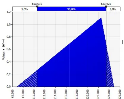
[image:5.612.340.549.135.302.2]In order to evaluate the robustness of the identified results, it was decided to use other probability distributions for the characterization of the risks and then compare the obtained results.
Fig. 5 Triangular distribution used for the "technological maturity" risk
Therefore, triangular distributions were chosen instead of the beta distributions (
maintaining the min, max and most likely values as the supposed data.
According to the proposed method, five simulations were performed, each having a number of 20,000 repeated r
[image:5.612.328.566.456.614.2]the trend curves of MSPEMED and MSPESTDEV were built.
Fig. 6 Trend of the quantities MSPEMED and MSPESTDEV depending on the number of runs
As the graph in Fig. 6 shows, while the curve of MSPEMED stabilizes at 20,000 runs, the curve relating to MSPESTDEV still shows phenomena of instability so that it would be necessary to increase the number of Monte Carlo runs, namely the sample size.
MSPE Med
NALYSIS OF THE METHODOLOGY In order to evaluate the robustness of the identified results, it was decided to use other probability distributions for the characterization of the risks and then compare the obtained
Triangular distribution used for the "technological maturity"
Therefore, triangular distributions were chosen (Fig. 5) instead of the beta distributions (Fig. 1), because of maintaining the min, max and most likely values as the According to the proposed method, five simulations were performed, each having a number of 20,000 repeated runs, and the trend curves of MSPEMED and MSPESTDEV were built.
Trend of the quantities MSPEMED and MSPESTDEV depending on the number of runs
shows, while the curve of MSPEMED stabilizes at 20,000 runs, the curve relating to MSPESTDEV still shows phenomena of instability so that it would be necessary to increase the number of Monte Carlo
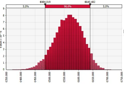
By using a sample of 20,000 runs, the probability distribution and probability curve of the contingency cost (Fig. 7 and Fig. 8) were obtained. Fig. 7 shows how the mean value of the distribution drops to € 565,403, with a confidence band of (1-α)% with α = 0.05.
[image:6.612.50.299.125.296.2]
Fig. 7 Probability distribution contingency with triangular distributions
[image:6.612.48.298.424.591.2]The analysis of the cumulative probability curve is shown in Fig. 8. By the contingency amount of 654,138 € (the obtained result from the deterministic analysis), a level of risk coverage of 90% is obtained which is higher than the determined amount using beta distribution.
Fig. 8 cumulative probability curve of contingency with triangular distributions
The comparison between the captured results by two different types of probability distributions, while maintaining the min, max and most likely values unchanged, shows the obtained contingency amount covers the determined risks up to 40% probability. Hence, by analyzing both of Fig. 4 and Fig. 8, the contingency amount of 690 € covers the total obtained risk with the coverage level up to 90%.
VI. CONCLUSIONS AND FUTURE RESEARCH
The proposed method considered the qualitative risk analysis and stochastically quantitative analysis by using the Monte Carlo method. In addition, the application for a real life company executed for two probability distributions, which presented the cost contingency amount to allocate in the project. The presented method is powerful as it can show the contingency amount for the risks happening with the determined probability (under 20 percent) and estimates the contingency value to cover all the possible risks.
The comparison between the results obtained from two different types of probability distributions showed two different coverage level for one contingency amount, which means the contingency value, is not accurate. In addition, the result was influenced by the choices of the decision-maker. Therefore, it is resulted that the method has the problem of subjective and inaccurate. Besides, by this method the companies can evaluate the contingency cost by the determined coverage. It allows to easily managing the budget of the project base on the results.
As a future work, the proposed method can be more accurate and have the feature of objective. By assigning the risk assessment to another project manager in order to estimate carefully.
REFERENCES
[1] I. Ahmad, “Contingency allocation: a computer-aided approach”, AACE Transactions Conf., 28 June 1992, Orlando, F.4, pp. 1-7.
[2] D. Baccarini, “Estimating Project Cost Contingency – Beyond the 10% syndrome”, Australian Institute of Project Management National Conf., Nov. 2005, Victoria: Australian Institute of Project Management. [3] D. Baccarini, P.E.D. Love, “Statistical Characteristics of Cost
Contingency in Water Infrastructure Projects”, Journal of Construction Engineering and Management, vol. 140, no. 3, 2014.
[4] P. Bakhshi, A. Touran "An overview of budget contingency calculation methods in construction industry." Proceed Engineering J., vol. 85, pp. 52-60, 2014.
[5] I. Bendato, L. Cassettari, P.G. Giribone, R. Mosca, “Monte Carlo method for pricing complex financial derivatives: An innovative approach to the control of convergence”, J. of Applied Mathematical Sciences, vol. 9, no. 124, pp. 6167-6188, 2015.
[6] I. Bendato, L. Cassettari, M. Mosca, R. Mosca, “Stochastic techno-economic assessment based on Monte Carlo simulation and the Response Surface Methodology: The case of an innovative linear Fresnel CSP (concentrated solar power) system”, Journal of Energy, vol. 101, pp. 309-324, 2016.
[7] L. Cassettari, P.G. Giribone, M. Mosca, R. Mosca, “The stochastic analysis of investments in industrial plants by simulation models with control of experimental error: Theory and application to a real business case” Journal of Applied Mathematical Sciences, vol. 4, no.76, pp. 3823–3840, 2010.
[8] L. Cassettari, R. Mosca, R. Revetria, “Monte Carlo Simulation Models Evolving in Replicated Runs: A Methodology to Choose the Optimal Experimental Sample Size”, Journal of Mathematical Problems in Engineering, Vol. 2012, pp. 0-17, 2012.
[9] D. Chen, F.T. Hartman, “A neural network approach to risk assessment and contingency allocation”, AACE Transactions Conf., June 2000, pp. 1-6.
[10] D.E. Clark, “Monte Carlo Analysis: ten years of experience”. Journal of Cost Engineering, vol. 43, no. 6, pp. 40-45, 2001.
[12] I.A. Eldosouky, A.H. Ibrahim, H.E. Mohammed, “Management of construction cost contingency covering upside and downside risks.”
Alexandria Eng. J., vol.53, no. 4, pp. 863–881, 2014.
[13] M.W. Hammad, A. Abbasi, M.J. Ryan, “Allocation and Management of Cost Contingency in Projects”, Journal of Management in Engineering, vol. 32, no. 6, 2016.
[14] F. T. Hartman, “Do not park your brain outside”, Upper Darby PA: PMI, 2000.
[15] D. Howell, C. Windahl, R. Seidel, “A project contingency framework based on uncertainty and its consequences”, International Journal of Project Management, vol. 28, pp. 256–264, 2010.
[16] A.M.G. Khalafallah, E.S.M. Taha, “Estimating Residential Projects Cost Contingencies Using a Belief Network”, Conference of Project Management: Vision for Better Future, 2005, Cairo, Egypt, Dec. 2007, to be published.
[17] R.B. Lorance, R.V. Wendling, “Basic techniques for analyzing and presenting cost risk analysis”, AACE Transactions, Risk, vol. 1, pp. 1-7, 1999.
[18] P.E.D. Love, C.P. Sing, B. Carey, J.T. Kim, “Estimating Construction Contingency: Accommodating the Potential for Cost Overruns in Road Construction Projects”, Journal of Infrastructure Systems, vol. 21, no. 2, 2015.
[19] S. Mak, D. Picken, “Using risk analysis to determine construction project contingencies”, Journal of Construction Engineering and Management, vol. 126, no. 2, pp. 130-136, 2000.
[20] R. Mosca, L. Cassettari, R. Revetria, “Experimental Error Measurement in Monte Carlo Simulation”, Abu-Taieh, E.M.O, El Sheikh, A.A.R.,
Handbook of Research on Discrete Event Simulation Environments: Technologies and Applications, Information Science Reference, Hershey, New York, USA, 2010.
[21] O. Moselhi, “Risk assessment and contingency estimating”, American Association of Cost Engineers (AACE) Transactions Conf., 13-16th July 1997, Dallas, pp. 1-6.
[22] J. H. Paek, Y. W. Lee, J. H. Ock, “Pricing Construction Risk: Fuzzy Set Application”, Journal of Construction Engineering and Management, vol. 119, no. 4, pp.743-756, 1993.
[23] A. Salah, O. Moselhi, “Contingency modelling for construction projects using fuzzy-set theory”, Journal of Engineering, Construction and Architectural Management, vol. 22, no. 2, pp. 214-241, 2015.
[24] P. A. Thompson, J. G. Perry, “Engineering construction risks”, Thomas Telford Conf., London, 1992.