Abstract— Kumaraswamy Kumaraswamy distribution was obtained by compounding two Kumaraswamy random variables. In this paper, homogenous ordinary differential equations (ODES) of different orders were obtained for the probability density function, quantile function, survival function and hazard function of Kumaraswamy Kumaraswamy distribution. This is possible since the aforementioned probability functions are differentiable. Differentiation and modified product rule were used to obtain the required ordinary differential equations, whose solutions are the respective probability functions. The different conditions necessary for the existence of the ODEs were obtained and it is almost in consistent with the support that defined the various probability functions considered. The parameters that defined each distribution greatly affect the nature of the ODEs obtained. This method provides new ways of classifying and approximating other probability distributions apart from Kumaraswamy Kumaraswamy distribution considered in this research.
Index Terms— Differentiation, product rule, quantile
function, survival function, approximation, hazard function.
I. INTRODUCTION
ALCULUS is a very key tool in the determination of mode of a given probability distribution and in estimation of parameters of probability distributions, amongst other uses. The method of maximum likelihood is an example.
Differential equations often arise from the understanding and modeling of real life problems or some observed physical phenomena. Approximations of probability functions are one of the major areas of application of calculus and ordinary differential equations in mathematical statistics. The approximations are helpful in the recovery of the probability functions of complex distributions [1-4].
Apart from mode estimation, parameter estimation and approximation, probability density function (PDF) of probability distributions can be expressed as ODE whose
Manuscript received December 9, 2017; revised January 15, 2018. This work was sponsored by Covenant University, Ota, Nigeria.
H. I. Okagbue, P.E. Oguntunde and A. A. Opanuga are with the Department of Mathematics, Covenant University, Ota, Nigeria.
[email protected] [email protected]
[email protected] P. O. Ugwoke is with the Department of Computer Science, University of Nigeria, Nsukka, Nigeria and Digital Bridge Institute, International Centre for Information & Communications Technology Studies, Abuja, Nigeria
solution is the PDF. Some of which are available. They include: beta distribution [5], Lomax distribution [6], beta prime distribution [7], Laplace distribution [8] and raised cosine distribution [9].
The aim of this research is to develop homogenous ordinary differential equations for the probability density function (PDF), Quantile function (QF), survival function (SF) and hazard function (HF) of Kumaraswamy Kumaraswamy distribution. The ODE for the invese survival function and reversed hazard function (RHF) of the distribution are complex and not included in the paper. This will also help to provide the answers as to whether there are discrepancies between the support of the distribution and the necessary conditions for the existence of the ODEs. Similar results for other distributions have been proposed, see
[10-22] for details. Kumaraswamy Kumaraswamy distribution was obtained
by compounding two Kumaraswamy random variables. It is one of the interval bounded support probability distributions. The distribution was proposed by El-Sherpieny and Ahmed [23] and generalized by Mahmoud et al. [24]. Also, Ahmed et al. [25] proposed the Kumaraswamy Kumaraswamy Weibull distribution as an improved model over the parent distributions. The boundary properties and notes of the distribution were discussed extensively in Okagbue et al. [26] and Hamedani [27]. The ordinary differential calculus was used to obtain the results.
II. PROBABILITY DENSITY FUNCTION
The probability density function of the Kumaraswamy Kumaraswamy is given as;
1
1 1
1
( )
(1
)
1 (1
)
1
1 (1
)
a
b a
f x
ab
x
x
x
x
(1)To obtain the first order ordinary differential equation,
differentiate equation (1). The probability density function is broken into distinct
components to ease the differentiation.
( )
f x
ab
ABCD
(2)Classes of Ordinary Differential Equations
Obtained for the Probability Functions of
Kumaraswamy Kumaraswamy Distribution
Hilary I. Okagbue,
IAENG
, Pelumi E. Oguntunde, Abiodun A. Opanuga and Paulinus O. Ugwoke
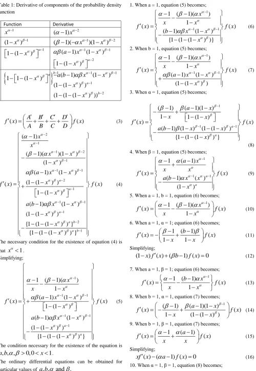
Table 1: Derivative of components of the probability density function
Function Derivative
A 1
x
(
1)
x
2B 1
(1
x
)
(
1)(
x
1)(1
x
)
2C 1
1 (1
x
)
a
1 12
(
1)
(1
)
1 (1
)
aa
x
x
x
D
11
1 (1
)
b a
x
1 11 2
(
1)
(1
)
(1 (1
) )
(1 (1 (1
) ))
ab
a b
x
x
x
x
( )
A
B
C
D
( )
f x
f x
A
B
C
D
(3)2 1 1 2 1 1 1 2 1 1 1 1 2 1
(
1)
(
1)(
)(1
)
(1
)
(
1)
(1
)
(1 (1
) )
( )
1 (1
)
(
1)
(1
)
(1 (1
) )
{1 (1 (1
) ) }
{1 (1 (1
) ) }
a a a a b a b
x
x
x
x
x
a
x
x
x
f x
x
a b
x
x
x
x
x
( )
f x
(4)The necessary condition for the existence of equation (4) is that
x
1
. Simplifying;1
1 1
1 1
1
1
(
1)(
)
1
(
1)
(1
)
( )
( )
1 (1
)
(
1)
(1
)
(1 (1
) )
{1 (1 (1
) ) }
a a
x
x
x
a
x
x
f x
f x
x
a b
x
x
x
x
(5)The condition necessary for the existence of the equation is
, , ,
0,0
1
a b
x
. The ordinary differential equations can be obtained for
1. When a = 1, equation (5) becomes;
1
1 1
1
(
1)(
)
1
( )
( )
(
1)
(1
)
{1 (1 (1
) )}
x
x
x
f x
f x
b
x
x
x
(6)2. When b = 1, equation (5) becomes;
1
1 1
1
(
1)(
)
1
( )
( )
(
1)
(1
)
(1 (1
) )
x
x
x
f x
f x
a
x
x
x
(7)3. When α = 1, equation (5) becomes;
1
1 1
(
1)
(
1)(1
)
1
1 (1
)
( )
( )
(
1) (1
)
(1 (1
) )
{1 (1 (1
) ) }
a aa
x
x
x
f x
f x
a b
x
x
x
(8) 4. When β = 1, equation (5) becomes;1
1 1
1
(
1)
( )
( )
(
1)
(
)
(1
)
a a
a
x
x
x
f x
f x
a b
x
x
x
(9)5. When a = 1, b = 1, equation (6) becomes;
1
1
(
1)(
)
( )
( )
1
x
f x
f x
x
x
(10)6. When a = 1, α = 1; equation (6) becomes;
1
(
1)
( )
( )
1
1
b
f x
f x
x
x
(11) Simplifying;(1
x f x
)
( ) (
b
1) ( )
f x
0
(12) 7. When a = 1, β = 1; equation (6) becomes;
1
1
(
1)
( )
( )
1
b
x
f x
f x
x
x
(13)8. When b = 1, α = 1, equation (7) becomes;
1
(
1)
(
1)(1
)
( )
( )
1
(1 (1
) )
a
x
f x
f x
x
x
(14)9. When b = 1, β = 1, equation (7) becomes;
1
(
1)
( )
a
( )
f x
f x
x
x
(15) Simplifying;( ) (
1) ( )
0
1
(
1)
( )
( )
(1
)
a aa
a b
x
f x
f x
x
x
x
(17) 11. When a = 1, b = 1, α = 1, equation (10) becomes;1
( )
( )
1
f x
f x
x
(18) Simplifying;(1
x f x
)
( ) (
1) ( )
f x
0
(19) 12. When a = 1, b = 1, β = 1, equation (10) becomes;1
( )
( )
f x
f x
x
(20) Simplifying( ) (
1) ( )
0
xf x
f x
(21)13. When b = 1, α = 1, β = 1, equation (14) is the same with equation 205;
1
( )
a
( )
f x
f x
x
(22) Simplifying( ) (
1) ( )
0
xf x
a
f x
(23)III. QUANTILE FUNCTION
The Quantile function of the Kumaraswamy Kumaraswamy is given as;
1 1 1 1
( )
1
1
1 (1
)
a b
Q p
p
(24)
In order to obtain the first order ordinary differential equation for the Quantile function of the Kumaraswamy
Kumaraswamy distribution, differentiate equation (24);
1 1 1
1 1
1
1 1 1
1 1
1
1 1
1
( )
(1
)
1
1 (1
)
1
1
1 (1
)
1 (1
)
a
b b
a a
b b
Q p
p
p
ab
p
p
(25)
Equation can be simplified using equation (24) to obtain;
1
1 1
1 1 1
1 1 1 1
1
1 1
1 1 1
(1
)
1 (1
)
1
1 (1
)
1
1
1 (1
)
( )
(1
) 1 (1
)
1
1 (1
)
1
1
1 (1
)
a a
b b b
a b
a
b b
a b
p
p
p
p
Q p
ab
p
p
p
p
(26) The necessary condition for the existence of equation is that:
, , ,
0,0
1
a b
p
. The following equations obtained from equation (24) areneeded in the simplification of equation (26).
1 1 1
( ) 1
1
1 (1
)
a b
Q
p
p
(27)
1 1 1
1
( )
1
1 (1
)
a b
Q
p
p
(28)
1 1
(1
( ))
1
1 (1
)
a b
Q
p
p
(29)1 1
1 (1
( ))
1 (1
)
a b
Q
p
p
(30)1
[1 (1
Q
( )) ]
p
a
1 (1
p
)
b (31)1
1 [1 (1
Q
( )) ]
p
a
(1
p
)
b (32)(1 [1 (1
Q
( )) ] )
p
a b
1
p
(33) Substitute equations (24) (27)-(33) into equation (26) to
1
1 (1
( ))
1 (1
( ))
1
( )
( )
( )
1
1 (1
( ))
1 (1
( ))
1
( )
( )
a
b a
a
Q
p
Q
p
Q
p Q p
Q p
ab
Q
p
Q
p
Q
p
Q
p
(34) Simplify equation (34);
1
1 1 1
1
1 (1
( ))
1 (1
( ))
1
( )
( )
( )
b a
a
Q
p
Q
p
Q
p
Q
p
Q p
ab
(35) The ordinary differential equations can be obtained for particular values of
a b
, , and .
Special cases 1. When a = 1, equation (35) becomes;
1
1 1(1
( ))
1
( )
( )
( )
b
Q
p
Q
p
Q
p
Q p
b
(36) 2. When b = 1, equation (35) becomes;
1
1 11 (1
( ))
1
( )
( )
( )
a
Q
p
Q
p
Q
p
Q p
a
(37) 3. When α = 1, equation (35) becomes;
1
1
11
1 (1
( ))
1 (1
( ))
1
( )
( )
b a
a
Q p
Q p
Q p
Q p
ab
(38) 4. When β = 1, equation (35) becomes;
1
1 11 (
( ))
( )
( )
( )
b a
a
Q
p
Q
p
Q
p
Q p
ab
(39) 5. When a = 1, b = 1, equation (36) becomes;
1 11
( )
( )
( )
Q
p
Q
p
Q p
(40)6. When a = 1, α = 1; equation (36) becomes;
1
1(1
( ))
1
( )
( )
b
Q p
Q p
Q p
b
(41)7. When a = 1, β = 1; equation (36) becomes;
1 1
1
( )
( )
( )
b
Q
p
Q
p
Q p
b
(42)
1
11 (1
( ))
1
( )
( )
a
Q p
Q p
Q p
a
(43)9. When b = 1, β = 1, equation (37) becomes;
1 1( )
( )
( )
a
Q
p
Q
p
Q p
a
(44) 10. When α = 1, β = 1, equation (38) becomes;
1
11
( )
( )
( )
b a
a
Q
p
Q p
Q p
ab
(45)11. When a = 1, b = 1, α = 1, equation (40) becomes;
11
( )
( )
Q p
Q p
(46) 12. When a = 1, b = 1, β = 1, equation (40) becomes;1
( )
( )
Q
p
Q p
(47) 13. When b = 1, α = 1, β = 1, equation (43) becomes;
1( ))
( )
a
Q p
Q p
a
(48) 14. When a = 1, α = 1, β = 1, equation (41) becomes;
11
( )
( )
b
Q p
Q p
b
(49)IV. SURVIVAL FUNCTION
The Survival function of the Kumaraswamy Kumaraswamy is given as;
( )
1
1 (1
)
b a
S t
t
(50) In order to obtain the first order ordinary differentialequation for the Survival function of the Kumaraswamy
Kumaraswamy distribution, differentiate equation (50);
1
1 1
1
( )
(1
)
1 (1
)
1
1 (1
)
a
b a
S t
ab
t
t
t
t
(51)( )
( )
( )
( )
0
S t
f t
S t
f t
(52) Equation (51) can also be written as;
(1
)
1 (1
)
1
1 (1
)
( )
(1
) 1 (1
)
1
1 (1
)
a
b a
a
ab
t
t
t
t
S t
t
t
t
t
(53)
The condition necessary for the existence of the equation is
, , ,
0,0
1
a b
t
. The following equations obtained from equation (50) areneeded in the simplification of equation (53).
1
1
1
S t
b( )
1 (1
t
)
a
(55)1 1
(1
S t
b( ))
a
1 (1
t
)
(56)1 1
1 (1
S t
b( ))
a
(1
t
)
(57)1 1 1
(1 (1
S t
b( )) )
a
1
t
(58)Substitute equations (50), (54)-(58) into equation (53);
1 1 1
1 1
1 1 1 1
1 (1
( ))
1
( )
( )
( )
1 (1
( ))
1
( )
( )
b a b
a
b a b b
ab
t
S
t
S
t
S t
S t
t
S
t
S
t
S
t
(59) Simplify equation (59);
1 1 1 1
1 1
1 1
1
1 (1
( ))
1
( )
( )
( )
b a
a
b b
ab
t
S
t
S
t
S
t
S t
t
(60)The ordinary differential equations can be obtained for particular values of
a b
, , and .
Special cases 1. When a = 1, equation (60) becomes;
1
1 1 1
1
(
( ))
( )
( )
b b
b
t
S
t
S
t
S t
t
(61)2. When b = 1, equation (60) becomes;
1
1 1 1
1
(1 (1
( )) )
1
( )
( )
a a
a
t
S t
S t
S t
t
(62) 3. When α = 1, equation (60) becomes;
1 1 1 1
1 1
1 1
1
( )
1 (1
( ))
1
( )
( )
b a
a
b b
S t
ab
S
t
S
t
S
t
(63)
4. When β = 1, equation (60) becomes;
1 1 1
1 1
(1
( ))
( )
( )
b a b
ab t
S
t
S
t
S t
t
(64)5. When a = 1, b = 1, equation (61) becomes;
1 1
( ( ))
( )
t
S t
S t
t
(65) 6. When a = 1, α = 1; equation (61) becomes;1
1 1 1
1
( )
(
b( ))
b( )
S t
b
S t
S
t
(66) 7. When a = 1, β = 1; equation (61) becomes;
1 1
( )
( )
b
b t S
t
S t
t
(67) 8. When b = 1, α = 1, equation (62) becomes;
1
1 1 1
1
( )
(1 (1
( )) )
a1
( )
aS t
a
S t
S t
(68)9. When b = 1, β = 1, equation (62) becomes;
1 1
1
( )
( )
a
a t
S t
S t
t
(69) 10. When α = 1, β = 1, equation (63) becomes;1 1 1
1 1
( )
(1
b( ))
a b( )
S t
ab
S t
S
t
(70) 11. When a = 1, b = 1, α = 1, equation (65) becomes;1 1
( )
( ( ))
S t
S t
(71) 12. When a = 1, b = 1, β = 1, equation (65) becomes;
S t
( )
t
t
(72) 13. When b = 1, α = 1, β = 1, equation (68) becomes;
1 1
( )
1
( )
aS t
a
S t
(73) 14. When a = 1, α = 1, β = 1, equation (66) becomes;1 1
( )
b( )
S t
bS
t
(74) V. HAZARD FUNCTIONThe Hazard function of the Kumaraswamy Kumaraswamy is given as;
1
1 1
(1
)
1 (1
)
( )
1
1 (1
)
a
a
ab
t
t
t
h t
t
(75) In order to obtain the first order ordinary differentialequation for the Hazard function of the Kumaraswamy
Kumaraswamy distribution, differentiate equation (75); The equation is broken into distinct components to ease the
differentiation.
( )
h t
ab
ABCD
(76) Table 2: Derivative of components of the hazard functionFunction Derivative
A 1
t
2(
1)
t
B 1
(1
t
)
(
1)(
t
1)(1
t
)
2
C 1
1 (1
t
)
a
1 12
(
1)
(1
)
1 (1
)
aa
t
t
t
D
11
1 (1
t
)
a
1 11 2
( 1)
(1
)
(1 (1
) )
(1 (1 (1
) ))
aa
t
t
t
t
( )
A
B
C
D
( )
h t
h t
A
B
C
D
(77)
1 2
1
1 1 2
1 2
1
1 1 1
2 1
(
1)(
)(1
)
(1
)
(
1)
(1
)
(1 (1
) )
1 (1
)
( )
(
1)
(1
)
(1 (1
) )
{1 (1 (1
) ) }
{1 (1 (1
) ) }
a a
a a
a
t
t
t
a
t
t
t
t
h t
t
t
a
t
t
t
t
t
( )
h t
(78) Simplify equation (78);
1
1 1
1 1 1
(
1)
(
1)(
)
1
(
1)
(1
)
( )
( )
(1 (1
) )
(1
)
(1 (1
) )
(1 (1 (1
) ) )
a at
t
t
a
t
t
h t
h t
t
a
t
t
t
t
(79)
1
1 1
(
1)
(
1)(
)
1
( )
( )
(
1)
(1
)
( )
(1 (1
) )
t
t
t
h t
h t
a
t
t
h t
t
b
(80) The condition necessary for the existence of the equation is
, , ,
0,0
1
a b
t
. The ordinary differential equations can be obtained forparticular values of
a b
, , and .
Special cases 1. When a = 1, equation (80) becomes;
1
(
1)
(
1)(
)
( )
( )
( )
1
t
h t
h t
h t
t
t
b
(81)2. When b = 1, equation (80) becomes;
1
1 1
(
1)
(
1)(
)
1
( )
( )
(
1)
(1
)
( )
(1 (1
) )
t
t
t
h t
h t
a
t
t
h t
t
(82) 3. When α = 1, equation (80) becomes;
1
(
1)
(
a
1)(1
t
)
h t
( )
(83) 4. When β = 1, equation (80) becomes;
(
1)
( )
( )
a
h t
( )
h t
h t
t
b
(84) 5. When a = 1, b = 1, equation (81) becomes;1
(
1)
(
1)(
)
( )
( )
( )
1
t
h t
h t
h t
t
t
(85)6. When a = 1, α = 1; equation (81) becomes;
(
1)
( )
( )
( )
1
h t
h t
h t
t
b
(86) 7. When a = 1, β = 1; equation (81) becomes;(
1)
( )
( )
h t
( )
h t
h t
t
b
(87) 8. When b = 1, α = 1, equation (82) becomes;1
(
1)
(
1)(1
)
( )
( )
( )
1
(1 (1
) )
a
t
h t
h t
h t
t
t
(88) 9. When b = 1, β = 1, equation (82) becomes;
(
1)
( )
a
( )
( )
h t
h t
h t
t
(89) 10. When α = 1, β = 1, equation (83) becomes;(
1)
( )
( )
a
h t
( )
h t
h t
t
b
(90) 11. When a = 1, b = 1, α = 1, equation (85) becomes;(
1)
( )
( )
( )
1
h t
h t
h t
t
(91) 12. When a = 1, b = 1, β = 1, equation (85) becomes;(
1)
( )
( )
( )
h t
h t
h t
t
(92) 13. When b = 1, α = 1, β = 1, equation (88) becomes;(
1)
( )
a
( )
( )
h t
h t
h t
t
(93) 14. When a = 1, α = 1, β = 1, equation (86) becomes;( )
( )
h t
( )
h t
h t
b
(94) The individual ODE can be simplified and solved.VI. CONCLUDING REMARKS
characterize the Kumaraswamy Kumaraswamy distribution determine the nature, existence, orientation and uniqueness of the ODEs. The results are in agreement with those available in scientific literature. Furthermore several methods can be used to obtain desirable solutions to the ODEs. This method of characterizing distributions cannot be applied to distributions whose PDF or CDF are either not differentiable or the domain of the support of the distribution contains singular points.
ACKNOWLEDGMENT
The comments of the reviewers were very helpful and led to an improvement of the paper. This research benefited from sponsorship from the Statistics sub-cluster of the
Industrial Mathematics Research Group (TIMREG) of
Covenant University and Centre for Research, Innovation
and Discovery (CUCRID), Covenant University, Ota,
Nigeria.
REFERENCES
[1] G. Steinbrecher, G. and W.T. Shaw, “Quantile mechanics” Euro. J. Appl. Math., vol. 19, no. 2, pp. 87-112, 2008.
[2] H.I. Okagbue, M.O. Adamu and T.A. Anake “Quantile Approximation of the Chi-square Distribution using the Quantile Mechanics,” In Lecture Notes in Engineering and Computer Science: Proceedings of The World Congress on Engineering and Computer Science 2017, 25-27 October, 2017, San Francisco, U.S.A., pp 477-483.
[3] H.I. Okagbue, M.O. Adamu and T.A. Anake “Solutions of Chi-square Quantile Differential Equation,” In Lecture Notes in Engineering and Computer Science: Proceedings of The World Congress on Engineering and Computer Science 2017, 25-27 October, 2017, San Francisco, U.S.A., pp 813-818.
[4] Y. Kabalci, “On the Nakagami-m Inverse Cumulative Distribution Function: Closed-Form Expression and Its Optimization by Backtracking Search Optimization Algorithm”, Wireless Pers. Comm. vol. 91, no. 1, pp. 1-8, 2016.
[5] W.P. Elderton, Frequency curves and correlation, Charles and Edwin Layton. London, 1906.
[6] N. Balakrishnan and C.D. Lai, Continuous bivariate distributions, 2nd edition, Springer New York, London, 2009.
[7] N.L. Johnson, S. Kotz and N. Balakrishnan, Continuous Univariate Distributions, Volume 2. 2nd edition, Wiley, 1995.
[8] N.L. Johnson, S. Kotz and N. Balakrishnan, Continuous univariate distributions, Wiley New York. ISBN: 0-471-58495-9, 1994. [9] H. Rinne, Location scale distributions, linear estimation and
probability plotting using MATLAB, 2010.
[10] H.I. Okagbue, P.E. Oguntunde, A.A. Opanuga, E.A. Owoloko “Classes of Ordinary Differential Equations Obtained for the Probability Functions of Fréchet Distribution,” In Lecture Notes in Engineering and Computer Science: Proceedings of The World Congress on Engineering and Computer Science 2017, 25-27 October, 2017, San Francisco, U.S.A., pp 186-191.
[11] H.I. Okagbue, P.E. Oguntunde, P.O. Ugwoke, A.A. Opanuga “Classes of Ordinary Differential Equations Obtained for the Probability Functions of Exponentiated Generalized Exponential Distribution,” In Lecture Notes in Engineering and Computer Science: Proceedings of The World Congress on Engineering and Computer Science 2017, 25-27 October, 2017, San Francisco, U.S.A., pp 192-197.
[12] H.I. Okagbue, A.A. Opanuga, E.A. Owoloko, M.O. Adamu “Classes of Ordinary Differential Equations Obtained for the Probability Functions of Cauchy, Standard Cauchy and Log-Cauchy Distributions,” In Lecture Notes in Engineering and Computer Science: Proceedings of The World Congress on Engineering and Computer Science 2017, 25-27 October, 2017, San Francisco, U.S.A., pp 198-204.
[13] H.I. Okagbue, S.A. Bishop, A.A. Opanuga, M.O. Adamu “Classes of Ordinary Differential Equations Obtained for the Probability Functions of Burr XII and Pareto Distributions,” In Lecture Notes in Engineering and Computer Science: Proceedings of The World
Congress on Engineering and Computer Science 2017, 25-27 October, 2017, San Francisco, U.S.A., pp 399-404.
[14] H.I. Okagbue, M.O. Adamu, E.A. Owoloko and A.A. Opanuga “Classes of Ordinary Differential Equations Obtained for the Probability Functions of Gompertz and Gamma Gompertz Distributions,” In Lecture Notes in Engineering and Computer Science: Proceedings of The World Congress on Engineering and Computer Science 2017, 25-27 October, 2017, San Francisco, U.S.A., pp 405-411.
[15] H.I. Okagbue, M.O. Adamu, A.A. Opanuga and J.G. Oghonyon “Classes of Ordinary Differential Equations Obtained for the Probability Functions of 3-Parameter Weibull Distribution,” In Lecture Notes in Engineering and Computer Science: Proceedings of The World Congress on Engineering and Computer Science 2017, 25-27 October, 2017, San Francisco, U.S.A., pp 539-545.
[16] H.I. Okagbue, A.A. Opanuga, E.A. Owoloko and M.O. Adamu “Classes of Ordinary Differential Equations Obtained for the Probability Functions of Exponentiated Fréchet Distribution,” In Lecture Notes in Engineering and Computer Science: Proceedings of The World Congress on Engineering and Computer Science 2017, 25-27 October, 2017, San Francisco, U.S.A., pp 546-551.
[17] H.I. Okagbue, M.O. Adamu, E.A. Owoloko and S.A. Bishop “Classes of Ordinary Differential Equations Obtained for the Probability Functions of Half-Cauchy and Power Cauchy Distributions,” In Lecture Notes in Engineering and Computer Science: Proceedings of The World Congress on Engineering and Computer Science 2017, 25-27 October, 2017, San Francisco, U.S.A., pp 552-558.
[18] H.I. Okagbue, P.E. Oguntunde, A.A. Opanuga and E.A. Owoloko “Classes of Ordinary Differential Equations Obtained for the Probability Functions of Exponential and Truncated Exponential Distributions,” In Lecture Notes in Engineering and Computer Science: Proceedings of The World Congress on Engineering and Computer Science 2017, 25-27 October, 2017, San Francisco, U.S.A., pp 858-864.
[19] H.I. Okagbue, O.O. Agboola, P.O. Ugwoke and A.A. Opanuga “Classes of Ordinary Differential Equations Obtained for the Probability Functions of Exponentiated Pareto Distribution,” In Lecture Notes in Engineering and Computer Science: Proceedings of The World Congress on Engineering and Computer Science 2017, 25-27 October, 2017, San Francisco, U.S.A., pp 865-870.
[20] H.I. Okagbue, O.O. Agboola, A.A. Opanuga and J.G. Oghonyon “Classes of Ordinary Differential Equations Obtained for the Probability Functions of Gumbel Distribution,” In Lecture Notes in Engineering and Computer Science: Proceedings of The World Congress on Engineering and Computer Science 2017, 25-27 October, 2017, San Francisco, U.S.A., pp 871-875.
[21] H.I. Okagbue, O.A. Odetunmibi, A.A. Opanuga and P.E. Oguntunde “Classes of Ordinary Differential Equations Obtained for the Probability Functions of Half-Normal Distribution,” In Lecture Notes in Engineering and Computer Science: Proceedings of The World Congress on Engineering and Computer Science 2017, 25-27 October, 2017, San Francisco, U.S.A., pp 876-882.
[22] H.I. Okagbue, M.O. Adamu, E.A. Owoloko and E.A. Suleiman “Classes of Ordinary Differential Equations Obtained for the Probability Functions of Harris Extended Exponential
Distribution,” In Lecture Notes in Engineering and Computer Science: Proceedings of The World Congress on Engineering and Computer Science 2017, 25-27 October, 2017, San Francisco, U.S.A., pp 883-888.
[23] E.S. El-Sherpieny and M. Ahmed, “On the Kumaraswamy Kumaraswamy distribution”, Int. J. Basic Appl. Sci., vol. 3, no. 4, pp. 372-381, 2014.
[24] M.R. Mahmoud, E.S.A. El-Sherpieny and M.A. Ahmed, “The new Kumaraswamy Kumaraswamy family of generalized distributions with application”, Pak. J. Stat. Oper. Res., vol. 11, no. 2, pp. 159-180, 2015.
[25] M.A. Ahmed, M.R. Mahmoud and E.A. El-Sherpieny, “The New Kumaraswamy Kumaraswamy Weibull Distribution with Application”, Pak. J. Stat. Oper. Res., vol. 12, no. 1, pp. 165-184, 2016.
[26] H.I. Okagbue, M.O. Adamu, A.A. Opanuga and P.E. Oguntunde, “Boundary Properties Of Bounded Interval Support Probability Distributions”, Far East J. Math. Sci., vol. 99, no. 9, pp. 1309-1323, 2016.