Abstract
—
Modified Burr III distribution is an improved
model obtained from the modification of Burr III distribution.
In this work, differentiation was applied to obtain the ordinary
differential equations (ODE) of the probability functions of
modified Burr III distribution. The parameters and support
that characterized the distribution inevitably determine the
nature, existence, uniqueness and solution of the ODEs. The
method is recommended to be applied to other probability
distributions and probability functions not considered in this
paper. Computer codes and programs can be used for the
implementation.
Index Terms
— Differential calculus, quantile function,
hazard function, reversed hazard function, survival function,
inverse survival function, probability density function, Burr.
I.
INTRODUCTION
ALCULUS in general and differential calculus in
particular is often used in statistics in parameter and
modal estimations. The method of maximum likelihood is
an example.
Differential equations often arise from the understanding
and modeling of real life problems or some observed
physical phenomena. Approximations of probability
functions are one of the major areas of application of
calculus and ordinary differential equations in mathematical
statistics. The approximations are helpful in the recovery of
the probability functions of complex distributions [1-4].
Apart from mode estimation, parameter estimation and
approximation, probability density function (PDF) of
distributions can be transformed as ODE whose solution
yields the respective PDF. Some of which are available: see
[5-9].
The aim of this paper is to develop homogenous ODEs
for the probability density function (PDF), Quantile function
(QF), survival function (SF), inverse survival function
(ISF), hazard function (HF) and reversed hazard function
(RHF) of the modified Burr III distribution. This will also
help to provide the answers as to whether there are
discrepancies between the support of the distribution and the
conditions necessary for the existence of the ODEs. Similar
Manuscript received February 9, 2018; revised March 14, 2018. This work was sponsored by Covenant University, Ota, Nigeria.
H. I. Okagbue, P. E. Oguntunde, A. A. Opanuga and P. I. Adamu are with the Department of Mathematics, Covenant University, Ota, Nigeria.
[email protected] abiodun.opanuga @covenantuniversity.edu.ng
results for other distributions have been proposed, see
[10-23] for details.
Ali et al. [24] proposed the distribution as an
improvement over the parent (Burr III) distribution.
Differential calculus was used to obtain the results.
II.
PROBABILITY DENSITY FUNCTION
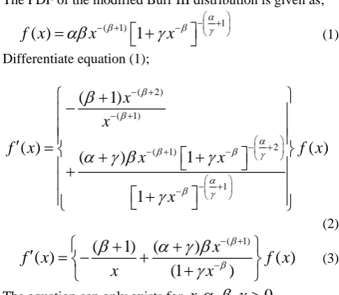
The PDF of the modified Burr III distribution is given as;
1 ( 1)
( )
1
f x
x
x
(1)
Differentiate equation (1);
( 2) ( 1)
2 ( 1)
1
(
1)
( )
( )
(
)
1
1
x
x
f x
f x
x
x
x
(2)
( 1)
(
1)
(
)
( )
( )
(1
)
x
f x
f x
x
x
(3)
The equation can only exists for
x
, , ,
0.
The first order ODE for the PDF of modified Burr III
distribution can be obtained from any given values of
, , .
Some examples are given in Table 1.
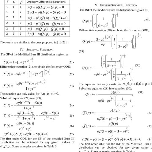
Table 1: ODE for the PDF for some given values of the
parameters
Ordinary Differential Equations
1
1
1
(
x
1)
f x
( ) 2 ( )
f x
0
1
1
2
x x
(
1)
f x
( ) (2
x
1) ( )
f x
0
1
2
1
x x
(
2)
f x
( ) (2
x
1) ( )
f x
0
1
2
2
(
x
2)
f x
( )
2 ( )
f x
0
2
1
1
2 2(
1)
( ) (3
1) ( )
0
x x
f x
x
f x
2
1
2
2 2(
1)
( ) 3(
1) ( )
0
x x
f x
x
f x
2
2
1
2 2(
1)
( ) 3(
1) ( )
0
x x
f x
x
f x
2
2
2
2 2(
1)
( ) (3
5) ( )
0
x x
f x
x
f x
Modified Burr III Distribution: Ordinary
Differential Equations
Hilary I. Okagbue,
Member,
IAENG
, Pelumi E. Oguntunde, Abiodun A. Opanuga
and Patience I. Adamu
[image:1.595.303.546.281.492.2]Differentiate equation (3);
2 ( 1) 2
2 2
( 2)
( 1)
(
1)
(
)
(
)
(1
)
( )
( )
(
1)(
)
(1
)
(
1)
(
)
+
( )
(1
)
x
x
x
f
x
f x
x
x
x
f x
x
x
(4)
The equation can only exists for
x
, , ,
0
.
The presented equations acquired from equation (3) are
required in the further breaking down of equation (4);
( 1)
(
1)
(
)
( )
(1
)
( )
x
f x
x
x
f x
(5)
( 1)
(
)
( )
(
1)
(1
)
( )
x
f x
x
f x
x
(6)
2 2
( 1)
(
)
( )
1
1
( )
x
f x
x
f x
x
(7)
2 2 ( 1) 2
2
(
)
(
)
( )
1
(1
)
( )
x
f x
x
f x
x
(8)
( 1)
(
) (
1)
( )
(
1)
1
(1
)
( )
x
f x
x
f x
x
(9)
( 2)
(
) (
1)
1
( )
(
1)
(1
)
( )
x
f x
x
x
f x
x
(10)
Substitute equations (5), (8) and (10) into equation (4);
2
2
2
( )
1
( )
( )
1
( )
1
( )
( )
( )
( )
1
f x
f x
x
f
x
f x
f
x
f x
f x
x
f x
x
x
(11)
1
(1)
(1
)
f
(12)
1
2
(
)
(
1)(1
)
(1)
(1
)
1
((
)
(
1)(1
))
(1
)
f
(13)
The ODE can be obtained for
, , .
The results are similar to the ones proposed in [10-23].
III.
QUANTILE FUNCTION
The QF of the Modified Burr III distribution is given as;
1
1
1
( )
1
Q p
p
(14)
Differentiate equation (14), to obtain the first order ODE;
1 1 1
1
1
( )
p
1
Q p
p
(15)
1
1
1
1
1
( )
1
1
1
p
Q p
p
p
(16)
The equation can only exists for
, ,
0, 0
p
1.
Substitute equation (14);
1
( )
( )
1
1
Q p
Q p
p
p
(17)
1
( )
( )
(
)
Q p
Q p
p
p
(18)
( )
( )
(1
)
Q p
Q p
p
p
(19)
(1
)
( )
( )
0
p
p
Q p
Q p
(20)
The first order ODE for the QF of the modified Burr III
distribution can be acquired for the particular values of
, , .
Table 2: ODE for the QF for some selected values
Ordinary Differential Equations
1
1
1
p
(1
p Q p
)
( )
Q p
( )
0
1
1
2
2 (1
p
p Q p
)
( )
Q p
( )
0
2
1
1
2(1
)
( ) 2 ( )
0
p
p Q p
Q p
2
1
2
2(1
)
( )
( )
0
p
p Q p
Q p
2
2
1
p
(1
p Q p
)
( )
Q p
( )
0
2
2
2
2 (1
p
p Q p
)
( )
Q p
( )
0
The results are similar to the ones proposed in [10-23].
IV.
SURVIVAL FUNCTION
The SF of the Modified Burr III distribution is given as;
( ) 1 [1
]
S t
t
(21)
Differentiate equation (21), to obtain the first order ODE;
1 ( 1)
( )
1
S t
t
t
(22)
( 1)
(1
)
( )
1
t
t
S t
t
(23)
The equation can only exists for
t
, , ,
0.
Substitute equation (21) into (23);
( 1)
(1
( ))
( )
1
t
S t
S t
t
(24)
1 1
(1
( ))
(1
( ))
( )
(1
)
S t
S t
S t
t
t
t
t
(25)
(1
( ))
( )
(
)
S t
S t
t t
(26)
(
) ( )
(1
( ))
0
t t
S t
S t
(27)
The first order ODE for the SF of the modified Burr III
distribution can be obtained for any given values of
, , .
Some examples are given in Table 3.
Table 3: ODE for the SF for some selected values
Ordinary Differential Equations
1
1
1
t t
(
1) ( )
S t
S t
( ) 1
0
1
1
2
t t
(
1) ( ) 2 ( )
S t
S t
2
0
1
2
1
t t
(
2) ( )
S t
S t
( ) 1
0
1
2
2
t t
(
2) ( ) 2 ( ) 1
S t
S t
0
2
1
1
2(
1) ( ) 2 ( ) 2
0
t t
S t
S t
2
1
2
2(
1) ( ) 4 ( ) 4
0
t t
S t
S t
2
2
1
2(
2) ( ) 2 ( ) 2
0
t t
S t
S t
2
2
2
2(
2) ( ) 4 ( ) 4
0
t t
S t
S t
The results are similar to the ones proposed in [10-23].
V.
INVERSE SURVIVAL FUNCTION
The ISFof the modified Burr III distribution is given as;
1
1
1
( )
1
(1
)
Q p
p
(28)
Differentiate equation (28) to obtain the first order ODE;
1 1 1
(1
)
1
1
( )
1
(1
)
p
Q p
p
(29)
1
1
1
1
1
(1
)
( )
1
1
(1
)
1
(1
)
p
Q p
p
p
(30)
The equation can only exists for
, ,
0, 0
p
1.
Substitute equation (28) into equation (30);
1
( )
( )
1
(1
)
1
(1
)
Q p
Q p
p
p
(31)
1
( )
( )
((1
) (1
)
)
Q p
Q p
p
p
(32)
( )
( )
(1
)(1 (1
) )
Q p
Q p
p
p
(33)
(1
p
)(1 (1
p
) )
Q p
( )
Q p
( )
0
(34)
The first order ODE for the ISF of the Modified Burr III
distribution can be obtained for any given values of
, , .
[image:3.595.296.535.80.566.2]
Some examples are given in Table 4.
Table 4: ODE for the ISF for some selected values
Ordinary Differential Equations
1 1
1
p
(1
p Q p
)
( )
Q p
( )
0
1 1
2
2 (1
p
p Q p
)
( )
Q p
( )
0
1 2
1
2(1
p
)(1
p Q p
)
( )
Q p
( )
0
1 2
2
4(1
p
)(1
p Q p
)
( )
Q p
( )
0
2 1
1
2(1
p
)(1 (1
p
) )
Q p
( ) 2 ( )
Q p
0
2 1
2
2(1
p
)(1 (1
p
) )
Q p
( )
Q p
( )
0
2 2
1
p
(1
p Q p
)
( )
Q p
( )
0
The results are similar to the ones proposed in [10-23].
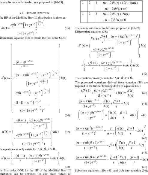
VI.
HAZARD FUNCTION
The HF of the Modified Burr III distribution is given as;
1 ( 1)
1
( )
1 [1
]
t
t
h t
t
(35)
Differentiate equation (35) to obtain the first order ODE;
( 2) ( 1) 2 ( 1) 1 1 ( 1) 2 1
(
1)
(
)
1
( )
( )
1
1
(1 [1
]
)
(1 [1
]
)
t
t
t
t
h t
h t
t
t
t
t
t
(36)
( 1) 1 ( 1)
(
1)
(
)
1
( )
( )
1
(1 [1
]
)
t
t
t
h t
h t
t
t
t
(37)
The equation can only exists for
t
, , ,
0.
( 1)
(
1)
(
)
( )
( )
( )
1
t
h t
h t
h t
t
t
(38)
The first order ODE for the HF of the Modified Burr III
distribution can be obtained for any given values of
, , .
[image:4.595.54.549.49.633.2]
Some examples are given in Table 5.
Table 5: ODE for the HF for some selected values
Ordinary Differential Equations
1
1
1
2
(
1) ( ) 2 ( )
(
1)
( )
0
t
h t
h t
t
h t
1
1
2
2
(
1) ( ) (2
1) ( )
(
1)
( )
0
t t
h t
t
h t
t t
h t
1
2
1
2
(
2) ( ) (2
1) ( )
(
2)
( )
0
t t
h t
t
h t
t t
h t
1
2
2
2
(
2) ( ) 2 ( )
(
2)
( )
0
t t
h t
h t
t
h t
The results are similar to the ones proposed in [10-23].
Differentiate equation (38);
2 ( 1) 2 2 2
( 2)
( 1)
1
(
)
(
)
( )
1
( )
( )
(
)
1
(
1)
(
)
+
( )
( )
1
t
h t
t
t
h t
h t
t
t
t
h t
h t
t
t
(39)
The equation can only exists for
t
, , ,
0.
The presented equations derived from equation (38) are
required in the further breaking down of equation (39);
( 1)
(
1)
(
)
( )
( )
(1
)
( )
t
h t
h t
t
t
h t
(40)
( 1)
(
)
( )
1
( )
(1
)
( )
t
h t
h t
t
h t
t
(41)
2 2
( 1)
(
)
( )
1
( )
1
( )
t
h t
h t
t
h t
t
(42)
2 2 ( 1) 2
2
(
)
(
)
( )
1
( )
(1
)
( )
t
h t
h t
t
h t
t
(43)
( 1)(
) (
1)
( )
1
1
( )
(1
)
( )
t
h t
h t
t
h t
t
(44)
( 2)(
) (
1)
1
( )
(
1)
( )
(1
)
( )
t
h t
h t
t
t
h t
t
(45)
Substitute equations (40), (43) and (45) into equation (39);
2 2
1
( )
( )
( )
( )
( )
( )
1
( )
( )
h t
t
h t
h t
h t
h t
h t
h t
h t
t
1
( )
(
1)
( )
( )
( )
h t
h t
h t
t
h t
t
11
(1)
1 [1
]
h
(47)
(
1)
(
)
(1)
(1)
(1)
1
h
h
h
t
(48)
The ODEs can be obtained for any given values of
, , .
VII.
REVERSED HAZARD FUNCTION
The RHF of the modified Burr III distribution is given as;
( 1)
( )
1
t
j t
t
(49)
Differentiate equation (49), to obtain the first order ODE;
( 2) ( 1) 2
( 1) 1
(
1)
(1
)
( )
( )
(1
)
t
t
t
j t
j t
t
t
(50)
( 1)
(
1)
( )
( )
(1
)
t
j t
j t
t
t
(51)
The equation can only exists for
t
, , ,
0.
(
1)
( )
( )
j t
( )
j t
j t
t
(52)
The first order ODE for the RHFof the modified Burr III
distribution is given by;
2
( )
(
1) ( )
( )
0
tj t
j t
tj t
(53)
(1)
1
j
(54)
The results are similar to the ones proposed in [10-23].
VIII.
CONCLUDING REMARKS
Ordinary differential equations (ODEs) have been obtained
for the probability functions of modified Burr III
distribution. This differential calculus and efficient algebraic
simplifications were used to derive the various classes of the
ODEs. The parameter and the supports that characterize the
distribution determine the nature, existence, orientation and
uniqueness of the ODEs. The results are in agreement with
those available in scientific literature. Furthermore several
methods can be used to obtain desirable solutions to the
ODEs.[25-40]. This method of characterizing distributions
cannot be applied to distributions whose PDF or CDF are
either not differentiable or the domain of the support of the
distribution contains singular points.
ACKNOWLEDGMENT
The comments of the reviewers were very helpful and led
from sponsorship from the Statistics sub-cluster of the
Industrial Mathematics Research Group
(TIMREG) of
Covenant University and
Centre for Research, Innovation
and Discovery
(CUCRID), Covenant University, Ota,
Nigeria.
REFERENCES
[1] G. Derflinger, W. Hörmann and J. Leydold, “Random variate generation by numerical inversion when only the density is known,”
ACM Transac.Model. Comp. Simul., vol. 20, no. 4, Article 18, 2010.
[2] G. Steinbrecher and W.T. Shaw, “Quantile mechanics” Euro. J. Appl. Math., vol. 19, no. 2, pp. 87-112, 2008.
[3] H.I. Okagbue, M.O. Adamu and T.A. Anake “Quantile Approximation of the Chi-square Distribution using the Quantile Mechanics,” In Lecture Notes in Engineering and Computer Science: Proceedings of The World Congress on Engineering and Computer Science 2017, 25-27 October, 2017, San Francisco, U.S.A., pp 477-483.
[4] H.I. Okagbue, M.O. Adamu and T.A. Anake “Solutions of Chi-square Quantile Differential Equation,” In Lecture Notes in Engineering and Computer Science: Proceedings of The World Congress on Engineering and Computer Science 2017, 25-27 October, 2017, San Francisco, U.S.A., pp 813-818.
[5] W.P. Elderton, Frequency curves and correlation, Charles and Edwin Layton. London, 1906.
[6] N. Balakrishnan and C.D. Lai, Continuous bivariate distributions, 2nd edition, Springer New York, London, 2009.
[7] N.L. Johnson, S. Kotz and N. Balakrishnan, Continuous Univariate Distributions, Volume 2. 2nd edition, Wiley, 1995.
[8] N.L. Johnson, S. Kotz and N. Balakrishnan, Continuous univariate distributions, Wiley New York. ISBN: 0-471-58495-9, 1994. [9] H. Rinne, Location scale distributions, linear estimation and
probability plotting using MATLAB, 2010.
[10] H.I. Okagbue, P.E. Oguntunde, A.A. Opanuga, E.A. Owoloko “Classes of Ordinary Differential Equations Obtained for the Probability Functions of Fréchet Distribution,” In Lecture Notes in Engineering and Computer Science: Proceedings of The World Congress on Engineering and Computer Science 2017, 25-27 October, 2017, San Francisco, U.S.A., pp 186-191.
[11] H.I. Okagbue, P.E. Oguntunde, P.O. Ugwoke, A.A. Opanuga “Classes of Ordinary Differential Equations Obtained for the Probability Functions of Exponentiated Generalized Exponential Distribution,” In Lecture Notes in Engineering and Computer Science: Proceedings of The World Congress on Engineering and Computer Science 2017, 25-27 October, 2017, San Francisco, U.S.A., pp 192-197.
[12] H.I. Okagbue, A.A. Opanuga, E.A. Owoloko, M.O. Adamu “Classes of Ordinary Differential Equations Obtained for the Probability Functions of Cauchy, Standard Cauchy and Log-Cauchy Distributions,” In Lecture Notes in Engineering and Computer Science: Proceedings of The World Congress on Engineering and Computer Science 2017, 25-27 October, 2017, San Francisco, U.S.A., pp 198-204.
[13] H.I. Okagbue, S.A. Bishop, A.A. Opanuga, M.O. Adamu “Classes of Ordinary Differential Equations Obtained for the Probability Functions of Burr XII and Pareto Distributions,” In Lecture Notes in Engineering and Computer Science: Proceedings of The World Congress on Engineering and Computer Science 2017, 25-27 October, 2017, San Francisco, U.S.A., pp 399-404.
[14] H.I. Okagbue, M.O. Adamu, E.A. Owoloko and A.A. Opanuga “Classes of Ordinary Differential Equations Obtained for the Probability Functions of Gompertz and Gamma Gompertz Distributions,” In Lecture Notes in Engineering and Computer Science: Proceedings of The World Congress on Engineering and Computer Science 2017, 25-27 October, 2017, San Francisco, U.S.A., pp 405-411.
[15] H.I. Okagbue, M.O. Adamu, A.A. Opanuga and J.G. Oghonyon “Classes of Ordinary Differential Equations Obtained for the Probability Functions of 3-Parameter Weibull Distribution,” In Lecture Notes in Engineering and Computer Science: Proceedings of The World Congress on Engineering and Computer Science 2017, 25-27 October, 2017, San Francisco, U.S.A., pp 539-545.
The World Congress on Engineering and Computer Science 2017, 25-27 October, 2017, San Francisco, U.S.A., pp 546-551.
[17] H.I. Okagbue, M.O. Adamu, E.A. Owoloko and S.A. Bishop “Classes of Ordinary Differential Equations Obtained for the Probability Functions of Half-Cauchy and Power Cauchy Distributions,” In Lecture Notes in Engineering and Computer Science: Proceedings of The World Congress on Engineering and Computer Science 2017, 25-27 October, 2017, San Francisco, U.S.A., pp 552-558.
[18] H.I. Okagbue, P.E. Oguntunde, A.A. Opanuga and E.A. Owoloko “Classes of Ordinary Differential Equations Obtained for the Probability Functions of Exponential and Truncated Exponential Distributions,” In Lecture Notes in Engineering and Computer Science: Proceedings of The World Congress on Engineering and Computer Science 2017, 25-27 October, 2017, San Francisco, U.S.A., pp 858-864.
[19] H.I. Okagbue, O.O. Agboola, P.O. Ugwoke and A.A. Opanuga “Classes of Ordinary Differential Equations Obtained for the Probability Functions of Exponentiated Pareto Distribution,” In Lecture Notes in Engineering and Computer Science: Proceedings of The World Congress on Engineering and Computer Science 2017, 25-27 October, 2017, San Francisco, U.S.A., pp 865-870.
[20] H.I. Okagbue, O.O. Agboola, A.A. Opanuga and J.G. Oghonyon “Classes of Ordinary Differential Equations Obtained for the Probability Functions of Gumbel Distribution,” In Lecture Notes in Engineering and Computer Science: Proceedings of The World Congress on Engineering and Computer Science 2017, 25-27 October, 2017, San Francisco, U.S.A., pp 871-875.
[21] H.I. Okagbue, O.A. Odetunmibi, A.A. Opanuga and P.E. Oguntunde “Classes of Ordinary Differential Equations Obtained for the Probability Functions of Half-Normal Distribution,” In Lecture Notes in Engineering and Computer Science: Proceedings of The World Congress on Engineering and Computer Science 2017, 25-27 October, 2017, San Francisco, U.S.A., pp 876-882.
[22] H.I. Okagbue, M.O. Adamu, E.A. Owoloko and E.A. Suleiman “Classes of Ordinary Differential Equations Obtained for the Probability Functions of Harris Extended Exponential
Distribution,” In Lecture Notes in Engineering and Computer Science: Proceedings of The World Congress on Engineering and Computer Science 2017, 25-27 October, 2017, San Francisco, U.S.A., pp 883-888.
[23] H.I. Okagbue, M.O. Adamu, T.A. Anake Ordinary Differential Equations of the Probability Functions of Weibull Distribution and their application in Ecology, Int. J. Engine. Future Tech., vol. 15, no. 4, pp. 57-78, 2018.
[24] A. Ali, S.A. Hasnain and M. Ahmad, “Modified burr III distribution, properties and applications” Pak. J. Stat., vol. 31, no. 6, pp. 697-708, 20
[25] A. A. Opanuga, H. I. Okagbue, E. A. Owoloko and O. O. Agboola, Modified Adomian Decomposition Method for Thirteenth Order Boundary Value Problems, Gazi Uni. J. Sci., vol. 30, no. 4, pp. 454-461, 2017.
[26] A.A. Opanuga, H.I. Okagbue and O.O. Agboola “Application of Semi-Analytical Technique for Solving Thirteenth Order Boundary Value Problem,” Lecture Notes in Engineering and Computer Science: Proceedings of The World Congress on Engineering and Computer Science 2017, 25-27 October, 2017, San Francisco, U.S.A., pp 145-148.
[27] A.A. Opanuga, H.I. Okagbue, O.O. Agboola, "Irreversibility Analysis of a Radiative MHD Poiseuille Flow through Porous Medium with Slip Condition," Lecture Notes in Engineering and Computer Science: Proceedings of The World Congress on Engineering 2017, 5-7 July, 2017, London, U.K., pp. 167-171.
[28] A.A. Opanuga, E.A. Owoloko, H.I. Okagbue, “Comparison Homotopy Perturbation and Adomian Decomposition Techniques for Parabolic Equations,” Lecture Notes in Engineering and Computer Science: Proceedings of The World Congress on Engineering 2017, 5-7 July, 2015-7, London, U.K., pp. 24-25-7.
[29] A.A. Opanuga, E.A. Owoloko, H. I. Okagbue, O.O. Agboola, "Finite Difference Method and Laplace Transform for Boundary Value Problems," Lecture Notes in Engineering and Computer Science: Proceedings of The World Congress on Engineering 2017, 5-7 July, 2017, London, U.K., pp. 65-69.
[30] A.A. Opanuga, E.A. Owoloko, O.O. Agboola, H.I. Okagbue, "Application of Homotopy Perturbation and Modified Adomian Decomposition Methods for Higher Order Boundary Value Problems," Lecture Notes in Engineering and Computer Science: Proceedings of The World Congress on Engineering 2017, 5-7 July, 2017, London, U.K., pp. 130-134.
[31] A.A. Opanuga, S.O. Edeki, H.I. Okagbue, G.O. Akinlabi, A.S. Osheku and B. Ajayi, “On numerical solutions of systems of ordinary differential equations by numerical-analytical method”, Appl. Math. Sciences, vol. 8, no. 164, pp. 8199 – 8207, 2014.
[32] S.O. Edeki , A.A. Opanuga, H.I. Okagbue , G.O. Akinlabi, S.A. Adeosun and A.S. Osheku, “A Numerical-computational technique for solving transformed Cauchy-Euler equidimensional equations of homogenous type. Adv. Studies Theo. Physics, vol. 9, no. 2, pp. 85 – 92, 2015.
[33] S.O. Edeki , E.A. Owoloko , A.S. Osheku , A.A. Opanuga , H.I. Okagbue and G.O. Akinlabi, “Numerical solutions of nonlinear biochemical model using a hybrid numerical-analytical technique”,
Int. J. Math. Analysis, vol. 9, no. 8, pp. 403-416, 2015.
[34] A.A. Opanuga , S.O. Edeki , H.I. Okagbue and G.O. Akinlabi, “Numerical solution of two-point boundary value problems via differential transform method”, Global J. Pure Appl. Math., vol. 11, no. 2, pp. 801-806, 2015.
[35] A.A. Opanuga, S.O. Edeki, H.I. Okagbue and G. O. Akinlabi, “A novel approach for solving quadratic Riccati differential equations”,
Int. J. Appl. Engine. Res., vol. 10, no. 11, pp. 29121-29126, 2015. [36] A.A Opanuga, O.O. Agboola and H.I. Okagbue, “Approximate
solution of multipoint boundary value problems”, J. Engine. Appl. Sci., vol. 10, no. 4, pp. 85-89, 2015.
[37] A.A. Opanuga, O.O. Agboola, H.I. Okagbue and J.G. Oghonyon, “Solution of differential equations by three semi-analytical techniques”, Int. J. Appl. Engine. Res., vol. 10, no. 18, pp. 39168-39174, 2015.
[38] A.A. Opanuga, S.O. Edeki, H.I. Okagbue, S.A. Adeosun and M.E. Adeosun, “Some Methods of Numerical Solutions of Singular System of Transistor Circuits”, J. Comp. Theo. Nanosci., vol. 12, no. 10, pp. 3285-3289, 2015.
[39] S.O. Edeki, H.I. Okagbue , A.A. Opanuga and S.A. Adeosun, “A semi - analytical method for solutions of a certain class of second order ordinary differential equations”, Applied Mathematics, vol. 5, no. 13, pp. 2034 – 2041, 2014.
[40] S.O. Edeki, A.A Opanuga and H.I Okagbue, “On iterative techniques for numerical solutions of linear and nonlinear differential equations”,
J. Math. Computational Sci., vol. 4, no. 4, pp. 716-727, 2014.