!"$#&%'()* ,+"#-%
./##&!01 2034'5'5#- %#&.6!01*
798;:=<?>@BAC>9DFE(AHG
I8KJ@L89MN@LOQPECRSUTWVXY:[Z@
V]\C@CO^@H_M`@H:YXba
Abstract The problems of Boolean satisfiability (SAT) and automatic test pattern
gen-eration (ATPG) are strongly related - both in terms of application areas
(pre-manufacturing design validation and post-(pre-manufacturing testing), as well as in terms of techniques used in their practical solutions (searching large combina-torial spaces through efficient pruning). However, historically these domains have evolved somewhat independently with limited interaction. While ATPG has been primarily driven by reasoning based on circuit structure, SAT has fo-cussed on reasoning using conjunctive normal form (CNF) representations of Boolean formulas. In this chapter, we introduce these problems, describe key techniques used to solve them in practice, and highlight the common themes and differences between them.
cdfe^c gihjlk`monqprsjgtmoh
The problems of Boolean satisfiability (SAT) and automatic test pattern generation (ATPG) have been investigated intensively for many decades. Bool-ean satisfiability serves as an important reference problem in complexity theory of Computer Science. It has been shown that many difficult decision problems from various application domains can be reduced to the Boolean satisfiabil-ity problem. Algorithms for solving this problem have been an active field of research and steady progress has been achieved over many years.
SAT and ATPG algorithms have received even stronger interest more re-cently, since they have been used successfully as Boolean engines for equiv-alence checking (see Chapter 13) and logic synthesis (see Chapter 2). In this chapter, we ignore the physical aspects of testing and do not consider testing of sequential circuits. Our interest is exclusively in the combinatorial search problems in SAT and ATPG.
Traditionally, the research domains of SAT and ATPG developed quite inde-pendently of each other. With a broad spectrum of applications as background, the research in SAT typically focused on general concepts useful in diverse fields. Due to the more specialized problem formulation, research in ATPG focused on techniques that are fine-tuned to dealing with digital circuits. In general, however, there are a lot of commonalities between the notions and methods developed in the two research domains. This chapter describes the basic concepts of SAT and combinational ATPG. Where possible, it attempts to bridge the gap between the terminology commonly used in the two areas.
cdfed j 1hn jl k`mNF mNk1p FjgtmNh9
Algorithms for automatic test pattern generation in combinational circuits are traditionally based on a gate netlist description of the circuit under test (CUT). SAT algorithms typically represent the circuit by a conjunctive normal form (CNF) formula. This distinction is not very sharp, however. SAT and ATPG are closely related problems and there also exist various ATPG tools based on a CNF representation of the circuit. Note that a gate netlist description can always be translated into a CNF formula, as described in the next section, but not vice versa. In the following, we present the problem formulations for Boolean satisfiability and combinational stuck-at fault testing based on the conventional CNF- and gate netlist representations, respectively.
¡B¢£¢£¡ ¤ ¥¦"§¨s¦`¤ª©ª«U¬®¦`¥¯°²±l³²´µ¥¯° ±¦"¶
·
±©ª«
·
´«¸±¹ «¸³º«¸©¼»
Instances of SAT are most often represented as CNF formulas. A CNF for-mula is a conjunction (product) of clauses, where a clause is a disjunction (sum) of literals, and a literal is either a variable or its complement. For exam-ple½¾¿ÁÀÂBÃ"ÄÀCÅÇÆU¿ÄÀ;ÂKÃ"ÀÈUÆ , denotes a CNF formula with two clauses and
three variables.
The Boolean satisfiability problem for a CNF formula is formulated as fol-lows: Given a CNF formula,½ , representing a Boolean function,É¿ÀÂÇÊUËÌËUË?ÊÀÍÆ ,
the satisfiability problem consists of identifying a set of assignments to the for-mula variables, ÎÏÀ;Âо2ÑÒÂÇÊUËUËÌË?ÊWÀt;2ÑUÍLÓ , such that all clauses are satisfied,
Combinational circuits can easily be represented using CNF formulas. A CNF formula is associated with each gate, and captures the consistent assign-ments between the gate inputs and output. The CNF formula for the circuit is the conjunction of the CNF formulas for the gates in the circuit; assignments to the circuit nodes are consistent if and only if the assignments are consistent for the inputs and output of each gate in the circuit.
The derivation of the CNF formula for a gateÀÚ¾ É¿ÛÜÂÝÊÌËUËUË^ÊÛ]ÞWÆ is
straight-forward. First, a new Boolean functionßUྠÀá"É¿ÛÜÂÝÊÌËUËUËâÊWÛ]ÞWÆ is defined.
Observe thatßUà only assumes value 1 providedÀ andÉ¿ÁÛºÂÝÊÌËUËÌË?ÊWÛ]ÞWÆ assume
the same value. Next,ßUà is represented as a product-of-sums form,½5à . Hence,
the CNF formula½ à assumes value 1 if and only if the value of À is equal to
the value of É¿ÛºÂUÊÌËUËÌËãÊÛ]ÞWÆ . As an example consider a 2-input AND gate, À²¾ äåHæ . The resulting formula becomes ßUàC¿À(ÊWäLÊWæÇƾ Àá`É¿ÁäCÊæÇÆs¾ Àå¿ äçà æÆBà ÀèåÝäFåÇæ}¾¿ ÀéÃNäiÆ5å¿ÀÃ"æÇÆêåë¿ÁÀà äºÃ æÇƾ ½5à .
¡B¢£¢£¢ ìs±©ª¦"©ª³º«
·
©í±¦"¶
·
©ª¨"¤ªîïݱè©ð´± ¨³K© ©ª
·
©ª«¸¦`ì
Techniques of test generation most often rely on a gate netlist description of the circuit. A gate netlist can be modeled as a Boolean network. A Boolean network is a graph, with vertices (referred also to as nodes, variables or signals) representing gates and directed edges representing connections between gates. Each vertex has a function associated with it which corresponds to the function of the gate it represents.
In the following, we always assume that each function in the Boolean net-work is very simple such that it can be implemented by one of the primitive gate types AND, OR, NOT, NAND or NOR. Each of these gates can have an arbitrary number of inputs. Extending the ATPG techniques of this chapter to XOR, XNOR or other more complex functions is possible but will not be further considered.
The goal of testing is to detect physical defects on a chip inflicted by the fabrication process or those occurring later during the operation of the chip. Physical defects are described at the gate level by certain fault models. The single stuck-at fault is a widely accepted model. It assumes that a single line in the combinational circuit fails to change its logic value and is “stuck” at a constant value of 0 or 1.
òó ôöõ
÷ø ù
úüûýöþöÿû
Circuit under test (CUT).
starting point of all operations is a list of faults that must be detected by the tests to be determined. The faults in the fault list are targeted one after the other and for every fault a test is derived by the ATPG algorithm. In this chapter, we exclusively consider deterministic ATPG. For reasons of simplicity the word “deterministic” is often omitted.
The problem of test generation for single stuck-at faults in combinational circuits is illustrated in Figure 12.1. For a given gate netlist there is a fault list
¾Î (ÂUÊ!ÅÌÊUËUËÌË?Ê!#"ÌÓ containing all faults for which a test has to be generated.
These faults are called target faults. Let have $ primary input signals and
%
primary output signals and let y¾¿&Ò¾ ÑÒÂUÊ!&¸Å}¾ ѸÅUÊÌËUËUËâÊ!&(' ¾ Ñ(' Æ be the
response of the fault-free circuit and z¾¿&ÒÂf¾ Ñ*)
Â
Ê!&¸Å}¾ Ñ+)
Å
ÊUËUËÌË?Ê!&('N¾ Ñ*)
'
Æ be
the response of the faulty circuit to some input stimulus x ¾/¿ÁÀ ¾9ÛºÂÇÊWÀLÅ ¾ Û Å ÊÌËUËÌË?ÊWÀ Í ¾/Û Í Æ withÑ-,?ÊÑ )
Þ
ÊÛ "/. Î 0ÊÌÔ¸Ó . The input stimulus x is called a
test for a fault if and only if the circuit response z in the presence of is
different from the response y of the fault-free circuit. There may not exist a test for every fault in a circuit. Untestable faults are also called redundant. The task of a deterministic ATPG algorithm is to calculate a test x for a given fault
if a test exists, or to prove its untestability otherwise. An input stimulus x
that detects a fault is also called a test vector or test pattern for fault . cdfe1 r"mN sgihjgtmNh1$n jk1gihgtjgr
jl
After introducing the basic problem formulations for SAT and ATPG we now consider the algorithms for solving these problems. The basic SAT pro-cedure will be described in Section 12.4. This section gives an introduction to the general combinational ATPG procedure. It will become apparent how ATPG and SAT are generally related.
¡B¢£2]£¡ ³µ¥ìs«Ò¤ ±³4365"±l¹ ©
·
A combinational circuit with $ primary inputs and
%
primary outputs is specified at the gate level by an%
-ary function É87:9 Í<;
9
'
, where 9 is
alpha-AND 0 1 X D >
0 0 0 0 0 0
1 0 1 X D >
X 0 X X X X
D 0 D X D 0
> 0 > X 0 >
OR 0 1 X D >
0 0 1 X D >
1 1 1 1 1 1
X X 1 X X X
D D 1 X D 1
> > 1 X 1 >
? @
0 1
1 0
X X
D > > A B CDEF:GH
AND-, OR-, NOT-operation in the 5-valued logic alphabetIKJ .
bets are required. In order to describe the faulty behavior of a circuit, Roth’s D-calculus [37] has become widely accepted. In Roth’s notation a signal is assigned the logic valueL if it assumes 1 in the fault-free and 0 in the faulty
circuit. In the opposite case, if the signal is 0 in the fault-free and 1 in the faulty circuit, it is denoted byM . For logic values being equal in the fault-free
and faulty cases, namely 0 or 1, the signal value is denoted 0 or 1, respectively. With these notations we obtain the logic alphabet94N¾6Î 0ÊÌÔwÊGMÊ MºÓ . For test
generation it is of advantage to introduce a fifth logic value, X, describing the case where no unique logic value has been assigned. This value is usually re-ferred to as the don’t care or unknown value. Including X into 94N results in
the five-valued logic alphabet9POº¾6Î 0ÊUÔÒÊGQÊGMFÊ M Ó . A 5-valued algebra over 9 O can be obtained by straightforward extensions of the usual operations of
conjunction, disjunction, and negation for9Å ; the truth tables for these
exten-sions are shown in Table 12.1. Although some applications especially in delay testing require more sophisticated logic alphabets [2, 14] Roth’s D-alphabet, to this date, forms the basis for many modern ATPG algorithms.
¡B¢£2]£¢ ±©/3 ì ±³µì"¥¯«¸©/5"° ·SR
±¦ ¥Ú¬¯é¬s«¸UT
It is the great merit of Roth’s D-calculus that it allows us to completely de-scribe the faulty behavior of the circuit on its structural gate-level description paving the way for efficient heuristics. In this section, we describe a conven-tional procedure of test generation based on the D-alphabet operating on a gate netlist representation of the circuit.
For illustration of the general ATPG procedure consider the circuit of Fig-ure 12.2. Consider the single stuck-at-1 (s-a-1) fault at signalV . Obviously, an
input vector can only be a test for this fault if it exhibits a faulty logic value or fault signal at the fault lineV . This process is called fault excitation, fault
setup or fault injection. In our example, signalV has to be controlled from the
primary inputs in such a way that it assumes a logic 0 in the fault-free case. If signalV is 0 in the fault-free case and 1 in the faulty case, then it assumes the
XZY X[ X\ X] X^ X_ Xa` Xb Xc XYd XYeY XY[ XY\
f
Y
f
[
gehijhk
lmonap qFrs
t
rZs
uwvxyjz {|}~y vxyjz{|}~y
a
!GF
Fault injection.
The problem of identifying a set of value assignments at the primary inputs such that a faulty logic value is produced at the fault line is called the controlla-bility problem in ATPG. Further, it must be ensured that a faulty signal at fault lineÉ can propagate to at least one primary output of the circuit. Identifying
a set of value assignments at the primary inputs such that a signal change atÉ
from 0 to 1 or from 1 to 0 can propagate to at least one primary output is called the observability problem forÉ . Test generation for stuck-at faults requires the
simultaneous solution of the controllability and the observability problem for a given fault lineÉ .
After fault injection all common test generators perform logic implications, i.e., they make value assignments that can be derived from fault injection. In our example, we assume that the implication procedure produces the new value assignmentsè¾0 ,¾0 ,Vw¾ M andVÏÅç¾ M as shown in Figure 12.2. This
is the starting point for all subsequent steps. Among the signal assignments generated during the ATPG process, there are two sets of signals that are of particular interest, called the D-frontier and the J-frontier.
The D-frontier consists of all fault signals, i.e., signals being assigned
either D or M , which are input signals of logic gates whose output signal is
unspecified. The D-frontier indicates how far the faulty signals have propa-gated from the fault location towards the primary outputs. In Figure 12.2 fault injection has produced the D-frontier¾ÎVwÂÇÊZV¸ÅÓ .
The J-frontier consists of all output signals of gates being assigned a value
not completely justified by the value assignments at the gate inputs. In Figure 12.2 two unjustified lines9¾9Î âÊÓ have been created. For a valid test, they
have to be justified in subsequent steps of test generation.
Using these notations the task of a test generator can be reformulated as follows: find a set of binary value assignments at the primary inputs of the circuit, such that
the D-frontier reaches the primary outputs, i.e., at least one primary out-put assumes a faulty value (solve the observability problem),
the J-frontier reaches the primary inputs, i.e., there exist no unjustified lines in the interior of the circuit (solve the controllability problem).
Note that the controllability problem is essentially a SAT problem, and is solved by identifying a set of assignments for the inputs of the circuit such that all signals of the J-frontier are satisfied. Therefore, not surprisingly, many algorithmic concepts for combinational test generation are closely related to those of SAT solving methods and SAT solvers can be used to solve the ATPG problem in parts or entirely.
To accomplish the above two tasks most algorithms for deterministic test generation proceed step by step, assigning appropriate logic values at well-selected signals in the circuit such that the D-frontier is moved towards the primary outputs and the J-frontier is moved towards the primary inputs.
Along the process of test generation we distinguish two types of value as-signments. First, we consider necessary asas-signments. Necessary assignments are uniquely determined by the current situation of value assignments in the circuit and any test vector that can be generated starting from the current sit-uation must contain this value assignment. In Figure 12.2 fault injection has produced the necessary value assignments5¾0 ,о0 ,VÒÂf¾ M ,V¸Å¾ M .
Be-sides necessary assignments every test generator makes optional assignments. Optional assignments are assignments that can be made in order to reach the goal of generating a test vector. The existence of optional assignments results from the fact that there usually exists more than just one test vector for a given fault. By making optional assignments we continue to restrict the number of possible test vectors until we finally end up with exactly one. The choice of optional value assignments is subject to heuristics.
Test generation can be understood as a sequence of making optional and necessary assignments. Figure 12.3 shows a general procedure that outlines the steps for combinational test generation typical of many popular tools. In the following, we discuss these concepts briefly - they will be treated in more detail in later sections.
¡ ¢£¤¥¦¨§©ª¤¥«¦
¢¦¥¬ ¢w©®¯© ¦¯¯¥¤¥°¯¡w¤¥«¦ ±² ³´o²
µ
©w
¥¶-·£¥ª¡w¤¥«¦¯
¥¦wª«¦w¯¥¤© ¦wª µ¸
¹oº·w¡w¤»
¸
¯© £©ª¤«·¯¤¥«¦w¡ £¨¼w¡ £¢w©-¡ww¥½¦¶®© ¦¯¤
¾
¡w¯©¿«¦®»w© ¢À¥¤¥ª ¯© £©ª¤ ¡ £¤© À¦w¡w¤¥¼w©Á¼w¡ £¢w©-¡ww¥½¦¯º
¶®© ¦¯¤
¾
¡w©¿®«¦¿©ª¯¥w¥«¦¤À©©
¦¯«
µ
©w ¦¯«
¡¾«À¤©¿ À©¿ ¢¦w¿¡ ¦¯¤
¤©w¤w¼¯©ª¤«À
ÂGFÃ
General procedure of test generation.
As explained above, the fault signal at the fault location immediately re-sults from the fault value (stuck-at-1 or stuck-at-0) and the definition of the underlying logic alphabet. In Figure 12.2 this is illustrated for 5-valued logic.
B) Unique sensitization
After fault set-up a topological analysis examines the paths along which the fault signal can propagate. Certain topological concepts are used to derive value assignments that are necessary for the propagation of the fault signal. This is called unique sensitization and is discussed in Section 12.5.1.4.
C) Implications
For the previously made value assignments, implications are performed in order to restrict the search space. At this point, tools may differ in their ability to perform different types of implications. Implication techniques will be the subject of Section 12.5.1.
D) Checking
logic consistency
existence of an X-path
First, the logic value assignments must be consistent, i.e. there must be no logic contradictions between signal values in the circuit. This is usually verified during the implication process. Second, there has to exist at least one path in the circuit along which the fault signal can propagate to at least one of the primary outputs. This condition is fulfilled if there is a path from at least one signal of the D-frontier to one of the primary outputs along which all signals are unspecified, i.e., they have the logic value X. We say that the current situation passes the check. Generally, we speak of a conflict if either the X-path-check has failed or logic inconsistencies have occurred.
E) Optional value assignments
If no conflict has occurred and no test vector has been obtained yet, heuris-tic methods are employed to suggest optional value assignments. Importantly, only one and not several optional value assignments are made at a time. (An exception is the test generator of [17] where under certain conditions several assignments can be made at once.) After each optional value assignment, im-plications have to be performed again. Heuristics to select optional value as-signments will be discussed in Section 12.5.4.1.
F) Decision tree (backtracking)
In most practical algorithms, the search consists of making decisions that are added to a decision tree. Optional value assignments constitute decisions. Each decision is associated with a node in the decision tree. Importantly, nec-essary assignments are not decisions and they are therefore not represented in the decision tree. If a conflict occurs during test generation, previous decisions and the necessary assignments associated with them have to be reversed, and as will be explained in Section 12.4.1 systematic backtracking is performed. The decision tree guarantees that the search is complete. In Section 12.5.2.2 we will present an enhancement to the basic backtracking scheme.
becomes available to the underlying SAT algorithm. Conversely, concepts de-veloped in the context of SAT solving can be used to solve controllability and observability in ATPG.
cdfeÆ j 1èmNk1gijÈÇ PÉÜ jËÊ`mohÕmNÍÌ
The are two main classes of algorithms for solving instances of SAT: com-plete algorithms and incomcom-plete algorithms. Comcom-plete algorithms can prove unsatisfiability, given enough resources of memory and time. Incomplete al-gorithms cannot prove unsatisfiability.
Complete algorithms entail the following approaches:
Algorithms based on backtrack search, where the search space is implic-itly enumerated (see Section 12.4.1).
Algorithms based on different forms of deduction, that allow deriving all necessary consequences (i.e., all necessary assignments or establishing unsatisfiability) for a given CNF formula (see Section 12.4.2.1).
Algorithms based on function representation. Examples include the var-ious families of decision diagrams (see Chapter 11).
Most incomplete algorithms utilize local search, and consequently are based on applying some form of variable assignment flipping [41]. We will not focus on this class of algorithms as they find limited use in synthesis and verification. In the next few sections the first two classes of SAT algorithms are described in more detail.
¡B¢£Î]£¡ ¹ ± ¤ î"©ª¯± ¤ î
·
豯¤/5
We have already introduced backtracking as the basic searching scheme in ATPG. Also in the domain of SAT, backtrack search is most widely used and is known as the Davis-Logemann-Loveland procedure [11]. Before describing backtrack search for Boolean satisfiability, it is important to distinguish be-tween the original Davis-Putnam procedure [12], that is based on the consen-sus/resolution operation and not on backtrack search, and the more well-known Davis-Logemann-Loveland procedure (DLL) that implements a form of back-track search [11]. The simplest form of backback-track search is illustrated in Fig-ure 12.4. A partial assignmentÏ to the problem instance variables is extended
BacktrackSearch(Ó )
if (Ó unsatisfies one or more clauses) return false
if (Ó satisfies all clauses) return true
else select target variableà and value
Ô
ÓÖÕ×ÓÙØÚÛ à=Ü
ÔÝÞ
if ( not BacktrackSearch(Ó )) ÓßÕàÛÓÙáâÚÛ
à=Ü Ô!Ý ÞGÝ-ØHÚÛ
à=Üã Ô!Ý Þ
if ( not BacktrackSearch(Ó )) ÓÖÕ×Ó×áäÚÛ
à=Üã ÔÁÝ Þ
return false return true
!åæ(
Na¨ive backtrack search.
and the assignment ϾðοÀÂÇÊ!0wÆ ÊÏ¿ÀLÅWÊÌÔUÆÓ . Clearly, by inspection one can
conclude that assignmentÏ cannot be extended to an assignment that satisfies
the two clauses (i.e. a satisfying assignment). Assuming that in the backtrack search procedure unassigned variables are picked in lexicographical order, then it can take up toç
"
decisions (on variables À È ÊUËÌËUË?ÊÀ "ÒHÅ ) to conclude that the
assignmentÏ cannot be extended to a satisfying assignment.
All backtrack search SAT algorithms address the above problem by imple-menting the so called unit-clause ruleunit clause rule [12]: if a partial variable assignment causes a clause to be unit (i.e. with a single unassigned literal), then the remaining unassigned literal must be assigned value 1. For example, assume clauseÐ ¾¿À;ÂWÃÄÀCÅÌÃÀtÈUÆ , and the assignmentÏ1¾Î ¿À;¾80wÆÇʸ¿ÀȾ 0wÆÓ . Under this assignment,Ð is unit, and soÀCÅ must be assigned value 0 forÐ
to be satisfied. The iterated application of the unit-clause rule is often referred to as Boolean constraint propagation (BCP) and corresponds to the implication process in ATPG as will be explained in more detail in Section 12.5.1.1.
Another less utilized simplification technique is the pure literal rule (PLR) [12]. If for a given variable À all of its literals are either all positive or all
negative, then the variable can be assigned the value that satisfies all of its clauses.
The first backtrack search algorithm for Boolean satisfiability, the backtrack search version of the Davis-Logemann-Loveland procedure [11], implements backtrack search augmented with Boolean constraint propagation and the pure literal rule. The original Davis-Putnam procedure, despite being based on the iterated application of the consensus operation, also incorporates BCP and PLR.
The standard backtrack search algorithm is shown in Figure 12.5. The basic philosophy is the same as with the ATPG procedure of Figure 12.3. Function
doBCP()implements BCP and has the task of performing implications after
BacktrackSearch(Ó )
if (Ó unsatisfies one or more clauses) return false
ApplyPLR(Ó )
if (Ó satisfies all clauses) return true
else
select target variableà and value
Ô
ÓÖÕ×ÓÙØÚÛ à=Ü
ÔÝÞ
if ( doBCP(Ó )èÕ CONFLICT and BacktrackSearch(Ó ))
return true undoBCP(Ó ) ÓÖÕ×ÓUáâÚÛ
à=Ü Ô!Ý ÞØHÚÛ
à=Üã ÔÝÞ
if ( doBCP(Ó )èÕ CONFLICT and BacktrackSearch(Ó ))
return true
undoBCP(Ó ) /* Undo implied assignments */ ÓÖÕ×ÓUáâÚÛ
à=Üã
Ô!Ý Þ /* Undo decision assignment */
return false
ÂGé
Standard Davis-Logemann-Loveland procedure (backtrack search).
¡B¢£Î]£¢ ¶¯«Ì¬s«¸¦`ì ±³º³2¦"¼¤ ·f·
±¯Ð» ¤ ¥¦ · ëê¨sè¦`¤ ·
We now consider a completely different approach for checking the satisfia-bility of a CNF-formula or the testasatisfia-bility of a stuck-at fault. While backtrack-ing, as described in Section 12.4.1, systematically makes decisions in order to generate a satisfying vector, the approaches considered now generate necessary conditions and prove satisfiability by the absence of a conflict.
ìîíðïFñÑïíïwì òÙóHô#õPöø÷UùSúõPû
The resolution method is a classical method for CNF-based SAT solving that deduces all logical consequences from a given formula in the form of additional clauses that are added to the CNF. Resolution is a fundamental de-duction mechanism. In the Boolean domain the principle of resolution is given by
¿ÀÃü&ÆU¿ &Ãþýwƾ6¿ÀÃÿ&iÆU¿&ºÃÿýwÆU¿ÀéÃÿýwÆ
The termÀÃ8ý is called the resolvent ofÀÚÃË& and&Ã8ý and we denote ÀÃþý¾¿ÀéÃþ&LÊ &ÃÿýtÊ!&iÆ.
This law is also known as the consensus rule. This name is often used in the field of logic synthesis where the disjunctive form of the law,
À &ºÃ & ýé¾ À &ºÃ & ýçÃNÀ ý
IteratedResolution( )
for (each variableà )
Let be the set of clauses havingà as a literal
Let be the set of clauses having
à as a literal
for (every pair of clausesÛ
Ü
Ý, with
Ü
) #ÕZÛ
Ü
Ü
Ý
if (#Õ ) return false
add to
delete from all clauses in and in
return true
!G
The iterated resolution procedure.
The procedure basically applies resolution operations between pairs of clauses with the goal of eliminating one variable at each step of the algorithm. If the empty clause is derived, then the problem instance is unsatisfiable. Otherwise, the empty set of clauses is derived, and the problem instance is declared sat-isfiable. At each step of the iterated resolution procedure, one can utilize the iterated unit clause rule (i.e. BCP) and the pure literal rule. The resulting algorithm is the original Davis-Putnam procedure [12].
Note an important difference with the backtrack search algorithm in Sec-tion 12.4.1. If the formula is satisfiable the resoluSec-tion method will not imme-diately yield a satisfying vector. Satisfiability is proved by the absence of the empty clause. This principle has already been employed to check the validity of Boolean formulas ever since the early days of Boolean algebra (see also [7]). Later, in the 1950s, it was discovered by Quine and McCluskey that the method of iterated consensus can be used when minimizing two-level circuits. If iterated consensus is run to completion and all subsumed terms are removed we obtain the prime implicants (if they are product terms) or prime clauses (if they are sum terms) of a Boolean function. They play an important role in almost all exact two-level minimization procedures.
When solving the Boolean satisfiability problem, exhaustive deduction as given by the above procedure is only of limited use as it may lead to the gen-eration of an exponential number of clauses. Therefore, resolution is usually only applied to generate a limited amount of additional clauses. These can help to prune the search space in a backtrack search based on a decision tree.
ìîíðïFñÑïíïí ×û! #" õäò ô ó$×ò%'&
(*)+,.-/1032
46578.59.:;=<?> @6ABC.AD.EF=GIH
J6KLM.KN.OP?QR SUTVW.TX.YZ?[]\
^ _
` ^ a6b.cedlfgah.i j k
^ m
å!en
Problem solving with AND/OR trees.
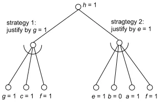
as in backtracking, all “necessities” are enumerated. This leads to a general searching scheme sometimes categorized as AND/OR search in the AI litera-ture [36]. Unlike the decision tree of Section 12.4.1 the AND/OR search tree has two types of nodes, AND-nodes and OR-nodes.
Consider Figure 12.7 . The initial problem to be solved corresponds to the root node in the AND/OR tree. Several strategies are possible. If one strategy is successful the problem is solved. Therefore, the root node is an OR-node. In our example, problem Ï can be solved by strategyÏÔ or Ï4ç . In strategy ÏÔ three sub-problems 9¼ÊG and L arise. All need to be solved, therefore ÏÔ corresponds to an Ïpo L -node. Actually, it turns out that L leads to a
conflict. Hence, strategyÏéÔ is not successful and we considerÏ4ç . This leads
to problemsq and where two strategies exist for problem . This process
continues until the given problems can no longer be decomposed into sub-problems. A closer analysis reveals that no matter what strategy we choose, problem needs to be solved. This yields the implicationsÏsr andurt
t
Ï . Another implication that is perhaps less evident is t
v
t
w
r Ït .
In [26] an AND/OR searching scheme was formulated to derive all neces-sary conditions for the satisfiability of a Boolean function in a Boolean net-work. In contrast to backtrack search (based on a decision tree) that can some-times finish quickly when a sufficient solution exists, AND/OR reasoning can sometimes terminate early when no solution exists. The original motivation was therefore to prove the untestability of stuck-at faults in combinational cir-cuits.
Other applications result from the fact that for an arbitrary node & in the
Boolean network, AND/OR reasoning can derive product terms of the form
À
Â
åwÀ
Å
åCËÌËUËÀ
Í with
$yx2Ô such that ¿ÁÀ
Â
åwÀ
Å
åCËÌËUËÀ
Í
to in [26] as 1-implicants and 0-implicants, respectively. In the special case of
$ ¾6Ô , the technique is called recursive learning and can be used to derive all
implications in a Boolean network (see also Section 12.5.1.1). Besides pruning the search space, implications and implicants in multi-level circuits can be very useful in multi-level logic synthesis [26]. This is based on the same philosophy as for two-level minimization where deduction methods to derive implicants such as iterated consensus have played an important role for a long time.
cdfez 1k`r<Ç `r"rs F k1jgtmoh j r<Çhg|{opq
¡B¢£*}£¡ ¶¶s¨o¤ «¸¦`ì ¤¥¦
·
©ª¯±«¸¦"©
·
This section provides additional detail on techniques to identify simple log-ical relationships and constraints that permit us to simplify the problem in-stances.
ìîíðï~ðï¯ì ïwì õÙõPöøóÙû%âõPûßô ùSòÙúGûUùSò×õ ù úõäûÙû ú öøú%HùSúõPûßô
As already pointed out in previous sections, SAT and ATPG algorithms make extensive use of techniques that evaluate the given set of value assign-ments to the variables (signals) of the CNF-formula or the Boolean network in order to derive further assignments that are uniquely determined by the current situation. In the context of test generation, this process is usually referred to as performing implications. In the terminology of SAT solving methods it is called Boolean constraint propagation (BCP).
It is helpful to use the following classification of implication techniques in Boolean networks.
In a Boolean network, a value assignment at an arbitrary input or output sig-nal of a logic gate follows by simple implication if it is uniquely determined
by previous logic value assignments at other input or output signals of and
by the function of (AND, OR, NOT, NAND, NOR). A simple implication is
a local evaluation of a given gate. Additionally, it is common to distinguish between forward and backward implication, depending on whether the new value assignment is implied at the outputs or the inputs of the considered gate. Figure 12.8 a) and b) show examples of simple forward and backward impli-cations. Simple implications have an equivalent counterpart in the domain of evaluating CNF-formulas. Simple implications in a Boolean network corre-spond to the application of the unit-clause rule as described in Section 12.4.1 if the circuit is modeled by a CNF-formula.
e1U*Ue.I1.
1.]*U1.1.
¡
¢
¢
£
¢
¢
¢
¡
£
¡
£
¡
¡
£
£
¡
£
¡
£
£
¡
¢
¢
¢
¢
¤e¥I¦§1¨©ªU§«U¬®¯§¬®¯¬°1¤.±¬©² ¦³¥¤1¨±§.ª?«6¬®¯§¬®¯¬°1¤.±¬©²
´
´
µ
µ
¶
¶
´
µ
´
µ
¶
¶
´
µ
· ¸¹º
»½¼¾
¿
À Á
Â
ÃeÄÃųÆ.ÇÈÉÃÊ*ËÆ.ÌÍ̳Î*ÍÏUÃ1Ð.ÑIÍÇȳÉÍÐ1Æ.ÑÍÊÌ
!6Ò!
Types of implications in a combinational circuit.
value assignments across several gates along the paths in a circuit; see Figure 12.8 c) and d). Direct implications in a Boolean network correspond to BCP based on the unit-literal rule for a CNF-formula. Note also that the pure-literal rule of Section 12.4.1 has a counterpart in ATPG. Applying the pure-literal rule corresponds to making assignments to so called head objectives [16] that can be identified in Boolean networks by backtracing techniques such as those described in Section 12.5.4.1.
If a value assignment at a given signal is uniquely determined by previ-ous value assignments in the circuit and cannot be implied directly, then it is said to be determined by indirect implication. Figure 12.8 e) shows an exam-ple of an indirect implication. Indirect implications can only be identified by more sophisticated deduction schemes such as the ones already described in Sections 12.4.2.1 and 12.4.2.2, as well as additional ones we describe next. SOCRATES [39] was the first test generator to identify some indirect implica-tions.
ìîíðï~ðï¯ì ïí ÓÔÙò×úÕ4ö:óÖSò×õâúGû#
The goal of identifying logical constraints in ATPG has motivated researchers to study variable probing techniques [39, 40], also known as as static and dy-namic learning. The objective of variable probing is to identify relationships among variables. Consider again the circuit in Figure 12.8e. If the assignment
ɪ¾80 is “probed”, and all direct (forward and backward) implications are
ProbeVariables( ÜØUÙ
Ô
Ù³Ø)
(
ÜÚ ) = simple rules( )
if (is satisfied( )) return ( Ú , true)
if (is unsatisfied( )) return ( , false)
if (Ø6Ù
Ô
ÙØÛÂ)
for (everyàÜ )
Û
Ú
Ü*Ý*Þß]ÞeàÝ
Ý Õ ProbeVariables ($á
Ú á Û à Ý ÜØ6Ù Ô ÙØ á Â )
if (Ý*Þß]ÞeàÝ
Õ true) return (
ÚÑÜÝ*Þß]ÞeàÝ)
Û
Ú
Ü*Ý*Þß]ÞeàÝ
Ý Õ ProbeVariables ($á
Ú á Ûe à Ý ÜeØUÙ Ô Ù³Ø á  )
if (Ý*Þß]ÞeàÝ
Õ true) return (
ÚÑÜÝ*Þß]ÞeàÝ) Ú Õ Ú Ø Û Ú ãâ Ú Ý if (
ÔÚ ) return ( , false)
return (Ú , false)
Gä
Variable probing (St˚almarck’s method).
say thatɪ¾80
;
×è¾80 . Moreover, we can also conclude by applying the law
of contraposition that×¾/Ô
;
ɾ/Ô . Observe that the latter implication is
not readily obtained by a sequence of simple implications but requires an addi-tional concept, in this case, the law of contraposition. Such implications have been referred to as indirect in Section 12.5.1.1 and were called global in [39]. Indirect implications can be identified during a preprocessing phase (i.e. static learning) or during the search phase (i.e. dynamic learning). Note that it is not obvious what signals should be probed in order to identify additional value assignments. Therefore, in static and dynamic learning probing is performed for all unassigned signals of the circuit.
In SAT an example of using variable probing is St˚almarck’s method (SM) [42, 21]. SM is a complete proof procedure for Boolean satisfiability. The core technique of this proof procedure can be interpreted as the recursive appli-cation of variable assignment probing. While static and dynamic learning of [39, 40] apply probing only to all single variables of the circuit SM extends the probing process recursively to all pairs, all triples and so forth.
A recursive version of the variable probing algorithm (adapted from [21]) is illustrated in Figure 12.9. At each depth of the recursive procedure, a set of
conclusions (e.g., unit clauses denoting necessary assignments) is maintained. For every variableÀ the two possible assignments are evaluated and, depending
on the outcome, the problem instance can be deemed satisfied, or currently unsatisfiable.
It is plain to conclude that variable probing with arbitrary depth identifies all necessary assignments. Moreover, if the problem instance is unsatisfiable, variable probing is able to conclude so.
ìîíðï~ðï¯ì ïå ò×óHô#õäö:÷UùSúõäûæÙû çÙû #" õäò ò×ó$ ô õPûUúGû#
èé3ê ëeìíîìïðñ
êò óô
ë.ìõöñ÷.ñùøúüû ýeþÿ
þ ýeþ "!# $%&'()+*,-/.102 !G3
[image:18.612.227.382.103.203.2]AND/OR reasoning tree for46587 .
Figure 12.8e can be used to compare the two techniques. Suppose we want to perform the implications for×Ú¾ÕÔ . First, we consider resolution being applied
to the characteristic CNF-formula of the circuit as given by
ý ¾ ¿äºÃNæ5à ÉÆÂå¿t
t
äºÃ"ÉÆ?Å}å¿tæ5ÃNÉÆ^È}å¿ÉFÃ
t
CÆNfåi¿19KÃ
t
Æ O åw¿
t
9à ÉFÃt CÆ;:}å ¿äºÃ t ÌÆ=<åi¿ tæKà t UÆ;>åw¿ t äºÃNæ5ÃÖÌÆ;?}å¿*à à t×CÆ ÂA@ åw¿ t
à ×CÆ Â? å¿
t
Ã×CÆ ÂãÅ
For better readability of this example the clauses have been numbered as in-dicated by the index at each clause. Performing the implications for ×N¾ Ô
means that we would like to identify all clauses of type ¿×ÚÃ ÀLÆ where À is
some signal of the circuit. Applying resolution to all pairs of clauses results in the following resolvents:
1-4: BCEDGFHDJI KLMN 1-8: BC+DJI O D I ? LMP 1-9: BFHD O D I ? LM J 2-6: B1ICEDQI R D KL MS 2-7: B"I O D ? L MT 3-6: B I FHDUI R D KVL MW 3-9: B1ICED O D ? LMX 4-10: B O D ? D I 4 LZY1[ 5-10: B R D O D I 4 LZY;M 6-12: B1I R D I ? DG4 LZY1Y 7-10: BC+D K D I 4 LZY1N 8-10: B I FHD K D I 4 LZY1P 9-10: B1ICEDGFHD\4 LY J
Clauses that are covered by other clauses can be eliminated. Next, the pairwise comparisons have to be performed for the new clauses too. This procedure has to be continued until no more new clauses are generated. For reasons of brevity we omit these steps but note that the clauses 17 and 20 yield the clause
¿ÉÃ
t×Æ?Å]: . This corresponds to the implication
¿*×¾-ÔUÆpr ¿Áɾ-ÔÌÆ which is
indirect.
We now examine how the same implication can be identified by AND/OR reasoning. Figure 12.10 shows the AND/OR reasoning tree for the assignment
× ¾6Ô . There are two possible strategies to reach this assignment called
justi-fications in [25]. We can justify×¾-Ô by¾6Ô or ¾-Ô (or both). For each
necessary assignment and the implication¿½×Ú¾9ÔÌÆr ¿É¼¾9ÔUÆ is obtained. For
a detailed description of recursive learning and AND/OR reasoning see [26]. The example illustrates some differences between resolution and AND/OR reasoning. Resolution produces all prime clauses for a given CNF-formula. If the CNF-formula represents a multi-level Boolean network we obtain all im-plications and implicants between all nodes in the network. There is usually a tremendous number of such relationships so that only a subset of all clauses can be generated in practice. It is usually hard to develop heuristics such that only those clauses are generated which are relevant for the problem being con-sidered. In the above example, where we are only interested in the implications for×¼¾9Ô it would be sufficient to only generate clauses 17, 20 and 26.
AND/OR-reasoning solves a more specific problem than resolution. It gen-erates all implicants for a particular target line in a multi-level circuit, such as
× in the above example, i.e., it only generates all clauses of the form ¿*×Ã1ËÌËUËÆ
or¿ ×FÃ ËUËÌËÆ . Therefore, it can be more efficient than resolution if our interest
is in implicants for a specific target line or in implications for a specific set of value assignments in a multi-level circuit.
In general, however, both, resolution and AND/OR-reasoning are fairly ex-pensive methods. They should only be used in SAT or ATPG when other less expensive methods fail.
ìîíðï~ðï¯ì ï¨ñ ù4õ4õäöÂõÕ Uú%'×ö ×ûÙö_^ßô úô8`åõPò ÷UûUúbaä÷Uó ô óûàô úGùSúdc HùSúõPû
In ATPG, the requirement of fault observability can result in additional search constraints called unique sensitization. This is based on a topologi-cal analysis conducted on a representation of the circuit as a directed acyclic
graph (DAG).
Note that a fault signal can only propagate through a specific gate if the other inputs of that gate are set to specific values (1 for AND-gates, 0 for OR-gates). This is called sensitization of a gate. A topological analysis of the circuit graph can often identify sets of gates through which the fault signal must propagate in order to reach an output [16], [24].
As an example, consider the circuit in Figure 12.2. For a target fault at sig-nalæ it is obvious that the fault signal must propagate through gates e ,É and × . In the DAG representation of the circuit these nodes are called
¡B¢£*}£¢ · ±¯ ¤ë5 3Ú¯¨s¦"«¸¦`ì ¹ª» ¤¥¦"´³º«Ò¤ © ±¦"±³(»
·
«
·
There exist a variety of dedicated techniques for pruning the search space in backtrack search algorithms. Most of these techniques come into play when-ever conflicting conditions are identified and are equally applicable in SAT and ATPG tools.
To explain these techniques, it is useful to note the following additional definitions relating to the backtrack search process (see Section 12.4.1). A decision level is associated with each variable selection and assignment. The first variable selection corresponds to decision level 1. For each new decision, the decision level is incremented by 1. The application of the unit clause rule yields variables whose value is implied. The unit clauseÐ5à that implies the
assignment of a variable À to value fB¿ÀLÆ is referred to as the antecedent of À , g}¿ÀLÆ . The decision level of each implied variable À , h¿ÀCÆ , is given by the
highest decision level of the variables that directly makeÐ a unit clause (before À is assigned). The notation À1¾ifB¿ÁÀCÆ=j/h¿ÀLÆ/7kg}¿ÀLÆ is used to denote that
variableÀ is assigned valuefB¿ÀCÆ with decision levelh¿ÀCÆ and antecedentgf¿ÁÀCÆ .
When a variable Û is a decision variable, and so with no antecedent, then gf¿ÛºÆ¾mlonAp .
For example, to compute the decision level of a variableÀ , implied due to a
unit clauseÐ à , the following formula can be applied:
h ¿ÁÀCƾ
%
äiÀÎh¿&iÆ7H¿& . ÐKàwÆrq¿&ts¾ ÀCÆÓ
Observe that the unit clauseÐKà becomes satisfied as soon as À is assigned its
implied valuefB¿ÀLÆ . Moreover, observe that decision levels, although strictly
not necessary for implementing the techniques described below, significantly simplify the process of explaining those techniques.
ìîíðï~ðïíïwì % ö P÷àôðóüòÙó'%âõPòÕ UúGû#
uUu uUu uUu
vUv vUv vUv
wUw wUw wUw xUx xUx
xUx yUy
yUy yUy zUz zUz zUz
{U{U{ {U{U{ {U{U{ |U| |U| |U|
}U}U} }U}U} }U}U} ~U~ ~U~ ~U~
UU UU UU
U U U
d = 1
e = 1 b = 1 c = 0
conflict
f = 0 a = 0
!åG
Example of clause recording.
Consider the following example CNF formula:
½¾¿äºÃ"æÇÆKåi¿ÄæÃ9ÃeÆêå¿Äæ5ÃÖUÆêåë¿ÁÄEe Ã"Ä }Ã"ÉÆBåÌåUå
Moreover assume the sequence of decision assignments9¾ 0 andɾ 0 .
In this case, the order of decisions is9è¾ 0 first (hence, 9è¾ 0Jj$Ô/7 lonAp ),
and ɾ 0 next (hence, ɾ 0j çü76lnp ). Let us further assume a few
other decision assignments, to be used in the next section, and finally assume the decision assignmentäF¾06jß7lonAp . The obtained implication sequence
resulting in a conflict is shown in Figure 12.11.
By inspection it is straightforward to conclude that¿19}¾80wÆq ¿ÁÉÚ¾80ÒÆqF¿ä¾ 0wÆr ¿½ ¾ 0wÆ . Since the objective is to have ½ ¾2Ô , then one immediately
concludes that ½ r ¿9fÃqɪà äÆ . Hence ¿19}à ɪà äiÆ denotes a new clause
that can be added to the CNF formula (i.e. it can be recorded). Moreover,
¿19à ɼà äiÆ can be viewed as an explanation of this conflict, and so enables
avoiding the same conflict to occur again during the search.
As the example illustrates, relevant assignments are split into assignments at the current decision level and assignments at lower, i.e. earlier, decision levels. Assignments at lower decision levels are recorded, whereas assignments at the current decision level are used to trace the causes of the conflict to the decision assignment. The resulting set of assignments (all at lower decision levels with the exception of the decision variable) are used to specify the clause to be recorded [33].
In general it is not feasible to record the explanations for all conflicting conditions identified during the search. As a result, it is often the case that large clauses with a number of literals above a certain size are eventually deleted during the subsequent search [33]. Large clauses can be deleted whenever they become unresolved during the subsequent search.
infor-UU UU UU UU UU UU UU UU UU UU UU UU U U U U U U U U U U U U UU UU UU U U U UU UU UU UU UU UU U U U U U U U U U U U U UU UU UU U U U c = 0
g = 1 b = 1
f = 0
f = 0 c = 0
d = 1
e = 1 conflict a = 1
!å!
Example of non-chronological backtracking.
mation is used to reduce the amount of search for the current and subsequent target faults.
ìîíðï~ðïíïí ûßõPû?%&Öò×õPûàõäöÂõÕ Öú%Ùöp%6 Öù òÕ%6 Öúû
The backtrack search procedure, as described in Section 12.4.1, implements chronological backtracking, where backtracking is always performed to the most recent decision assignment which has not yet been toggled by a previous backtrack step. In general, for real-world problem instances, chronological backtracking can perform poorly when compared with alternative approaches, namely non-chronological backtracking, where the search algorithm can back-track to decision assignments which are in fact deemed relevant for each iden-tified conflict.
It is interesting to observe that the utilization of clause recording (described in the previous section) provides the necessary information for implementing non-chronological backtracking. The remainder of this section illustrates one possible approach for implementing a non-chronological backtracking search strategy. A detailed explanation of the implementation of non-chronological backtracking is available in [33].
In order to illustrate how non-chronological backtracking can be imple-mented assume an augimple-mented version of the example in the previous section,
½ ¾ ¿ä Ã"æÇÆêåë¿ÁÄæÃ9áeiÆKåi¿ÄæKà UÆåw¿ÄEeºÃNÄ ]ÃNÉÆåw¿ÄäºÃ CÆ5å ¿ÄKÜÃNæÇÆ5å¿ÁÄ ×ÃÈVÆ5åw¿ÄåCã¢Æåw¿äºÃ9ÃNÉÆÇÊ
where the clause recorded as a result of the conflict analyzed in the previous section is already shown. Moreover, assume the decision assignments9¾ 0 , ɾ 0 , ×1¾ 0 and F¾ 0 . The implication sequence that results from this
scenario is shown in Figure 12.12. Note that the previous decision variableä
is now implied by the just derived conflict clause ¿äFä9ÃÉÆ, and that the
new implication sequence leads to another conflict. Analysis of this new con-flict readily yields a new clause ¿19]Ã1ÉHÆ , which indicates that backtracking is
irrel-¥U¥U¥ ¥U¥U¥ ¥U¥U¥ ¦U¦ ¦U¦ ¦U¦ §U§U§ §U§U§ §U§U§ ¨U¨U¨ ¨U¨U¨ ¨U¨U¨ ©U© ©U© ©U© ªUª ªUª ªUª «U« «U« «U« ¬U¬ ¬U¬ ¬U¬ U U U ®U® ®U® ®U® ¯U¯U¯ ¯U¯U¯ ¯U¯U¯ °U° °U° °U° ±U± ±U± ±U± ²U² ²U² ²U² ³U³U³ ³U³U³ ³U³U³ ´U´ ´U´ ´U´ µUµ µUµ µUµ ¶U¶ ¶U¶ ¶U¶ ··· ¸¸ c = 0
a = 0 b = 1
g = 0
h = 0
f = 0 conflict
i = 1
¹»º¼b½¾1¿EÀÂÁÄÃÅÀGÃbÃ
Example of unique implication point.
evant for the two most recent conflicts, and that backtracking to one of these two decision assignments would not eliminate these conflicts. To remove the conflicting conditions the backtrack search algorithm needs to backtrack to one of the decisions indicated by Æ19ÈÇÊÉÌË . In general the backtracking step is
performed to the most recent decision, in this caseÉJÍmÎ .
In ATPG the utilization of non-chronological backtracking search strategies was initially outlined in [29, 30], and detailed and implemented in [31]. Inter-estingly, the work of [15, 17] did not utilize non-chronological backtracking, and the work of [29, 30, 31] did not consider search equivalence or dominance conditions.ÏÑÐ
ÒÔÓÕÒ
Ð
ÒÅÖ ×ÙØÈÚÛØEÜkÝÙÞ\ßàØ ]á
ÝGâHØÈãäÚ ØåÝæ×ÙÞ çÂÞéèêÝæÞGãêëGÞGçbì/ë Ø ç=íîïÚ çbß6Ýñð6çbò/Þóîoò/ç=ÞGðoâ
Besides the creation of conflict clauses, the ability to backtrack non-chrono-logically, and the deletion of large clauses, a few additional search pruning techniques have been proposed that also build upon clause recording.
Relevance-based learning [5] consists of extending the life-span of clauses, by deleting unresolved recorded clauses only after a certain number of literals becomes unassigned. We should note that relevance-based learning is often integrated with deletion of large clauses, and so large clauses are only deleted when a certain number of literals becomes unassigned.
Unique implication points denote dominators [45] in the graph of implica-tions of decision assignments with respect to identified conflicts. Unique impli-cation points represent variable assignments which, by themselves, can trigger sequences of implied assignments that yield the same conflicts. Consider the following CNF formula,
Æ1ôrÇUõËö=Æ1÷Eõ_ÇUøÇU÷ùÕË_ö=Æ1÷Eõ_ÇQ÷EúûË_ö]Æù+ÇQúEÇUüAË_ö=Æ1÷EüÇUýË_ö=Æ1÷EüÇUþVË_ö=Æ1÷EýrÇU÷Eþ»ÇQÉÌË
and the sequence of decision assignments ø8ÍÿÎ , É ÍÿÎ and ô ÍÎ . The
resulting implied assignments are shown in Figure 12.13. The clause recording procedure outlined in section 12.5.2.1 would identify the new clauseÆ1ô»ÇÙøVÇÙÉ Ë .
However, noting that the implied assignmentü6Í
conflict, one can create instead two clauses, namelyÆ1÷Eü»Ç¡ÉÌË andÆôÇ£ø Ç£üAË .
After erasing the most recent sequence of implied assignments and decision assignmentÆô ÍÎ Ë , a new unit clause is identified Æ1÷EüÌÇ¡ÉÌË and the resulting
implied assignments includeürÍmÎ andôæÍ
, that result from the two recorded clauses. Observe that the original procedure would only implyôæÍ
from the sole recorded clause.
)*+$,+.- /10325468796:<;5=>;@? 034BAC25;5=ED1:F4BG
The backtrack search procedure can be augmented with different techniques described in previous sections, namely resolution, AND/OR reasoning and variable probing [32]. The integration of these techniques with other search pruning techniques used in backtrack search is technically challenging, be-cause each derived necessary assignment must be explained in terms of newly added clauses. Interestingly, the identification of explanations for the nec-essary assignments identified with resolution, AND/OR reasoning (recursive learning) and variable probing (St˚almarck’s method), provides another mech-anism for clause recording, and consequently allows establishing new pruning techniques that differ fundamentally (due to clause recording) from the original ones.
Recent work in SAT has involved formula simplification techniques [34] and search strategies based on randomization with restarts [19, 4]. Formula simplification establishes conditions for removing variables and inferring new clauses. Randomization with restarts allows the search process to consider al-ternative search paths after a pre-determined number of backtracks is reached.
)*+$,+.H IJ6LKM;@AC25=>;@? 254:<6L=G03=EAJG ÏÑÐ
ÒÔÓÕÒONHÒ
Ï
âÕØåÝæ×Ùß'PêîÛÝkðQPéâ8ç=ÞêÝñð6îoè
The performance of test generators can be greatly influenced by the use of backtracing procedures as has been shown in the FAN-algorithm [16]. Their goal is to effectively drive the test generation process towards certain objectives [16]. The objectives result from the general strategy to move the D-frontier towards the primary outputs and the J-frontier towards the primary inputs.
In [16] an objective is defined as a triple Æ1É(RS(TÆ1ÉÌËURSWVdÆÉ ËÂË where É is a
signal in the Boolean network, S
T
Æ1ÉÌË is an integer number expressing how
strongly the logic value 0 is required at É and S V Æ1ÉÌË is an integer number
expressing how strongly the logic value 1 is required atÉ . The initial objectives
\
\
] ^
_a`babdcfehgXijlkmidnoprq(sutwvyxzsu{a|t}sa~~md~vX|lm{ zzuwal
hu(
$
d
&z$wa}u
$m u¡¢ £¤¥$¦§¨©uª«
¬m®$¯.°±.²m³
´
µ ¶·¸h¹$º»¼m½u¾¿ ÀÁÂ$ÃÄÅÆuÇÈ
ÉÊmËuÌÍmÎuÏÐ
Ñ
ÒCÓÔhÕ$Ö×ØmÙuÚÛ ÜÝzÞ$ßUàámâXãä åæmç$è.éuêëíìîmïuð.ñòXóô
¹»º¼b½¾1¿EÀÂÁÄÃÅÀõÃ
Backpropagation of objectives in FAN.
The main goal of backtracing is the early identification of conflicts. If a fanout pointÉ is reached with contradictory requirements, i.e.,S(TÆ1ÉÌË'ö£Î and S V ÆÉ Ë÷ö
, the backtracing process stops and an optional value assignment is made at É , i.e., a decision is made at at this fanout point and inserted in
the decision tree. If no conflict occurs backtracing continues until the primary inputs are reached and the numbersS(TÆ1ÉÌË andSWVÆ1ÉÌË indicate what value
as-signment should be made to reach the objectives of the test generation process. Importantly, as long as backtracing produces fanout points with contradictory requirements these are always chosen first for decision making so that conflicts are detected as early as possible and backtracks are avoided. An improvement to this scheme based on single path backtracing has recently been proposed in [22].
Note that this is related to the general strategy of selecting the non-unate variables in two-level circuit representations as decision points in SAT solv-ing or tautology checksolv-ing. If we formulated the objectives of a FAN-based test generation procedure by a Boolean function to be satisfied, the conflict-ing variables would correspond to non-unate variables of this characteristic function. This explains why backtracing is very important. It is the basic in-strument to incorporate a strategy also known as unate recursive paradigm [6] into a Boolean decision making procedure operating on multi-level Boolean networks. Therefore, backtrace procedures represent an integral part of almost all modern ATPG tools.
ÏÑÐ ÒÔÓÕÒONHÒ
Ð
á
×ÙÝæÞ\ßùPGç=Þ\èúPGØÈëG×ÙçbâHð6çbßoâ ç=Þäß6ÞüûWýÄâHÝñð
One of the most important but least understood aspects of SAT algorithms is how to choose the next decision variable at each branching point. Various au-thors [28, 23, 8, 13] have experimented with many different branching schemes with different degrees of success. Gomes et al. provide an excellent review of this subject [20].
Despite the effort spent on decision schemes, it is still unknown what prop-erties make a particular decision scheme better than others. Current decision schemes are mostly based on intuition and empirical results. Usually, a good decision scheme for a certain class of problems may not be good for others. Thus, it is very hard to determine which decision scheme should be used for a certain class of problems.
Traditional decision schemes generally emphasize the quality of the deci-sion, e.g., minimization of the total number of decisions required to solve cer-tain problems. Although the number of decisions is a straightforward metric to compare different strategies – fewer decisions ought to mean smarter deci-sions – it is not the only metric, since not all decideci-sions yield an equal number of BCP operations. As a result, a shorter sequence of decisions may actually lead to more BCP operations than a longer sequence of decisions. Besides, traditional decision schemes usually involve updating some statistics dynam-ically, and thus are computationally expensive. As the deduction process be-comes more and more optimized, the time spent on decision making in a SAT solver becomes non-negligible. Therefore, it is important to keep the decision-making overhead to a minimum, while maintaining the quality of the branching heuristic. Recently Chaff has introduced a very low overhead decision scheme referred to as variable state independent decision strategy (VSIDS) [35]. The emphasis here is on minimizing computation overhead for decision state main-tenance in change of variable state during branching and backtracking.
þÿ
)*+! +) A#" KJ: G4%$ K0ZKMIKFG4 G0/16MK ?<4 ÏÑÐ
Ò'&ÕÒ
Ï
Ò
Ï
âHîÛÝæ×GâHØ£íÝkðï×æç)(ó×ÙØÈî6×ÙØñâHØÈÞGðÛÝñð6çbò Þ
The simplest and currently most widely used data structure is to represent the clauses in a sparse matrix. Each clause stores a vector of the literals in it, and some statistical data, e.g., the number of total literals, the number of free literals, etc. Each variable may keep a list of all its occurrences (as in GRASP [33]) or some of its occurrence (as in SATO [47] or Chaff [35]) in the clause database.
*,+.-0/21435,6872943:<;=*?>@
The most straightforward BCP method operating on a sparse matrix clause database is to keep three counters for each clause: the total number of literals, the number of literals evaluating to 1, and the number of literals evaluating to 0. The first counter is constant during the entire lifetime of the clause. The other two counters are updated whenever the related variable is set/unset to a value. The status of a clause - conflict, satisfied or unit - can be determined by these three counters (e.g., GRASP [33] ). An efficient variation of this method eliminates the need to store the number of literals that evaluate to 1 ( e.g., relsat [5] ).
>+BAC/2143D5E6.729F3D:G;*>H@
A more efficient way to implement the BCP op-eration is proposed by SATO [46]. Although the data structure in SATO is also based on sparse matrices, it determines the status of the clauses in a different way. Each clause has two pointers: Head and Tail to point to its first and last unassigned literals. Instead of keeping track of all the literal occurrences -for each variable, the Head List is a collection of its occurrences as the first unassigned literal in the clauses, and the Tail List is a collection of its occur-rences as the last unassigned literal in the clauses. Starting from a variable, one needs to only visit the clauses that have this variable as their Head/Tail. Unit clauses and conflict clauses are detected by examining the relative positions of the Head and Tail pointer of the clauses.
The key advantage of this algorithm is that whenever a variable changes state, only the clauses in the Head/Tail list for this variable will be visited. When we move the Head/Tail literals, it is possible that we will encounter a value 1 literal very early if the clause is satisfied. Whenever a search for the next Head or Tail encounters a literal with value 1, the Head or Tail of the clause will stop to be active, thus eliminating the need to update the status of the clause in the future.
“watched” literals have the property of being the last to be assigned to value 0 if the clause is not satisfied. Each variable only keeps a list of all its “watched” literals. In practice, the “watched” literals of the two different phases (comple-mented and uncomple(comple-mented) are kept in separate arrays. Whenever a variable becomes assigned, Chaff traverses through all the “watched” literals of this variable evaluating to 0.
Chaff’s BCP algorithm has all the advantages of SATO’s algorithm during the deduction procedure. Moreover, during backtracking, undoing assignments does not require a change in the states of the clauses, i.e. there is no need to change the “watched” literals. The reason is that the “watched” literals have the property of being the last to be assigned value 0 if the clause is not satisfied, therefore, they will be the first to become unassigned if the clause is free again. Therefore, un-assigning variable assignments in backtracking is very cheap. This is a very significant performance advantage.ÏÑÐ
Ò'&ÕÒ
Ï
Ò
Ð
ç=íî6ÚÛçbßàçÂð¤ãÙÝkðÛÝ âHð6×/ë\ßàð6ëG×ÙØñâ
Besides the sparse matrix clause database representation, there are some other data structures that have been proposed in the literature for storing the clauses.
A version of SATO uses a data structure called a trie to store the clause database. A trie is a ternary tree. Each internal node in the trie structure is a variable index, and its three leaf edges are labeled Pos, Neg and DC respec-tively for positive, negative and don’t care. A leaf node in a trie is either True or False. Each path from root of the trie to a True leaf represents a clause. A trie is said to be ordered if for every internal node V, Parent(V) has a smaller variable index than the index of variable V. The ordered trie structure has the nice property of being able to detect duplicate and tail subsumed clauses of a database quickly. A clause is said to be tail subsumed by another clause if its first portion of the literals (a prefix) is also a clause in the clause database. For example, Æ1ôoÇõEÇøË is tail subsumed byÆ1ôoÇõË .
Intuitively an ordered trie has some similarity with binary decision dia-grams, i.e. easy sharing of common parts. This has naturally led to the ex-ploration of other decision diagram style set representations. Chatalic [10] and Aloul [3] have both experimented with using zero-suppressed binary decision diagrams (ZBDD) to represent the clause database. A ZBDD representation of the clause database can detect not only tail subsumption but also head sub-sumption. Both authors report significant compression of the clause database for certain classes of problems.
KML
K
N
N
L
O
N
L
KL
N
OPL
K
QSRUTUVWQYX[Z]\!^QY_U`badcegf hikjlYm[noYm[p]q!roYst'lduvgwxvDy
¹»º¼b½¾"¿ À=ÁbÃÔÀdzÂÃ
Implication graph for clauses with two and three literals.
)*+! +$* ?<6MKM7B2 $1K 0ZK G036J: AC03:F6M4BG|{Z/ 6 I AC7
In the context of CNF-based ATPG algorithms implication graphs[9, 44] have been proposed as specific data structures for efficient implementations of implication techniques. The implication graph of [44] is a directed graph
},~
ÍäÆP RGË where the vertex set is partitioned into a set of signal nodes
and a set of -nodesB . Signal nodes represent the encoding bits of a signal
. For simplicity, we assume a three-valued logic alphabet ÎR
R . In this
case, for each clause variable
two nodes,
and
are introduced in
}
~
. If we assign in the circuit
Í
or
Í Î then in } ~
node
or
, respectively, is said to be set. EachS -ary clause in the characteristic CNF of the circuit is
represented by S associated -nodes in } ~
and SB edges connecting the
-nodes with the signal -nodes for the clause variables. The implication graph for a binary and ternary clause are shown in Figure 12.15.
Direct implications can be performed in
} ~
by setting signal nodes accord-ing to the followaccord-ing rule:
Starting from an initial set of set signal nodes, all immediate successor nodes
are set if node
is an -node and all its immediate predecessors are set, or
if node
is a signal node and at least one immediate predecessor is set. This rule is applied repeatedly until no additional node can be set. A logic inconsistency occurs if there is a signal
in the graph such that both
and
are set.
þÿ < G<g
¢¡ £
The first complete method to generate test vectors for single stuck-at faults was the famous D-algorithm proposed by Roth [37]. Goel [18] formulated test generation as backtrack search for the input variables of the circuit. In his test generator PODEM he introduced the general ATPG procedure as was dis-cussed in Section 12.3. Important refinements to this procedure were proposed by Fujiwara and Shimono [16]. Their ATPG tool FAN was the first to incor-porate a sophisticated backtracing procedure as well as unique sensitization. Another significant step was made in SOCRATES [39] where it was shown by Schulz et al. that the ATPG process can greatly benefit from the identification of indirect implications.
With respect to the SAT domain, the first algorithm was the well-known Davis-Putnam procedure [12], which is based on the application of iterated resolution. Shortly afterwards, the first backtrack search algorithm was pro-posed [11], which is commonly known as the Davis-Logemann-Loveland (DLL) procedure. Recent years have seen significants improvements being made to the basic DLL procedure, with the introduction of non-chronological back-tracking, clause recording and several other very effective search pruning tech-niques [33, 5]. More recently, the implementation of efficient SAT solvers has been subject to key improvements [35].
One may expect that further progress in the area of SAT and ATPG is very hard after decades of research. However, innovation could result particularly from combinations of search pruning techniques that have so far been consid-ered independently from each other. As already pointed out in Section 12.5.3, the concept of clause recording that has been applied in backtrack search and AND/OR reasoning could be extended to other reasoning schemes like resolu-tion or variable probing, or even approaches using a mix of backtrack search and reasoning schemes.
ATPG and SAT continuously conquer new application domains. Specific applications require specific heuristics. As an example, SAT-based property checking recently became an intensive field of research and it is a challenging task to adapt SAT algorithms to traversing sequential circuits. Therefore, as with SAT and combinational ATPG today, in the near future, we may see a unification process of SAT and sequential ATPG, promising not only a unified terminology but also substantially more powerful tools.
¥¤8¦¤§¤.¨©.¤.ª
[1] M. Abramovici, M. Breuer, and A. Friedman, Digital Systems Testing and Testable
[2] S. Akers, “A logic system for fault test generation,” IEEE Trans. on Comp., vol. 25, pp. 620–630, June 1976.
[3] F. A. Aloul and K. A. Sakallah, “SAT using ZBDDs,” in Dagstuhl Seminar 01051 on
Computer Aided Design and Test – BDDs versus SAT, Schloss Dagstuhl, Germany, Jan
28-Feb 2 2001.
[4] L. Baptista and J. P. Marques-Silva, “Using randomization and learning to solve hard real-world instances of satisfiability,” in Proc. Intl. Conf. on Principles and Practice of
Constraint Programming, September 2000.
[5] R. Bayardo Jr. and R. Schrag, “Using CSP look-back techniques to solve real-world SAT instances,” in Proc. Natl. Conf. on Artificial Intelligence, pp. 203–208, 1997.
[6] R. K. Brayton, G. D. Hachtel, C. T. McMullen, and A. L. Sangiovanni-Vincentelli, Logic
Minimization Algorithms for VLSI Synthesis. Kluwer Academic Publishers, 1984.
[7] F. Brown, Boolean Reasoning – The Logic of Boolean Equations. Kluwer Academic Publishers, 1990.
[8] M. Buro and H. Kleine-Buning, “Report on a SAT competition,” in Technical report,
University of Paderborn, 1992.
[9] S. Chakradhar, V. D. Agrawal, and S. Rothweiler, “A transitive closure algorithm for test generation,” IEEE Trans. on CAD, vol. 12, pp. 1015–1028, July 1993.