An Empirical Study of Semi supervised Structured Conditional Models for Dependency Parsing

An Empirical Study of Semi-supervised Structured Conditional Models

for Dependency Parsing

Jun Suzuki, Hideki Isozaki NTT CS Lab., NTT Corp.

Kyoto, 619-0237, Japan [email protected] [email protected]

Xavier Carreras, and Michael Collins MIT CSAIL

Cambridge, MA 02139, USA [email protected] [email protected]

Abstract

This paper describes an empirical study of high-performance dependency parsers based on a semi-supervised learning ap-proach. We describe an extension of semi-supervised structured conditional models (SS-SCMs) to the dependency parsing problem, whose framework is originally proposed in (Suzuki and Isozaki, 2008). Moreover, we introduce two extensions re-lated to dependency parsing: The first ex-tension is to combine SS-SCMs with an-other semi-supervised approach, described in (Koo et al., 2008). The second exten-sion is to apply the approach to second-order parsing models, such as those de-scribed in (Carreras, 2007), using a two-stage semi-supervised learning approach. We demonstrate the effectiveness of our proposed methods on dependency parsing experiments using two widely used test collections: the Penn Treebank for En-glish, and the Prague Dependency Tree-bank for Czech. Our best results on test data in the above datasets achieve 93.79% parent-prediction accuracy for En-glish, and 88.05% for Czech.

1 Introduction

Recent work has successfully developed depen-dency parsing models for many languages us-ing supervised learnus-ing algorithms (Buchholz and Marsi, 2006; Nivre et al., 2007). Semi-supervised learning methods, which make use of unlabeled data in addition to labeled examples, have the po-tential to give improved performance over purely supervised methods for dependency parsing. It is often straightforward to obtain large amounts of unlabeled data, making semi-supervised ap-proaches appealing; previous work on

semi-supervised methods for dependency parsing in-cludes (Smith and Eisner, 2007; Koo et al., 2008; Wang et al., 2008).

In particular, Koo et al. (2008) describe a semi-supervised approach that makes use of clus-ter features induced from unlabeled data, and gives state-of-the-art results on the widely used depen-dency parsing test collections: the Penn Tree-bank (PTB) for English and the Prague Depen-dency Treebank (PDT) for Czech. This is a very simple approach, but provided significant perfor-mance improvements comparing with the state-of-the-art supervised dependency parsers such as (McDonald and Pereira, 2006).

This paper introduces an alternative method for semi-supervised learning for dependency parsing. Our approach basically follows a framework pro-posed in (Suzuki and Isozaki, 2008). We extend it for dependency parsing, which we will refer to as a Semi-supervised Structured Conditional Model (SS-SCM). In this framework, a structured condi-tional model is constructed by incorporating a se-ries of generative models, whose parameters are estimated from unlabeled data. This paper de-scribes a basic method for learning within this ap-proach, and in addition describes two extensions. The first extension is to combine our method with the cluster-based semi-supervised method of (Koo et al., 2008). The second extension is to apply the approach to second-order parsing models, more specifically the model of (Carreras, 2007), using a two-stage semi-supervised learning approach.

We conduct experiments on dependency parsing of English (on Penn Treebank data) and Czech (on the Prague Dependency Treebank). Our experi-ments investigate the effectiveness of: 1) the basic SS-SCM for dependency parsing; 2) a combina-tion of the SS-SCM with Koo et al. (2008)’s semi-supervised approach (even in the case we used the same unlabeled data for both methods); 3) the two-stage semi-supervised learning approach that

corporates a second-order parsing model. In ad-dition, we evaluate the SS-SCM for English de-pendency parsing with large amounts (up to 3.72 billion tokens) of unlabeled data .

2 Semi-supervised Structured

Conditional Models for Dependency Parsing

Suzuki et al. (2008) describe a semi-supervised learning method for conditional random fields (CRFs) (Lafferty et al., 2001). In this paper we extend this method to the dependency parsing problem. We will refer to this extended method as Semi-supervised Structured Conditional Mod-els (SS-SCMs). The remainder of this section de-scribes our approach.

2.1 The Basic Model

Throughout this paper we will usexto denote an input sentence, and yto denote a labeled depen-dency structure. Given a sentencexwithnwords, a labeled dependency structureyis a set ofn de-pendencies of the form (h, m, l), whereh is the index of the head-word in the dependency, m is the index of the modifier word, and lis the label of the dependency. We useh = 0 for the root of the sentence. We assume access to a set of labeled training examples, {xi,yi}Ni=1, and in addition a

set of unlabeled examples,{x0

i}Mi=1.

In conditional log-linear models for dependency parsing (which are closely related to conditional random fields (Lafferty et al., 2001)), a distribu-tion over dependency structures for a sentence x

is defined as follows:

p(y|x) = _Z(1_x)exp{g(x,y)}, (1)

where Z(x) is the partition function, w is a pa-rameter vector, and

g(x,y) = X (h,m,l)∈y

w·f(x, h, m, l)

Here f(x, h, m, l) is a feature vector represent-ing the dependency(h, m, l)in the context of the sentence x (see for example (McDonald et al., 2005a)).

In this paper we extend the definition ofg(x,y)

to include features that are induced from unlabeled data. Specifically, we define

g(x,y) = X (h,m,l)∈y

w·f(x, h, m, l)

+ X

(h,m,l)∈y

k

X

j=1

vjqj(x, h, m, l). (2)

In this modelv1, . . . , vkare scalar parameters that

may be positive or negative; q1. . . qk are

func-tions (in fact, generative models), that are trained on unlabeled data. Thevj parameters will dictate

the relative strengths of the functionsq1. . . qk, and

will be trained on labeled data.

For convenience, we will use vto refer to the vector of parametersv1. . . vk, andqto refer to the

set of generative modelsq1. . . qk. The full model

is specified by values for w,v, and q. We will write p(y|x;w,v,q) to refer to the conditional distribution under parameter valuesw,v,q.

We will describe a three-step parameter estima-tion method that: 1) initializes the q functions (generative models) to be uniform distributions, and estimates parameter valueswandv from la-beled data; 2) induces new functionsq1. . . qkfrom

unlabeled data, based on the distribution defined by thew,v,qvalues from step (1); 3) re-estimates

w and v on the labeled examples, keeping the

q1. . . qk from step (2) fixed. The end result is a

model that combines supervised training with gen-erative models induced from unlabeled data.

2.2 The Generative Models

We now describe how the generative models

q1. . . qk are defined, and how they are induced

from unlabeled data. These models make direct use of the feature-vector definitionf(x,y)used in the original, fully supervised, dependency parser.

The first step is to partition the d fea-tures in f(x,y) into k separate feature vectors,

r1(x,y). . .rk(x,y) (with the result thatf is the

concatenation of thekfeature vectorsr1. . .rk). In

our experiments on dependency parsing, we parti-tionedf into up to over140separate feature vec-tors corresponding to different feature types. For example, one feature vectorrj might include only

those features corresponding to word bigrams in-volved in dependencies (i.e., indicator functions tied to the word bigram(xm, xh)involved in a

de-pendency(x, h, m, l)).

We then define a generative model that assigns a probability

q0

j(x, h, m, l) = dj

Y

a=1

θrj,a(x,h,m,l)

j,a (3)

to thedj-dimensional feature vectorrj(x, h, m, l).

they form a multinomial distribution, with the con-straints that θj,a ≥ 0, and Paθj,a = 1. This

model can be viewed as a very simple (naive-Bayes) model that defines a distribution over fea-ture vectorsrj ∈Rdj. The next section describes

how the parametersθj,a are trained on unlabeled

data.

Given parametersθj,a, we can simply define the

functionsq1. . . qkto be log probabilities under the

generative model:

qj(x, h, m, l) = logqj0(x, h, m, l)

=

dj

X

a=1

rj,a(x, h, m, l) logθj,a.

We modify this definition slightly, be introducing scaling factorscj,a >0, and defining

qj(x, h, m, l) = dj

X

a=1

rj,a(x, h, m, l) logθ_cj,a j,a (4)

In our experiments, cj,a is simply a count of the

number of times the feature indexed by(j, a) ap-pears in unlabeled data. Thus more frequent fea-tures have their contribution down-weighted in the model. We have found this modification to be ben-eficial.

2.3 Estimating the Parameters of the Generative Models

We now describe the method for estimating the parameters θj,a of the generative models. We

assume initial parameters w,v,q, which define a distribution p(y|x0

i;w,v,q) over dependency

structures for each unlabeled examplex0

i. We will

re-estimate the generative modelsq, based on labeled examples. The likelihood function on un-labeled data is defined as

M

X

i=1

X

y p(y|x 0

i;w,v,q)

X

(h,m,l)∈y

logq0_j(x0_i, h, m, l),

(5) whereq0

j is as defined in Eq. 3. This function

re-sembles theQfunction used in the EM algorithm, where the hidden labels (in our case, dependency structures), are filled in using the conditional dis-tributionp(y|x0

i;w,v,q).

It is simple to show that the estimatesθj,a that

maximize the function in Eq. 5 can be defined as follows. First, define a vector ofexpected counts

based onw,v,qas

ˆ rj =

M

X

i=1

X

y p(y|x 0

i;w,v,q)

X

(h,m,l)∈y

rj(x0i, h, m, l).

Note that it is straightforward to calculate these ex-pected counts using a variant of the inside-outside algorithm (Baker, 1979) applied to the (Eisner, 1996) dependency-parsing data structures (Paskin, 2001) for projective dependency structures, or the matrix-tree theorem (Koo et al., 2007; Smith and Smith, 2007; McDonald and Satta, 2007) for non-projective dependency structures.

The estimates that maximize Eq. 5 are then

θj,a= Pdˆrjj,a

a=1ˆrj,a

.

In a slight modification, we employ the follow-ing estimates in our model, whereη >1is a pa-rameter of the model:

θj,a = (η−1) + ˆrj,a

dj×(η−1) +Pdaj=1rˆj,a

. (6)

This corresponds to a MAP estimate under a Dirichlet prior over theθj,aparameters.

2.4 The Complete Parameter-Estimation Method

This section describes the full parameter estima-tion method. The input to the algorithm is a set of labeled examples {xi,yi}Ni=1, a set of

unla-beled examples {x0

i}Mi=1, a feature-vector

defini-tionf(x,y), and a partition offintokfeature vec-tors r1. . .rk which underly the generative

mod-els. The output from the algorithm is a parameter vectorw, a set of generative modelsq1. . . qk, and

parametersv1. . . vk, which define a probabilistic

dependency parsing model through Eqs. 1 and 2. The learning algorithm proceeds in three steps:

Step 1: Estimation of a Fully Supervised Model. We choose the initial value q0 _{of the}

generative models to be the uniform distribution, i.e., we set θj,a = 1/dj for allj, a. We then

de-fine the regularized log-likelihood function for the labeled examples, with the generative model fixed atq0_{, to be:}

L(w,v;q0_{) =}Xn

i=1

logp(yi|xi;w,v,q0)

This is a conventional regularized log-likelihood function, as commonly used in CRF models. The parameter C > 0 dictates the level of regular-ization in the model. We define the initial pa-rameters (w0_,v0_{) = arg maxw,vL(w,v;q}0_).

These parameters can be found using conventional methods for estimating the parameters of regu-larized log-likelihood functions (in our case we use LBFGS (Liu and Nocedal, 1989)). Note that the gradient of the log-likelihood function can be calculated using the inside-outside algorithm ap-plied to projective dependency parse structures, or the matrix-tree theorem applied to non-projective structures.

Step 2: Estimation of the Generative Mod-els. In this step, expected count vectorsˆr1. . .ˆrk

are first calculated, based on the distribution

p(y|x;w0_,v0_,q0_{). Generative model parameters} θj,a are calculated through the definition in Eq. 6;

these estimates define updated generative models

q1

j forj = 1. . . k through Eq. 4. We refer to the

new values for the generative models asq1_.

Step 3: Re-estimation of w and v. In

the final step, w1 _{and v}1 _{are estimated as} arg maxw,vL(w,v;q1)whereL(w,v;q1)is de-fined in an analogous way toL(w,v;q0_{). Thusw}

andvare re-estimated to optimize log-likelihood of the labeled examples, with the generative mod-elsq1 _{estimated in step 2.}

The final output from the algorithm is the set of parameters(w1_,v1_,q1_{). Note that it is possible to}

iterate the method—steps 2 and 3 can be repeated multiple times (Suzuki and Isozaki, 2008)—but in our experiments we only performed these steps once.

3 Extensions

3.1 Incorporating Cluster-Based Features

Koo et al. (2008) describe a semi-supervised approach that incorporates cluster-based features, and that gives competitive results on dependency parsing benchmarks. The method is a two-stage approach. First, hierarchical word clusters are de-rived from unlabeled data using the Brown et al. clustering algorithm (Brown et al., 1992). Sec-ond, a new feature set is constructed by represent-ing words by bit-strrepresent-ings of various lengths, corre-sponding to clusters at different levels of the hier-archy. These features are combined with conven-tional features based on words and part-of-speech

tags. The new feature set is then used within a conventional discriminative, supervised approach, such as the averaged perceptron algorithm.

The important point is that their approach uses unlabeled data only for the construction of a new feature set, and never affects to learning algo-rithms. It is straightforward to incorporate cluster-based features within the SS-SCM approach de-scribed in this paper. We simply use the cluster-based feature-vector representationf(x,y) intro-duced by (Koo et al., 2008) as the basis of our ap-proach.

3.2 Second-order Parsing Models

Previous work (McDonald and Pereira, 2006; Car-reras, 2007) has shown that second-order parsing models, which include information from “sibling” or “grandparent” relationships between dependen-cies, can give significant improvements in accu-racy over first-order parsing models. In principle it would be straightforward to extend the SS-SCM approach that we have described to second-order parsing models. In practice, however, a bottle-neck for the method would be the estimation of the generative models on unlabeled data. This step requires calculation of marginals on unlabeled data. Second-order parsing models generally re-quire more costly inference methods for the cal-culation of marginals, and this increased cost may be prohibitive when large quantities of unlabeled data are employed.

We instead make use of a simple ‘two-stage’ ap-proach for extending the SS-SCM apap-proach to the second-order parsing model of (Carreras, 2007). In the first stage, we use a first-order parsing model to estimate generative modelsq1. . . qkfrom

unlabeled data. In the second stage, we incorpo-rate these generative models as features within a second-order parsing model. More precisely, in our approach, we first train a first-order parsing model by Step 1 and 2, exactly as described in Section 2.4, to estimate w0_{, v}0 _{and q}1_{. Then,}

we substitute Step 3 as a supervised learning such as MIRA with a second-order parsing model (Mc-Donald et al., 2005a), which incorporatesq1 _{as a}

real-values features. We refer this two-stage ap-proach to astwo-stage SS-SCM.

(a) English dependency parsing

Data set (WSJ Sec. IDs) # of sentences # of tokens

Training (02–21) 39,832 950,028

Development (22) 1,700 40,117

Test (23) 2,012 47,377

Unlabeled 1,796,379 43,380,315

(b) Czech dependency parsing Data set # of sentences # of tokens Training 73,088 1,255,590 Development 7,507 126,030

Test 7,319 125,713

Unlabeled 2,349,224 39,336,570

Table 1: Details of training, development, test data (labeled data sets) and unlabeled data used in our experiments

parameter-estimation method for the second-order parsing model. In particular, we perform the fol-lowing optimizations on each updatet = 1, ..., T

for re-estimatingwandv:

min||w(t+1)_−w(t)_||+||v(t+1)_−v(t)_||

s.t. S(xi,yi)−S(xi,yˆ)≥L(yi,yˆ)

ˆ

y= arg maxyS(xi,y) +L(yi,y),

(7)

whereL(yi,y)represents the loss between correct

output ofi’th sampleyiandy. Then, the scoring

functionSfor eachycan be defined as follows:

S(x,y) =w·(f1(x,y) +f2(x,y))

+BXk

j=1

vjqj(x,y), (8)

where B represents a tunable scaling factor, and

f1 andf2 represent the feature vectors of first and

second-order parsing parts, respectively.

4 Experiments

We now describe experiments investigating the ef-fectiveness of the SS-SCM approach for depen-dency parsing. The experiments test basic, first-order parsing models, as well as the extensions to cluster-based features and second-order parsing models described in the previous section.

4.1 Data Sets

We conducted experiments on both English and Czech data. We used the Wall Street Journal sections of the Penn Treebank (PTB) III (Mar-cus et al., 1994) as a source of labeled data for English, and the Prague Dependency Treebank (PDT) 1.0 (Hajiˇc, 1998) for Czech. To facili-tate comparisons with previous work, we used ex-actly the same training, development and test sets

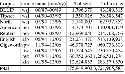
Corpus article name (mm/yy) # of sent. # of tokens BLLIP wsj 00/87–00/89 1,796,379 43,380,315 Tipster wsj 04/90–03/92 1,550,026 36,583,547 North wsj 07/94–12/96 2,748,803 62,937,557 American reu 04/94–07/96 4,773,701 110,001,109 Reuters reu 09/96–08/97 12,969,056 214,708,766 English afp 05/94–12/06 21,231,470 513,139,928 Gigaword apw 11/94–12/06 46,978,725 960,733,303 ltw 04/94–12/06 10,524,545 230,370,454 nyt 07/94–12/06 60,752,363 1,266,531,274 xin 01/95–12/06 12,624,835 283,579,330

total 175,949,903 3,721,965,583

Table 2: Details of the larger unlabeled data set used in English dependency parsing: sentences ex-ceeding 128 tokens in length were excluded for computational reasons.

as those described in (McDonald et al., 2005a; McDonald et al., 2005b; McDonald and Pereira, 2006; Koo et al., 2008). The English dependency-parsing data sets were constructed using a stan-dard set of head-selection rules (Yamada and Mat-sumoto, 2003) to convert the phrase structure syn-tax of the Treebank to dependency tree repre-sentations. We split the data into three parts: sections 02-21 for training, section 22 for de-velopment and section 23 for test. The Czech data sets were obtained from the predefined train-ing/development/test partition in the PDT. The un-labeled data for English was derived from the Brown Laboratory for Linguistic Information Pro-cessing (BLLIP) Corpus (LDC2000T43)2_{, giving}

a total of 1,796,379 sentences and 43,380,315 tokens. The raw text section of the PDT was used for Czech, giving 2,349,224 sentences and 39,336,570 tokens. These data sets are identical to the unlabeled data used in (Koo et al., 2008), and are disjoint from the training, development and test sets. The datasets used in our experiments are summarized in Table 1.

In addition, we will describe experiments that make use of much larger amounts of unlabeled data. Unfortunately, we have no data available other than PDT for Czech, this is done only for English dependency parsing. Table 2 shows the detail of the larger unlabeled data set used in our experiments, where we eliminated sentences that have more than 128 tokens for computational rea-sons. Note that the total size of the unlabeled data reaches 3.72G (billion) tokens, which is

mately 4,000 times larger than the size of labeled training data.

4.2 Features

4.2.1 Baseline Features

In general we will assume that the input sentences include both words and part-of-speech (POS) tags. Our baseline features (“baseline”) are very simi-lar to those described in (McDonald et al., 2005a; Koo et al., 2008): these features track word and POS bigrams, contextual features surrounding de-pendencies, distance features, and so on. En-glish POS tags were assigned by MXPOST (Rat-naparkhi, 1996), which was trained on the train-ing data described in Section 4.1. Czech POS tags were obtained by the following two steps: First, we used ‘feature-based tagger’ included with the PDT3_{, and then, we used the method described in}

(Collins et al., 1999) to convert the assigned rich POS tags into simplified POS tags.

4.2.2 Cluster-based Features

In a second set of experiments, we make use of the feature set used in the semi-supervised approach of (Koo et al., 2008). We will refer to this as the “cluster-based feature set” (CL). The BLLIP (43M tokens) and PDT (39M tokens) unlabeled data sets shown in Table 1 were used to construct the hierar-chical clusterings used within the approach. Note that when this feature set is used within the SS-SCM approach, the same set of unlabeled data is used to both induce the clusters, and to estimate the generative models within the SS-SCM model.

4.2.3 Constructing the Generative Models

As described in section 2.2, the generative mod-els in the SS-SCM approach are defined through a partition of the original feature vector f(x,y)

into k feature vectors r1(x,y). . .rk(x,y). We

follow a similar approach to that of (Suzuki and Isozaki, 2008) in partitioning f(x,y), where the

kdifferent feature vectors correspond to different feature types or feature templates. Note that, in general, we are not necessary to do as above, this is one systematic way of a feature design for this approach.

4.3 Other Experimental Settings

All results presented in our experiments are given in terms of parent-prediction accuracy on

unla-3_{Training, development, and test data in PDT already} con-tains POS tags assigned by the ‘feature-based tagger’.

beleddependency parsing. We ignore the parent-predictions of punctuation tokens for English, while we retain all the punctuation tokens for Czech. These settings match the evaluation setting in previous work such as (McDonald et al., 2005a; Koo et al., 2008).

We used the method proposed by (Carreras, 2007) for our second-order parsing model. Since this method only considers projective dependency structures, we “projectivized” the PDT training data in the same way as (Koo et al., 2008). We used a non-projective model, trained using an ap-plication of the matrix-tree theorem (Koo et al., 2007; Smith and Smith, 2007; McDonald and Satta, 2007) for the first-order Czech models, and projective parsers for all other models.

As shown in Section 2, SS-SCMs with 1st-order parsing models have two tunable parameters, C

and η, corresponding to the regularization con-stant, and the Dirichlet prior for the generative models. We selected a fixed valueη = 2, which was found to work well in preliminary experi-ments.4 _{The value ofC was chosen to optimize}

performance on development data. Note that C

for supervised SCMs were also tuned on develop-ment data. For the two-stage SS-SCM for incor-porating second-order parsing model, we have ad-ditional one tunable parameterB shown in Eq. 8. This was also chosen by the value that provided the best performance on development data.

In addition to providing results for models trained on the full training sets, we also performed experiments with smaller labeled training sets. These training sets were either created through random sampling or by using a predefined subset of document IDs from the labeled training data.

5 Results and Discussion

Table 3 gives results for the SS-SCM method un-der various configurations: for first and second-order parsing models, with and without the clus-ter features of (Koo et al., 2008), and for varying amounts of labeled data. The remainder of this section discusses these results in more detail.

5.1 Effects of the Quantity of Labeled Data

We can see from the results in Table 3 that our semi-supervised approach consistently gives gains

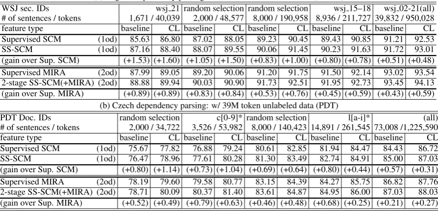
(a) English dependency parsing: w/ 43M token unlabeled data (BLLIP)

WSJ sec. IDs wsj 21 random selection random selection wsj 15–18 wsj 02-21(all) # of sentences / tokens 1,671 / 40,039 2,000 / 48,577 8,000 / 190,958 8,936 / 211,727 39,832 / 950,028 feature type baseline CL baseline CL baseline CL baseline CL baseline CL Supervised SCM (1od) 85.63 86.80 87.02 88.05 89.23 90.45 89.43 90.85 91.21 92.53 SS-SCM (1od) 87.16 88.40 88.07 89.55 90.06 91.45 90.23 91.63 91.72 93.01 (gain over Sup. SCM) (+1.53) (+1.60) (+1.05) (+1.50) (+0.83) (+1.00) (+0.80) (+0.78) (+0.51) (+0.48) Supervised MIRA (2od) 87.99 89.05 89.20 90.06 91.20 91.75 91.50 92.14 93.02 93.54 2-stage SS-SCM(+MIRA) (2od) 88.88 89.94 90.03 90.90 91.73 92.51 91.95 92.73 93.45 94.13 (gain over Sup. MIRA) (+0.89) (+0.89) (+0.83) (+0.84) (+0.53) (+0.76) (+0.45) (+0.59) (+0.43) (+0.59)

(b) Czech dependency parsing: w/ 39M token unlabeled data (PDT)

PDT Doc. IDs random selection c[0-9]* random selection l[a-i]* (all)

# of sentences / tokens 2,000 / 34,722 3,526 / 53,982 8,000 / 140,423 14,891 / 261,545 73,008 /1,225,590 feature type baseline CL baseline CL baseline CL baseline CL baseline CL Supervised SCM (1od) 75.67 77.82 76.88 79.24 80.61 82.85 81.94 84.47 84.43 86.72 SS-SCM (1od) 76.47 78.96 77.61 80.28 81.30 83.49 82.74 84.91 85.00 87.03 (gain over Sup. SCM) (+0.80) (+1.14) (+0.73) (+1.04) (+0.69) (+0.64) (+0.80) (+0.44) (+0.57) (+0.31) Supervised MIRA (2od) 78.19 79.60 79.58 80.77 83.15 84.39 84.27 85.75 86.82 87.76 2-stage SS-SCM(+MIRA) (2od) 78.71 80.09 80.37 81.40 83.61 84.87 84.95 86.00 87.03 88.03 (gain over Sup. MIRA) (+0.52) (+0.49) (+0.79) (+0.63) (+0.46) (+0.48) (+0.68) (+0.25) (+0.21) (+0.27)

Table 3: Dependency parsing results for the SS-SCM method with different amounts of labeled training data. Supervised SCM (1od) and Supervised MIRA (2od) are the baseline first and second-order ap-proaches; SS-SCM (1od) and 2-stage SS-SCM(+MIRA) (2od) are the first and second-order approaches described in this paper. “Baseline” refers to models without cluster-based features, “CL” refers to models which make use of cluster-based features.

in performance under various sizes of labeled data. Note that the baseline methods that we have used in these experiments are strong baselines. It is clear that the gains from our method are larger for smaller labeled data sizes, a tendency that was also observed in (Koo et al., 2008).

5.2 Impact of Combining SS-SCM with Cluster Features

One important observation from the results in Ta-ble 3 is that SS-SCMs can successfully improve the performance over a baseline method that uses the cluster-based feature set (CL). This is in spite of the fact that the generative models within the SS-SCM approach were trained on the same un-labeled data used to induce the cluster-based fea-tures.

5.3 Impact of the Two-stage Approach

Table 3 also shows the effectiveness of the two-stage approach (described in Section 3.2) that inte-grates the SS-SCM method within a second-order parser. This suggests that the SS-SCM method can be effective in providing features (generative models) used within a separate learning algorithm, providing that this algorithm can make use of real-valued features.

91.5 92.0 92.5 93.0 93.5

10 100 1,000 10,000

CL

baseline

43.4M 143M

468M 1.38G 3.72G

(Mega tokens) Unlabeled data size: [Log-scale]

P

a

r

e

n

t

-p

r

e

d

i

c

t

i

o

n

A

c

c

u

r

a

c

y

(BLLIP)

Figure 1: Impact of unlabeled data size for the SS-SCM on development data of English dependency parsing.

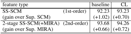
5.4 Impact of the Amount of Unlabeled Data

unla-feature type baseline CL

SS-SCM (1st-order) 92.23 93.23

(gain over Sup. SCM) (+1.02) (+0.70) 2-stage SS-SCM(+MIRA) (2nd-order) 93.68 94.26 (gain over Sup. MIRA) (+0.66) (+0.72)

Table 4: Parent-prediction accuracies on develop-ment data with 3.72G tokens unlabeled data for English dependency parsing.

beled data. Note, however, that the gain in perfor-mance as unlabeled data is added is not as sharp as might be hoped, with a relatively modest dif-ference in performance for 43.4 million tokens vs. 3.72 billion tokens of unlabeled data.

5.5 Computational Efficiency

The main computational challenge in our ap-proach is the estimation of the generative mod-els q = hq1. . . qki from unlabeled data,

partic-ularly when the amount of unlabeled data used is large. In our implementation, on the 43M to-ken BLLIP corpus, using baseline features, it takes about 5 hours to compute the expected counts re-quired to estimate the parameters of the generative models on a single 2.93GHz Xeon processor. It takes roughly 18 days of computation to estimate the generative models from the larger (3.72 billion word) corpus. Fortunately it is simple to paral-lelize this step; our method takes a few hours on the larger data set when parallelized across around 300 separate processes.

Note that once the generative models have been estimated, decoding with the model, or traing the model on labeled data, is relatively in-expensive, essentially taking the same amount of computation as standard dependency-parsing ap-proaches.

5.6 Results on Test Data

Finally, Table 5 displays the final results on test data. There results are obtained using the best setting in terms of the development data perfor-mance. Note that the English dependency pars-ing results shown in the table were achieved us-ing 3.72 billion tokens of unlabeled data. The im-provements on test data are similar to those ob-served on the development data. To determine statistical significance, we tested the difference of parent-prediction error-rates at the sentence level using a paired Wilcoxon signed rank test. All eight comparisons shown in Table 5 are significant with

(a) English dependency parsing: w/ 3.72G token ULD

feature set baseline CL

SS-SCM (1st-order) 91.89 92.70

(gain over Sup. SCM) (+0.92) (+0.58) 2-stage SS-SCM(+MIRA) (2nd-order) 93.41 93.79 (gain over Sup. MIRA) (+0.65) (+0.48) (b) Czech dependency parsing: w/ 39M token ULD (PDT)

feature set baseline CL

SS-SCM (1st-order) 84.98 87.14

(gain over Sup. SCM) (+0.58) (+0.39) 2-stage SS-SCM(+MIRA) (2nd-order) 86.90 88.05 (gain over Sup. MIRA) (+0.15) (+0.36)

Table 5: Parent-prediction accuracies on test data using the best setting in terms of development data performances in each condition.

(a) English dependency parsers on PTB dependency parser test description (McDonald et al., 2005a) 90.9 1od (McDonald and Pereira, 2006) 91.5 2od

(Koo et al., 2008) 92.23 1od, 43M ULD SS-SCM (w/ CL) 92.701od, 3.72G ULD (Koo et al., 2008) 93.16 2od, 43M ULD 2-stage SS-SCM(+MIRA, w/ CL) 93.792od, 3.72G ULD

(b) Czech dependency parsers on PDT dependency parser test description (McDonald et al., 2005b) 84.4 1od (McDonald and Pereira, 2006) 85.2 2od

(Koo et al., 2008) 86.07 1od, 39M ULD (Koo et al., 2008) 87.13 2od, 39M ULD SS-SCM (w/ CL) 87.141od, 39M ULD 2-stage SS-SCM(+MIRA, w/ CL) 88.052od, 39M ULD

Table 6: Comparisons with the previous top sys-tems: (1od, 2od: 1st- and 2nd-order parsing model, ULD: unlabeled data).

p <0.01.

6 Comparison with Previous Methods

Table 6 shows the performance of a number of state-of-the-art approaches on the English and Czech data sets. For both languages our ap-proach gives the best reported figures on these datasets. Our results yield relative error reduc-tions of roughly 27% (English) and 20% (Czech) over McDonald and Pereira (2006)’s second-order supervised dependency parsers, and roughly 9% (English) and 7% (Czech) over the previous best results provided by Koo et. al. (2008)’s second-order semi-supervised dependency parsers.

2005). In particular, both methods use a two-stage approach; They first train generative models or auxiliary problems from unlabeled data, and then, they incorporate these trained models into a super-vised learning algorithm as real valued features. Moreover, both methods make direct use of exist-ing feature-vector definitions f(x,y) in inducing representations from unlabeled data.

7 Conclusion

This paper has described an extension of the semi-supervised learning approach of (Suzuki and Isozaki, 2008) to the dependency parsing problem. In addition, we have described extensions that in-corporate the cluster-based features of Koo et al. (2008), and that allow the use of second-order parsing models. We have described experiments that show that the approach gives significant im-provements over state-of-the-art methods for de-pendency parsing; performance improves when the amount of unlabeled data is increased from 43.8 million tokens to 3.72 billion tokens. The ap-proach should be relatively easily applied to lan-guages other than English or Czech.

We stress that the SS-SCM approach requires relatively little hand-engineering: it makes di-rect use of the existing feature-vector representa-tion f(x,y) used in a discriminative model, and does not require the design of new features. The main choice in the approach is the partitioning off(x,y) into componentsr1(x,y). . .rk(x,y),

which in our experience is straightforward.

References

R. Kubota Ando and T. Zhang. 2005. A Framework for Learning Predictive Structures from Multiple Tasks and Unlabeled Data. Journal of Machine Learning Research, 6:1817–1853.

J. K. Baker. 1979. Trainable Grammars for Speech Recognition. InSpeech Communication Papers for the 97th Meeting of the Acoustical Society of Amer-ica, pages 547–550.

J. Blitzer, R. McDonald, and F. Pereira. 2006. Domain Adaptation with Structural Correspondence Learn-ing. InProc. of EMNLP-2006, pages 120–128. P. F. Brown, P. V. deSouza, R. L. Mercer, V. J. Della

Pietra, and J. C. Lai. 1992. Class-based n-gram Models of Natural Language. Computational Lin-guistics, 18(4):467–479.

S. Buchholz and E. Marsi. 2006. CoNLL-X Shared Task on Multilingual Dependency Parsing. InProc. of CoNLL-X, pages 149–164.

X. Carreras. 2007. Experiments with a Higher-Order Projective Dependency Parser. InProc. of EMNLP-CoNLL, pages 957–961.

M. Collins, J. Hajic, L. Ramshaw, and C. Tillmann. 1999. A Statistical Parser for Czech. In Proc. of ACL, pages 505–512.

J. Eisner. 1996. Three New Probabilistic Models for Dependency Parsing: An Exploration. In Proc. of COLING-96, pages 340–345.

Jan Hajiˇc. 1998. Building a Syntactically Annotated Corpus: The Prague Dependency Treebank. In Is-sues of Valency and Meaning. Studies in Honor of Jarmila Panevov´a, pages 12–19. Prague Karolinum, Charles University Press.

T. Koo, A. Globerson, X. Carreras, and M. Collins. 2007. Structured Prediction Models via the Matrix-Tree Theorem. In Proc. of EMNLP-CoNLL, pages 141–150.

T. Koo, X. Carreras, and M. Collins. 2008. Simple Semi-supervised Dependency Parsing. In Proc. of ACL-08: HLT, pages 595–603.

J. Lafferty, A. McCallum, and F. Pereira. 2001. Condi-tional Random Fields: Probabilistic Models for Seg-menting and Labeling Sequence Data. In Proc. of ICML-2001, pages 282–289.

D. C. Liu and J. Nocedal. 1989. On the Limited Memory BFGS Method for Large Scale Optimiza-tion. Math. Programming, Ser. B, 45(3):503–528. M. P. Marcus, B. Santorini, and M. A. Marcinkiewicz.

1994. Building a Large Annotated Corpus of En-glish: The Penn Treebank. Computational Linguis-tics, 19(2):313–330.

R. McDonald and F. Pereira. 2006. Online Learning of Approximate Dependency Parsing Algorithms. In Proc. of EACL, pages 81–88.

R. McDonald and G. Satta. 2007. On the Com-plexity of Non-Projective Data-Driven Dependency Parsing. InProc. of IWPT, pages 121–132.

R. McDonald, K. Crammer, and F. Pereira. 2005a. On-line Large-margin Training of Dependency Parsers. InProc. of ACL, pages 91–98.

R. McDonald, F. Pereira, K. Ribarov, and J. Hajiˇc. 2005b. Non-projective Dependency Parsing us-ing Spannus-ing Tree Algorithms. In Proc. of HLT-EMNLP, pages 523–530.

J. Nivre, J. Hall, S. K¨ubler, R. McDonald, J. Nilsson, S. Riedel, and D. Yuret. 2007. The CoNLL 2007 Shared Task on Dependency Parsing. In Proc. of EMNLP-CoNLL, pages 915–932.

A. Ratnaparkhi. 1996. A Maximum Entropy Model for Part-of-Speech Tagging. In Proc. of EMNLP, pages 133–142.

D. A. Smith and J. Eisner. 2007. Bootstrapping Feature-Rich Dependency Parsers with Entropic Pri-ors. InProc. of EMNLP-CoNLL, pages 667–677. D. A. Smith and N. A. Smith. 2007.

Probabilis-tic Models of Nonprojective Dependency Trees. In Proc. of EMNLP-CoNLL, pages 132–140.

J. Suzuki and H. Isozaki. 2008. Semi-supervised Sequential Labeling and Segmentation Using Giga-Word Scale Unlabeled Data. InProc. of ACL-08: HLT, pages 665–673.

Q. I. Wang, D. Schuurmans, and D. Lin. 2008. Semi-supervised Convex Training for Dependency Pars-ing. InProc. of ACL-08: HLT, pages 532–540. H. Yamada and Y. Matsumoto. 2003. Statistical